Article

A Satellite-Based Tool for Mapping Evaporation in Inland Water Bodies: Formulation, Application, and Operational Aspects

Institute for Electromagnetic Sensing of the Environment (IREA), National Research Council of Italy (CNR), Via Corti, 12-20133 Milano, Italy
*
Author to whom correspondence should be addressed.
These authors contributed equally to this work.
Remote Sens. 2022, 14(11), 2636; https://doi.org/10.3390/rs14112636
Submission received: 29 April 2022 / Revised: 23 May 2022 / Accepted: 30 May 2022 / Published: 31 May 2022
(This article belongs to the Topic Remote Sensing in Water Resources Management Models)

Abstract

:
With the increase of evaporation projected for water bodies worldwide, there is a growing need for flexible and low data-demanding tools enabling the monitoring and management of water resources. This study presents a simple satellite-based tool named LakeVap specifically designed for mapping evaporation from lakes and reservoirs. LakeVap requires a small amount of potentially available data with a global coverage. The tool follows a Dalton-type approach and produces instantaneous (i.e., hourly) and daily evaporation maps from satellite-derived Lake Surface Water Temperature (LSWT) maps and single-point/gridded meteorological data. The model is tested on Lake Garda, Italy, by using a long time series of LSWT (ESA CCI-Lakes) and different sources of meteorological forcing. The accuracy of LakeVap evaporation outputs is checked by comparison with those from a hydro-thermodynamic model (Delft3D) specifically set up and validated for the case study. Results are consistent and sensitive to the representativeness of the meteorological forcing. In the test site, wind speed is found to be the most spatially variable parameter, and it is significantly underestimated by the ERA5 meteorological dataset (up to 100%). The potential application of LakeVap to other case studies and in operational contexts is discussed.

Graphical Abstract

1. Introduction

At all latitudes and climates, evaporation from water surfaces is a key component of the overall budget of heat and water volume in natural and artificial reservoirs. Under the perspective of global warming, drying climate, and water scarcity, several studies have projected a general increase in lake evaporation [1,2] due to the alteration of environmental drivers sensitive to climate change such as air and water temperature, air vapor content, wind speed, and solar radiation [3]. How and to what extent evaporation from lakes increases differs worldwide [4], as the hydroclimatic variables involved in this process depend on the climatic region [5] and the lake’s thermal behavior [6]. Many investigations available in the literature address this issue in arid and semi-arid contexts, where lakes suffer from water deficit when evaporation exceeds precipitation, thus implying in some cases significant groundwater uptake to compensate for the water balance (e.g., [7]). However, lake evaporation is an issue in temperate to boreal environments as well. In these regions, evaporation is strongly correlated with the duration of the ice-cover period, whose climate-induced reduction is leading to a general increase of evaporation losses for many lakes of this kind (e.g., Lake Superior [8], White Bear Lake [9]). Similarly, at high altitudes (e.g., in the Tibetan Plateau), lake evaporation tightly interacts with increasing trends of precipitation and glacier melting and contributes to the expansion of new lakes [10,11].
Several methods have been proposed over the years to estimate evaporation from inland waters. A summary of the most known and used evaporation models and their characteristics is presented in Table 1. In the table, evaporation models are grouped into five categories following a commonly used distinction [12,13]: simplified, mass balance, energy budget, mass transfer, and combined models. Such methods differ by the underlying physical assumptions, complexity, and amount of input variables required and most often have associated practical challenges and large uncertainties [14]. Countless comparative studies exist whose only aim is to test which method is better for estimating evaporation from specific case studies from dry to continental and humid climatic areas [12,15,16,17,18]. The simplified methods demand less data, but they require a significant effort in the calibration of the empirical coefficients relating evaporation to, e.g., solar radiation/daylight hours and air temperature. However, when well-tuned, these methods can provide routine evaporation measures, as in the case of Mirror Lake in the USA [16]. Among the energy budget methods, the simplified Bowen Ratio Energy Balance (BREB) is the most used in aquatic environments and is often taken as a reference in the comparison of models [13,17,19]. The conclusion of most comparative studies is generally that the best results are obtained with combination models because they consider both the aerodynamic term (and thus the effect of wind in enhancing the heat transfer from water to air) and the energy stored by the water body, which determines a phase lag between net radiation and evaporation, especially in deep lakes. Needless to say, these methods are also the most data-demanding and the least used by water managers, who most often rely on evaporation pan measurements [20].
One additional complication to the estimation of evaporation from lakes and water reservoirs, in general, is the number of monitoring points, especially in large and medium-sized lakes. Spatial patterns of evaporation indeed exist not only among different hydroclimatic areas [4] but also inside single lakes. Most studies dealing with evaporation (and more generally with heat exchanges between lakes and atmosphere) rely on one-point measurements and/or estimations, while significant spatial gradients have been found in the surface net heat flux [21,22], leading to spatial patterns of latent heat flux and evaporation rates [23,24]. Traditional field approaches cannot satisfy the need to understand the spatial heterogeneity of these fluxes. To overcome this limitation, RS-based models [25,26,27,28] can be used to benefit from the synoptic properties of satellite measurements. In particular, SEBAL [25], METRIC [27], and SEBS [28] are RS-energy based models and are developed to retrieve actual evapotranspiration from land surfaces (e.g., at watershed level). Hence, these methods are not purposely built for water surfaces, and their use for estimating evaporation rates from water bodies is not always robust. For instance, the SEBAL model [25] treats water surfaces as boundary conditions ,where the so-called “cold pixel” is set, evaporation is supposed to be at its maximum value, and sensible heat flux is supposed to be zero. In addition, these models make very general assumptions on the formulation of the heat exchanges between air and the water body: e.g., in a METRIC application in the USA [29], the authors assume that the net heat flux between the atmosphere and the water body is approximately 50% of net radiation at the water surface; the authors of [30] assume that there is, instead, a linear dependence depending on the time of the year. Such general assumptions do not hold for all lakes, whose evaporation dynamics depend on many factors, not least the heat storage capacity and the thermal regime of the water body. In some cases, however, promising correlations are found between such RS-energy based models and more conventional methods, such as those listed in Table 1 (see, e.g., [31] for Lake Nasser in Egypt and [32] for Amirkabir dam in Iran). Efforts towards the inclusion of the thermal capacity of both fresh and saline water bodies are found in, e.g., [33,34]. The latter integrates satellite-derived data (e.g., surface water extent) and physical modeling (based on the energy budget) for five American reservoirs and find very good agreement between modeled and measured evaporation rates. Interestingly, the authors do not use satellite-derived Lake Surface Water Temperature (LSWT) in their model, but they acknowledge that including such information in the calculation can improve the accuracy of evaporation estimates.
The advantages of an RS-based approach are not limited to the possibility of retrieving the spatial distribution of the evaporation rates. The increasing availability of datasets integrating multiple sensor products and thousands of lakes and reservoirs around the globe represents a valuable opportunity for investigating long-term trends of evaporation at both local and global scales [34]. At the same time, there is a need for flexible and appropriate tools, requiring as little data as possible, to enable the monitoring and management of the water resources.
In this contribution, we present a satellite-based tool named LakeVap for estimating evaporation rates from lakes. LakeVap aims at meeting the above-mentioned requisites of long temporal and fine spatial coverage as well as flexibility, handiness, and little data demand. The tool combines the spatially resolved information of Lake Surface Water Temperature (LSWT) contained in satellite-derived maps with single-point or gridded meteorological data from in-situ stations or atmospheric/land models. LakeVap estimates the instantaneous evaporation from the water surface following a Dalton-type approach (see Table 1) and applies an energy budget scheme for deriving daily evaporation. LakeVap is here showcased for Lake Garda, a well-studied sub-alpine lake, where a consistent and long-term dataset of remote sensing products, meteorological in-situ measurements, and model data is available. Since direct measurements of evaporation are not available at the test site, we compare the estimates of our LakeVap with the results of a coupled atmospheric and thermo-hydrodynamic model both purposely calibrated for the test site and validated for the period 2004–2018 (WRF, Weather Research and Forecasting model + Delft3D, [35]). LakeVap is here tested with LSWT maps available for Lake Garda from the dataset created under the ESA Climate Change Initiative for Lakes (CCI-Lakes) and with multiple meteorological datasets, ranging from in-situ observations to local and global atmospheric/land models.
Table 1. Summary of the main characteristics of most commonly used evaporation models.
ModelNameMethodologyInput VariablesStrengthsConstrainsReferences
SimplifiedStephens–Stewart
Makkink, Doorenbos–Pruitt, Jensen–Haise
Empirical relations between evaporation and solar radiationAir temperature, solar radiationVery low data demand
If properly tuned, they can provide cost-effective evaporation estimates
Site-specific, they require some empirical coefficients to be calibrated[36,37,38,39]
Blaney–Criddle,Empirical relations between evaporation and daylight hoursAir temperature, daylight hours[16,36,40]
Papadakis, Thornthwaite
Mass balance Calculates the water budget of the water bodyInflows, rainfall, runoff, outflows, water levelsVery accurate if the water budget is properly closedExtremely data demanding
Require continuous and accurate measurements of the input variables
e.g., [41]
Energy budgetBREB
RS-based (SEBAL, METRIC, SEBS, AquaSEBS)
Calculate all the energy contributions entering and exiting the water bodySolar radiation, water temperature, air temperature, wind speed, relative humidityProvide a comprehensive description of the energy balance.
If RS-based, they provide evaporation maps
Data demanding[13,17,31,42]
[25,27,28,33]
Mass transfer or bulk transfer Dalton’s law (Dalton 1802)Water temperature, air temperature, wind speed, relative humidityLow data demandRequires the tuning of the wind functione.g., [43]
CombinedPriestly–Taylor,
de Bruin,
Brutsaert and Sticker,
Penman
Combine radiative and aerodynamic termsAll variables required by the energy budget and mass transfer modelsMost accurate
Consider the energy stored by the water body
Most data demanding[44,45,46,47,48]
In the following pages, we first present a detailed description of the model behind LakeVap and its equations (Section 2.1); then, we show the study site (Lake Garda, Section 2.2) and the datasets used (Section 2.3). In the results, we show the potential of LakeVap to produce a long time series of instantaneous evaporation maps (Section 3.1). The quality of the results of LakeVap is tested by comparison with the evaporation outputs of the reference Delft3D hydrodynamic model (Section 3.2). In Section 3.3, we investigate how our LakeVap instantaneous evaporation estimates vary when using different meteorological sources, while considerations on the spatial variability of instantaneous evaporation maps are provided in Section 3.4. In the Discussion (Section 4), we comment on the LakeVap tool’s performance and give an overview of its functionalities.

2. Materials and Methods

2.1. The LakeVap Tool

LakeVap is a low data-demanding tool producing instantaneous and daily evaporation maps from water bodies. It can be applied to any inland water surface whose surface temperature is provided by satellite thermal sensors and can be routinely applied following the satellite revisiting time period. Since it is based on satellite-derived thermal products, it is constrained by clear sky conditions at the satellite overpass time and by the spatial resolution of the sensor used to measure LSWT.

2.1.1. Formulation

The LakeVap tool computes instantaneous evaporation rates from water surfaces by following the Dalton’s law (mass transfer theory) as proposed by [49]:
λ E = f   ( e w e a )
where E is the hourly evaporation rate ( mm / h ), λ   = 2444 kJ / kg is the water latent heat of vaporization, ( e w e a ) is the vapor pressure gradient between air at the air–water interface and air at 2 m a.w.l., and f is an empirical wind function specific for the study site. In the LakeVap tool, the wind function is defined following [49] (from [50]):
f = 4.8 + 1.98 u + 0.28 ( T w T a )
where T w is the water temperature derived from LSWT maps and T a is air temperature from observations or atmospheric models. Hence, in our tool, evaporation is proportional to the vapor pressure gradient, to wind speed, and to the thermal difference between water and air. We refer to the Supplementary Material S1 for the computation of the vapor pressure terms. From now on, we refer to instantaneous evaporation E h as the evaporation rate in mm / h obtained by computing E from Equation (1) based on the atmospheric conditions (i.e., air temperature and humidity, wind velocity) and on the surface temperature of the water body at a specific time of the day, coinciding with the satellite overpass.
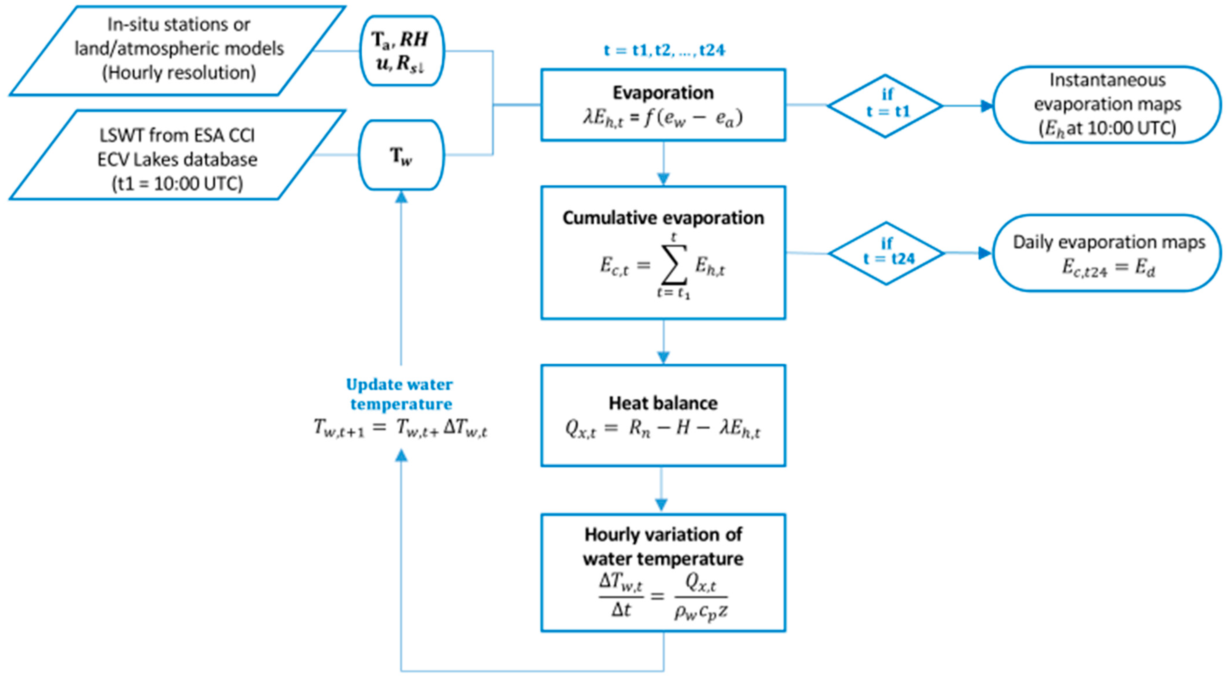
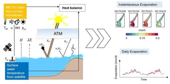
In addition to the instantaneous evaporation rate from Equation (1), LakeVap computes the daily evaporation by implementing a simple heat balance equation, which computes the energy stored in the water body based on all contributions of entering and exiting thermal energy (Figure 1).
The energy stored in the water body ( Q x ) is the result of a balance between a radiative term ( R n ), an advective term ( Q v ), and three negative contributions from the fluxes of sensible energy ( H ), latent energy (λ E ), and the energy exchanged with the bottom ( G ). The net radiative term R n represents the residual from the radiative balance at the water–air interface in terms of short ( R s ) and long ( R l ) wave radiation, considering the incident (i.e., directly coming from the sun, transmitted by the atmosphere, and diffused by the atmosphere), the reflected, and the emitted energy from the water body (depending on the water temperature). The advective term Q v is the net thermodynamic energy flux accounting for the contributions from surface and underground inflows/outflows ( F i n / F o u t ) and from precipitation ( F p ). The sensible energy H is the energy exchanged between the water surface and the air due to temperature differences, while the latent energy λ E is the energy exchanged during the evaporation process.
In LakeVap, we consider the advective energy Q v and the exchanges with the bottom G to be small compared to the other terms contributing to the net energy stored in the water body. This condition applies to many cases (e.g., [51]). Hence, the energy balance equation in LakeVap is simplified to Equation (3):
Q x = R n H λ E
where R n is the net radiation at the surface of the water body, H is the sensible energy, and λ E is the latent energy computed as in Equation (1). We refer to the Supplementary Material S1 for the full description of the heat balance terms.
The heat balance is computed at the time of the satellite overpass (10:00 a.m. UTC), based on the instantaneous values of each term, such that the energy stored by the water body Q x is obtained. The quantity Q x is then used to determine the changes in LSWT in the next hour following Equation (4):
Δ T w , t Δ t = Q x , t ρ w c p z
where Δ T w , t is the variation in water temperature at time t , Δ t is the variation in time (set as 1 h), Q x , t is the energy stored by the water body at time t , ρ w is the density of water ( 1000   kg   m 3 ), c p is the specific heat of water ( 4180   J   kg 1   K 1 ), and z is the thickness of the water storing the energy Q x , t . Here it is set to 1 m after some testing.
At the next time step (i.e., the subsequent hour), a new map of LSWT is produced by summing
T w , t + 1 = T w , t + Δ T w , t
Based on the updated LSWT map and the meteorological data for the new time step, all the terms of the heat balance (including evaporation) are computed again in a loop for the subsequent 23 h.
E d   = t = t 1 t = t 1 + 23 E h   ( t )
In this way, the daily evaporation E d is obtained as the cumulative sum of the hourly evaporation over 24 h.

2.1.2. Inputs and Outputs of the Model

Following the equations reported in Section 2.1.1 and Supplementary Material S1, the inputs of the LakeVap tool are the following:
  • Water temperature T w , from now on referred to as Lake Surface Water Temperature (LSWT) from EO data at the satellite overpass time (i.e., between 9:30 and 10:30 UTC in the CCI-Lakes dataset). We took 10:00 UTC as a reference time;
  • Downward shortwave radiation R s ;
  • Air temperature T a ;
  • Wind speed u ;
  • Relative humidity R H .
Atmospheric inputs 2–5 must be provided at an hourly resolution covering the 24 h from the satellite overpass in case of daily evaporation computation (e.g., from 10:00 UTC to 09:00 UTC of the following day based on the CCI-Lakes dataset reference time). The sources of these inputs can be in-situ meteorological stations or global models such as GLDAS (Global Land Data Assimilation System dataset from National Aeronautics and Space Administration (NASA): https://ldas.gsfc.nasa.gov/gldas, accessed on 3 February 2021) and ERA5 (ECMWF Reanalysis v5 from the European Centre for Medium-Range Weather Forecast: https://www.ecmwf.int/en/forecasts/datasets/reanalysis-datasets/era5, accessed on 9 February 2021), as well as numerical weather models specifically set up for the study area, e.g., WRF (Weather Research and Forecasting model by the National Center for Atmospheric Research (NCAR): https://www.mmm.ucar.edu/weather-research-and-forecasting-model, accessed on 28 April 2022) or COSMO (by Consortium for Small-Scale Modeling: http://www.cosmo-model.org, accessed on 28 April 2022). Due to the potentially different sources of these variables, the LakeVap tool accepts different formats: time series of single values (e.g., when coming from a single weather station or a spatial average of model grid points) or gridded fields (e.g., from spatially resolved model data).
We recall that the LakeVap tool is designed to provide two different outputs:
  • Maps of instantaneous evaporation ( E h ) at satellite overpass;
  • Maps of daily evaporation ( E d ) estimated during the 24 h including and after the satellite overpass (e.g., from 10:00 UTC to 09:00 UTC of the following day based on the CCI-Lakes dataset reference time). Daily evaporation is obtained by summing the hourly values estimated over the 24 h from the satellite overpass time.
The procedure for the evaporation rate mapping is summarized in Figure 2.

2.2. Study Site

We test the LakeVap tool in Lake Garda, Italy, where an extensive dataset from in-situ measurements, remote sensing imagery, and numerical modeling is available.
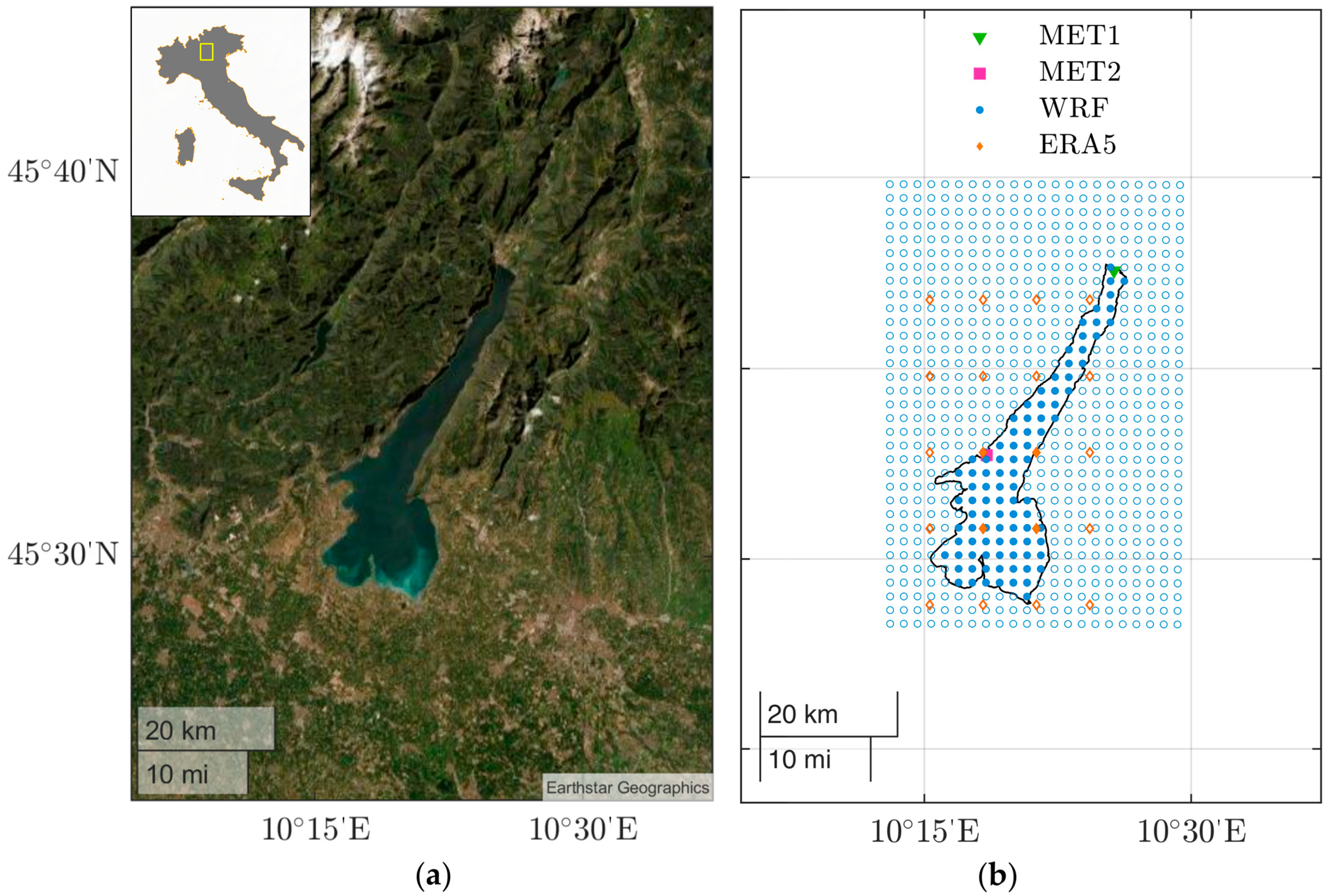
Lake Garda is one of the most important subalpine lakes in Europe and the largest in Italy. It is located in the northern part of Italy, with a lake surface area of 368 km2, a maximum length of 52 km along its main axis, and a maximum width of 18 km in the southern part of the lake, with a total perimeter of 162 km. The shape of the lake (Figure 3a) combines a large and relatively simple round-shaped geometry in the southern part with an elongated and narrow area surrounded by a steep orography in the northern trunk directed along a NE–SW axis.
Due to the specific shape of the lake and topography of the region, Lake Garda is subject to local breezes with specific timing and spatial patterns. In the northern part of the lake, winds are stronger since they are channeled by the steep lateral mountains and blow along the lake’s longitudinal axis. Summer breezes in this area have alternating provenance [52] based on the thermal gradients between the lake and the terrain in the northern valleys. In the southern basin, several local breezes blow in diverse directions, with lower intensity and duration. Thus, the spatial distribution of the wind field is typically heterogeneous in Lake Garda, except for some strong synoptic events in which an almost uniform strong wind moves the lake surface.
Such heterogeneity also affects the thermal behavior of the lake. The thermal regime of Lake Garda is classified as oligomictic [53,54], which means that the lake experiences complete overturns only in some years when cold winter air temperature and strong wind events allow the water column to fully mix. However, additional factors influencing the mixing regime of this lake were found to be wind-driven deep ventilation, the Earth’s rotation [55], and the interaction between the two sub-basins [56].
Oligomixis only applies to the northern deep sub-basin, while the southern sub-basin is subject to complete mixing every year due to the shallower bathymetry [35]. In general, the different behavior of the two sub-basins results from the different ways they exchange heat through the water surface, which is a direct consequence of the different morphological characteristics as well as different atmospheric forcing. This also causes a typical surface temperature gradient, with the southern part of the lake being warmer than the northern part, which is visible from either in-situ data or remote sensing imagery [35,57,58].

2.3. Data

For the computation of instantaneous and daily evaporation rate estimation, LakeVap requires LSWT imagery from satellites and atmospheric data, as anticipated in Section 2.1.2. In the following sections, we detail the source of the data used and the reasons behind the choice. Table 2 summarizes the key information on the data used, including the temporal availability of data and the data provider.

2.3.1. Remote Sensing Imagery from CCI-Lakes Database

A comprehensive dataset of satellite imagery of Lake Garda from optical and thermal sensors exists (e.g., [60]). To test the LakeVap tool, we used LSWT maps derived from thermal bands of different sensors (e.g., MODIS, AVHRR) from the ESA CCI ECV Lakes dataset (https://climate.esa.int/en/odp, accessed on 17 May 2021) (from now on, CCI-Lakes). This dataset provided 1923 LSWT maps of Lake Garda at 1 km resolution from 1995 to 2019 with a standardized format and quality information. More than 50% of the images are available at a 1–2 day time resolution, with the largest gaps registered in the period preceding 2002. For this work, we selected those maps having more than 55% of pixels with quality level 4 or 5 [61], for a total number of 1196 images.

2.3.2. Meteorological Data

Meteorological data in Lake Garda are available in either in-situ measurements or atmospheric/land models.
As for in-situ data, regular measurements of the main atmospheric variables are taken at several ground weather stations operated by various local environmental protection agencies (see [35] for a complete overview of active stations). In this work, we used data from the northernmost station of Riva del Garda and Toscolano Maderno, located at the end of the northern trunk (respectively, MET1 and MET2 in Figure 3b). MET1 was chosen as this station provides the longest time series (from 1990 to date) covering the entire period of availability of CCI-Lakes LSWT maps; the station is managed by the Edmund Mach Foundation (FEM -Data can be obtained under formal request). MET2 data were also included as [35] showed that it was the best-represented weather station by the WRF model in terms of wind speed over the lake; the station is managed by the Environmental Protection Agency of the Lombardy Region (ARPA Lombardia). We used measurements at hourly resolution of the following variables: air temperature (°C) at 2 m a.g.l.; relative humidity (%) 2 m a.g.l.; solar radiation (MJ/m2) (from MET1 only, converted to W/m2); wind velocity (m/s) at 10 m a.g.l. Wind speed is measured at 5 m a.g.l. in MET1; hence, this measurement was rescaled at 10 m a.g.l. assuming a logarithmic profile for a neutrally stratified atmosphere and a roughness length of 0.001 m, as the station is located on a dock.
As for model data, we used ERA5-Land hourly data from ECMWF climate reanalysis [62] and Weather Research and Forecasting (WRF [63]) model outputs over the Lake Garda Region ([35,59]).
ERA5-Land is a reanalysis dataset providing land variables produced by replaying the land component of the ECMWF ERA5 climate reanalysis at a finer resolution than ERA5 Climate reanalysis. Data can be freely downloaded for the entire globe from Copernicus Open Access Hub (https://cds.climate.copernicus.eu/cdsapp#!/dataset/reanalysis-era5-land?tab=overview, accessed on 9 February 2021) and are available from 1950 to the present at the horizontal resolution of 0.1° × 0.1° (~11 km) and at the time resolution of 1 h. From this dataset, we downloaded the following weather variables at the numerical grid points covering Lake Garda: air temperature (K) at 2 m a.g.l.; dew point temperature (K) at 2 m a.g.l. converted to relative humidity (%) based on air temperature [64]; downward short-wave radiation (J/m2), converted to W/m2, U-component (east–west) of wind velocity (m/s) at 10 m a.g.l.; V-component (south–north) of wind velocity (m/s) at 10 m a.g.l. Wind velocity was obtained from the U and V component as W = U 2 + V 2 . From now on, we refer to ERA5-Land as ERA5 for brevity. Among the grid points lying within the Lake Garda area, in-lake points were selected (filled magenta circles Figure 3b) and a spatial average was performed to have one value representing the mean weather conditions over the lake.
The Weather Research and Forecasting (WRF) model was run ad-hoc over the Lake Garda region by [59] and extended in [35] for a long run from 2004 to 2018. The model provides time and space-varying fields at the horizontal resolution of 2 km and time resolution of 1 h of the following variables: air temperature (K) at 2 m a.g.l.; relative humidity (%) at 2 m a.g.l., downward short-wave radiation flux (W/m2), U-component (east–west) of wind velocity (m/s) at 10 m a.g.l.; V-component (south–north) of wind velocity (m/s) at 10 m a.g.l. Wind velocity was obtained from the U and V component as shown before for ERA5 data. From now on, we refer to data derived from the WRF model as WRF for brevity. As for the ERA5 dataset, atmospheric variables from in-lake WRF points were selected (see Figure 3b) and spatially averaged. Given the higher spatial resolution of the WRF dataset, additional tests of the LakeVap tool were performed by feeding the model with fields of atmospheric variables simulated by the WRF model. These tests are better described in Section 2.4, while the results are discussed in Section 3.4.

2.3.3. Delft3D Hydro-Thermodynamic Model

To evaluate the performances of the LakeVap tool in estimating the evaporation rates, we use the model results of a 3D hydro-thermodynamic model (Delft3D by Deltares [65]) specifically set up for the test site. A Delft3D-FLOW model was previously calibrated and validated by [35] for Lake Garda and already used for several modeling and RS applications (e.g., [35,56,66]). The availability of this model’s results coincides with that of the WRF outputs mentioned above, as the Delft3D model is one-way coupled with the WRF long run from 2004 to 2018. The model simulates the three-dimensional temperature, flow, and turbulence field in Lake Garda. Each term of the heat balance equation is computed in each horizontal grid cell and considers the weather forcing coming from the WRF model and the water temperature of the surface layer, which in turn is affected by the three-dimensional flow field simulated in the lake. Evaporative flux is computed as part of the heat balance between the lake and the above atmosphere following a Dalton law of the kind
λ E = ϱ a c e   ( q s q a )
where ϱ a is the density of air, c e is a constant calibrated for Lake Garda, and q s , q a are the specific humidity of saturated air (at the water level) and air, respectively, at 10 m above water level. For more details on the numerical values of the calibration constant and on the equations implemented in Delft3D-Flow, we refer to [35] and to the Delft3D-Flow manual.

2.4. LakeVap Tool Runs and Evaluation Metrics

In Section 3, results from different LakeVap tool runs are presented.
The first four model runs are aimed at estimating evaporation by combining spatially-resolved information on LSWT from CCI-Lakes maps and uniform atmospheric forcing from the available meteorological datasets. The following model runs are performed:
  • LakeVap tool fed with WRF meteorological data (spatial average of grid points over the lake surface) from 2004 to 2018 (Section 3.1, Section 3.2 and Section 3.3);
  • LakeVap tool fed with MET1 meteorological data (single-point values) from 1995 to 2019 (Section 3.2 and Section 3.3);
  • LakeVap tool fed with MET2 meteorological data (single-point values) from 2012 to 2018 (Section 3.2 and Section 3.3);
  • LakeVap tool fed with ERA5 meteorological data (spatial average of grid points over the lake surface) from 1995 to 2019 (Section 3.2 and Section 3.3).
The outputs of the model runs are compared with the Delft3D model in terms of RMSE, bias, NSE, and correlation metrics.
To test the model sensitivity to spatial variations of meteorological forcing, the time series of fields of air temperature, relative humidity, and wind are imposed. Such fields of meteorological variables always come from the WRF dataset, available at a resolution of 2 km from 2004 to 2018, as specified in Section 2.3.2.
The ensemble (used in Section 3.4) comprises eight sets where all available LSWT maps from 2004 to 2018 were processed with different atmospheric forcing:
5.
LakeVap tool fed by WRF meteorological data spatially averaged over the lake surface (i.e., item 1. in the previous list, taken as reference);
6.
Three sets where one of the three atmospheric variables is imposed as spatially varying at the time (e.g., air temperature), while the other two (e.g., wind speed and relative humidity) are kept as uniform over the lake (from a spatial average of WRF fields);
7.
Three sets where pairs of atmospheric variables are given as spatially varying (air temperature and wind, relative humidity and wind, air temperature and relative humidity), while the remaining one is kept as uniform over the lake (from a spatial average of WRF fields);
8.
LakeVap tool fed by all atmospheric fields from WRF.
In this way, each instantaneous evaporation map from the given set represents a sample of sensitivity to a realistic rate of change of the spatially varying meteorological variable (e.g., air temperature). We call “normalized anomaly” Δ X the quantity used to interpret how much variation (in percentage) is registered on average from the entire time series of a given variable. This quantity is computed (for the generic map X ) as in Equation (8).
Δ X = 1 N n X n < X n > < X n > 100  
where X n is the map of a given variable on the n-th date, < X n > is the spatial mean associated to that date, and N is the total number of dates in the considered time series ( N = 932 for the case evaluated here from 2004 to 2018).
The sets listed as items 5 and 6 in the above list were also used for the additional analysis of the sensitivity of evaporation estimates to variations of the different atmospheric quantities. The results of this analysis are reported in Supplementary Material S2.

3. Results

3.1. Long Term Evaporation Estimates

By applying the LakeVap tool on the test site, two different outputs can be retrieved: instantaneous ( E h ) and daily ( E d ) evaporation. Both quantities are obtained as spatially varying maps thanks to the spatially resolved information of LSWT maps.
As anticipated in Section 2.3.1, only maps with a sufficient number of good pixels were processed. The number of pixels for each selected map ranged from 336 to 507, corresponding to about 228–345 km2 (from 62% to 93% of the entire lake surface). We processed 1196 maps of LSWT, 81% of which were acquired during the 2007–2019 period. In this section, we report the results of the LakeVap tool where WRF data were used as meteorological input (spatially averaged).
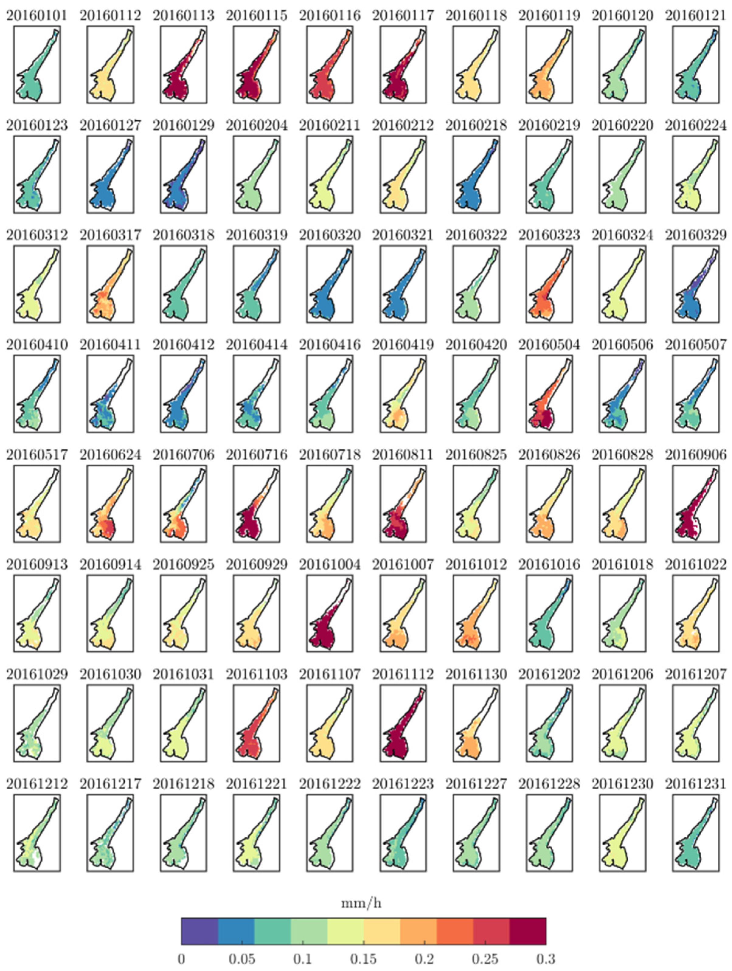
Figure 4 presents an example of the instantaneous evaporation maps that can be obtained with the LakeVap tool from CCI-Lakes LSWT maps and WRF meteorological data in one year. We chose to report the results from 2016 for which 80 images were available with irregular frequency, depending on the availability of satellite-derived LSWT maps. As the figure clearly shows, some maps are not complete, and white pixels cover those areas masked by clouds and/or where the quality of the LSWT product is too low. The time series allows the observation of the seasonal evolution of evaporation. Evaporation in Lake Garda typically increases from the beginning of the year until July to September, when the difference between air and water temperature is maximum, and then decreases again in late autumn and winter. This behavior is found every year and is related to the seasonal evolution of LSWT and to the thermal capacity of the lake, which stores heat during days of intense solar radiation and then slowly gives it off in the following days and months. However, exceptions to this trend can be occasionally found and are also visible in Figure 4. Unexpected maxima in winter (January), early spring (March, April), or late autumn (November) can be found when strong synoptic winds sweep over the lake enhancing evaporation, often associated with exceptionally cool and dry days when air temperature and relative humidity are much lower than the mean climatological conditions. Apart from these exceptions, evaporation maximum most often occurs in August (~45% of the analyzed years), while lower rates of evaporation are estimated from winter to spring, with the minimum often registered in March (~40% of the years). The yearly maximum of instantaneous evaporation typically ranges between 0.2 and 0.6 mm/h (spatially averaged value), and the minimum is between 0.01 and 0.05 mm/h. Spatial gradients up to the order of 0.05 mm/h can be observed between the northern and the southern part of the lake (see Section 3.4 for insight into the spatial patterns of instantaneous evaporation). In terms of daily evaporation rates (not shown), maximum values over the lake in one year range from 5.48 to 13.75 mm/day, while minimum values range from 0.15 to 1.61 mm/day.

3.2. Validation of LakeVap Products with Delft3D Outputs

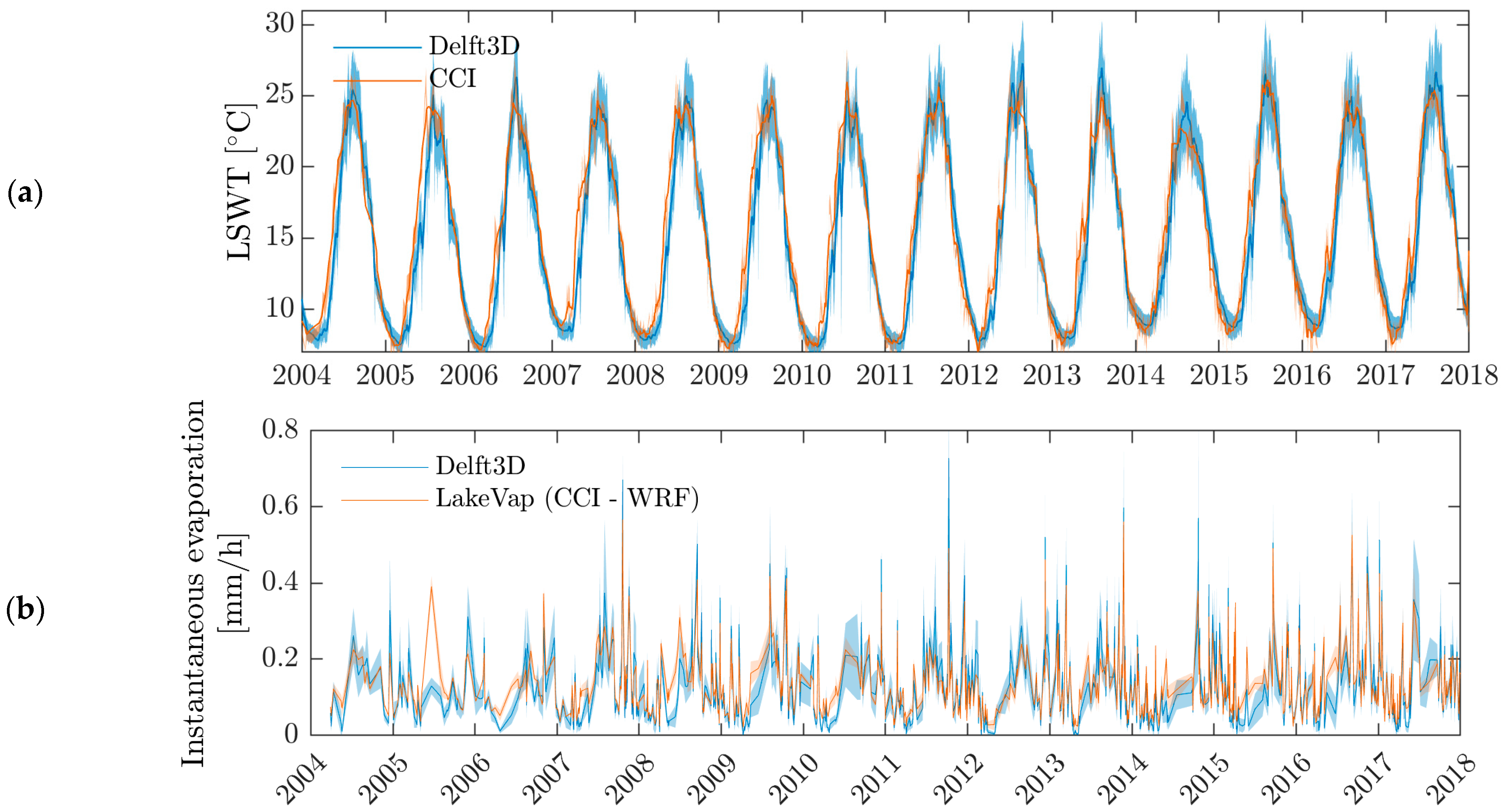
To validate the evaporation rates estimated with the LakeVap tool, we compare the instantaneous values ( E h ) obtained using different spatially averaged meteorological data against those estimated by the Delft3D model of Lake Garda by [35]. Figure 5a shows the time series of instantaneous evaporation rates obtained using the LakeVap tool fed with WRF meteorological data and the corresponding Delft3D evaporation estimates for the matching dates along the 2004–2018 long run of the Delft3D model. In Figure 5b, the time series of LSWT derived from the CCI-Lakes dataset and the one simulated by the Delft3D hydrodynamic model are compared.
In Table 3, we report the metrics displaying the performances of the LakeVap tool fed with different meteorological datasets as well as the metrics of the comparison between the two LSWT time series (last row of the table). The reference for evaporation values is the time series of instantaneous evaporation modeled via the previously validated Delft3D model.
Figure 5a shows that the two models provide the same order of magnitude of instantaneous evaporation (mean ± standard deviation of 0.129 ± 0.081 and 0.12 ± 0.098 for LakeVap and Delft3D, respectively) and have a synchronous seasonal behavior, with minima during winter/spring and peaks in summer/early autumn. The two evaporation time series thus have a high value of correlation (0.92) and a high value of NSE (0.834). The RMSD (0.04) is half of the standard deviation of the entire dataset, while the bias registered is very low (0.006) compared to the mean evaporation value of the time series. The good agreement between the Delft3D and LakeVap time series is explained by the similar approach used for computing the evaporation—i.e., the Dalton law. Both models indeed compute evaporation as an indirect function of the difference between air temperature and water temperature, whose peak occurs typically in late summer in Lake Garda. The spiky behavior of the standard deviation of Delft3D (light blue shaded area in Figure 5a) is related to the higher temporal frequency of the hydrodynamic model data, which are available daily. The two LSWT time series (Figure 5b) are strongly correlated (0.906) and show a high NSE (0.906), and the RMSE of 1.745 °C is relatively small compared to the range of LSWT (standard deviation of ±5.75 °C from CCI-Lakes database). The latter tends to be 0.5 °C warmer than the simulated water temperature, which is consistent with what was observed by the authors during the calibration and validation of the model against remotely sensed data from multiple sensors datasets (e.g., Landsat8, AVHRR, MODIS-Aqua, see [35], MODIS-Terra, see [57]).
Looking at Table 3, we can see that the performance of LakeVap strongly depends on the source of the atmospheric variables. With the use of ERA5 meteorological data, instantaneous evaporations are strongly underestimated (bias of −0.045 mm/h), while they gradually become more similar to the Delft3D estimates if meteorological variables are taken from the weather station MET1 and MET2. Among the two meteorological stations, the best performances are achieved with MET2, which is more representative of the mean lake weather conditions than MET1 and is more consistent with WRF data.

3.3. Implications of the Use of Different Meteorological Datasets

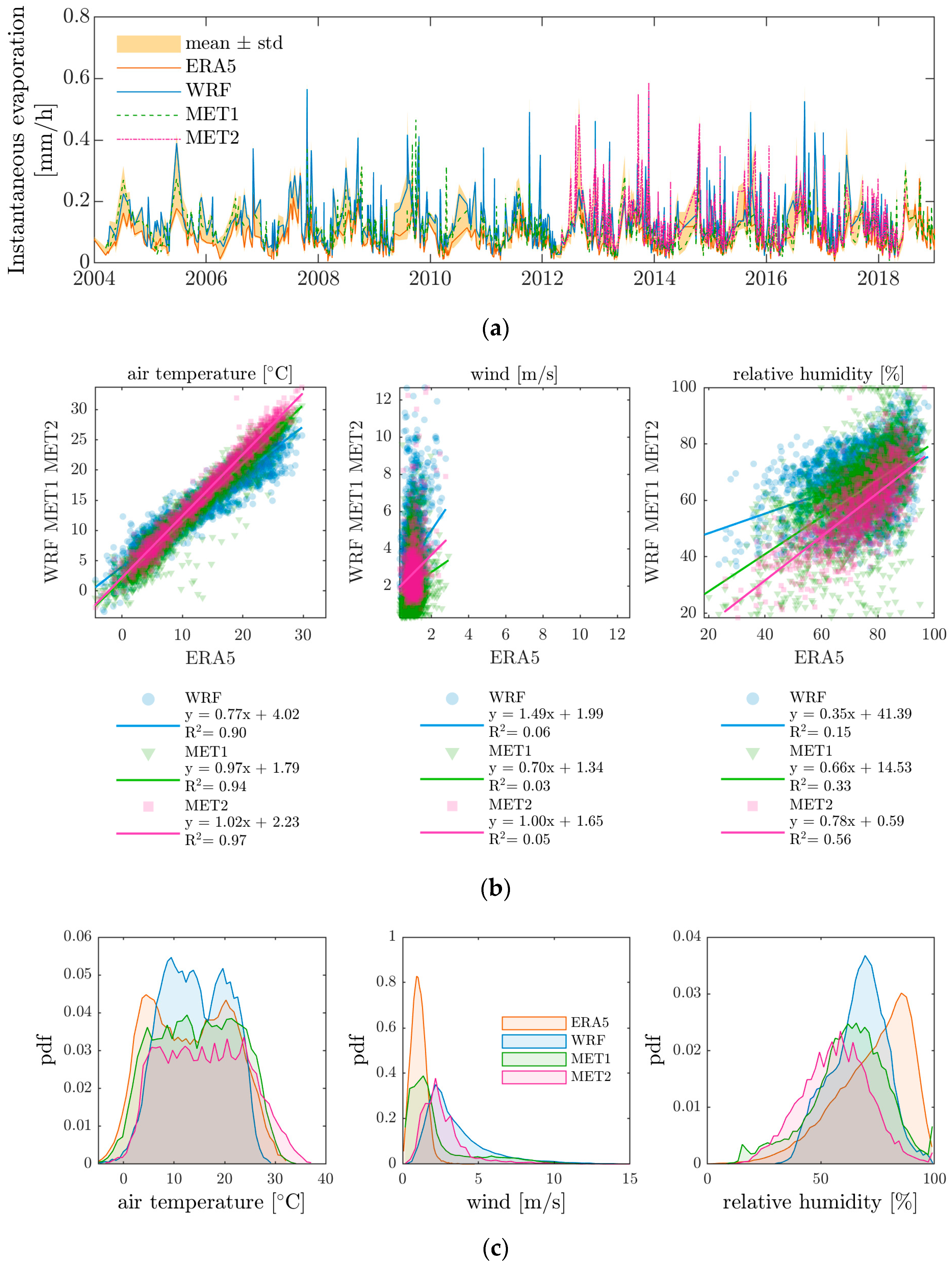
The results presented in Table 3 show that despite the seasonal behavior of the evaporation estimates from LakeVap being mainly driven by LSWT, the performance of the model is sensitive to weather data. Here, we deepen the analysis by presenting the results of the LakeVap tool combined with all available meteorological sources. In Figure 6a, the LakeVap tool results are presented as four time series of mean instantaneous evaporation ( E h ) rates obtained by using ERA5, MET1, MET2, and WRF data.
All four curves follow a similar behavior because the same LSWT drives the seasonal evaporation. While the minima of the time series are most often coherent, the peaks are more sensitive to the meteorological forcing used, with ERA5 giving the lowest evaporation values, followed by MET1, MET2 in-situ stations, and WRF (refer to Table 3 for the numerical values of mean ± standard deviation of the mentioned time series). The standard deviation associated with the different meteorological sources is on average 0.0352 mm/h over the entire period, with minima of the order of 0.0001 mm/h and maxima of the order of 0.1 mm/h. The order of magnitude of the latter coincides with that of the estimated instantaneous evaporation; hence, in some cases, the use of a different meteorological forcing leads to an over/underestimation of the evaporation rate by 100%. This is also visible in Figure 6a, where some of the peaks of the LakeVap + WRF time series are two times higher than those of LakeVap + ERA5. The meteorological datasets WRF, MET1, and MET2 are compared to ERA5 in Figure 6b. Air temperature is consistent between all datasets, with WRF, MET1, and MET2 showing a very clear correlation (R2 > 0.9) from all linear regressions. This is also confirmed by the frequency distribution of air temperatures from the four datasets in Figure 6c, which are all centered around the mean value between 13 °C and 16 °C with a similar standard deviation (~±8 °C for ERA5, MET1, MET2 and ±6.35 °C for WRF). WRF air temperature shows a smaller standard deviation than in-situ and ERA5 data, which implies that the model tends to reproduce colder summer peaks and warmer winter cooling. It is worth noting that the WRF model tends to underestimate air temperature in MET1 and MET2, as already pointed out by [35]. However, it is also known that WRF is usually better aligned with MET2 than MET1, as the high spatial heterogeneity of the lake also causes discrepancies between the different in-situ weather stations. As clearly depicted in Figure 6c, the curve of MET2 is more shifted towards warm temperatures than MET1, which tends to register colder winter temperatures and milder summers. Wind speed from WRF, MET1, and MET2 is largely higher than ERA5 wind speed, with the highest values found in WRF and MET2. No correlation is visible between the three datasets and ERA5 (R2 < 0.1). The frequency distribution curve of ERA5 wind speed in Figure 6c is centered on smaller values and is less spread, which shows not only an underestimation of the wind speed but also a reduced variability of this quantity. The mean value of ERA5 wind speed in the investigated dates is indeed 1 (±0.48) m/s, which is two times smaller than that of MET1 and MET2 (2.17 ± 2.21 m/s and 2.66 ± 1.59 m/s, respectively) and three times smaller than that of WRF (3.53 ± 2.18 m/s). It is worth noting that significant differences are also visible between the three curves from WRF, MET1, and MET2, but a good agreement is found between WRF and MET2, which is consistent with what was already observed by [35]. Among the four datasets, relative humidity is more consistent than wind speed but less than the air temperature, with correlation still low (0.15 < R2 < 0.6 from the regression lines) and significant differences in either mean values and spread of the distribution curves. ERA5’s relative humidity tends to be the highest, which is surprising considering the amount of land included in the model grid cells, followed by WRF, MET1, and MET2. In this case, relative humidity from WRF is more consistent with that of MET1. Differences between MET1 and MET2 can be explained by the position of the meteorological station, with MET1 being directly on the wharf, while MET2 is on solid ground.

3.4. Spatial Variability of Evaporation

In the above sections, we have shown how evaporation estimates are sensitive to the meteorological forcing considering the evaporation in spatially averaged terms. However, the LakeVap tool produces maps of evaporation whose spatial variability can be interpreted based on the spatial variability of both LSWT and atmospheric variables, if those are imposed as space and time-varying fields. In this section, we interpret the relative weight of each meteorological variable in affecting the spatial variability of evaporation.
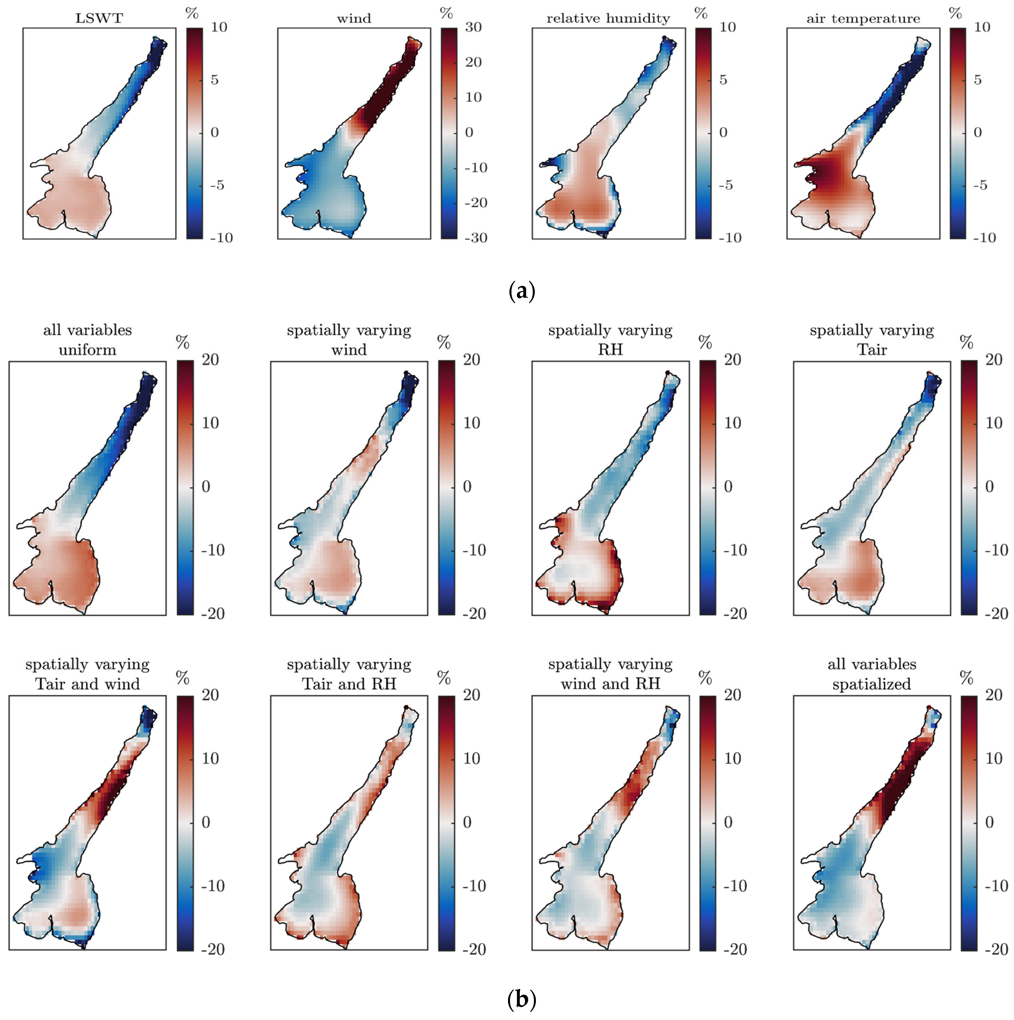
In Figure 7, we present the results from sensitivity tests performed to investigate this aspect, as previously detailed in Section 2.4.
The maps in the panels depict the normalized anomaly Δ X estimated as in Equation (8), which represents the mean (in time) percentage spatial variation of a given quantity. In Figure 7a, we report the normalized anomaly of the inputs of the model, i.e., LSWT, wind speed, air temperature, and relative humidity, while in Figure 7b, the normalized anomaly is calculated for E h obtained from the different LakeVap sensitivity tests.
LSWT, wind, and air temperature normalized anomalies in Figure 7a clearly show that longitudinal gradients are typical in Lake Garda. Air and water temperatures indeed tend to be warmer in the southern part and colder in the northern part, where stronger winds typically develop due to thermal breezes from north to south at the acquisition time of CCI-Lakes dataset sensors (i.e., morning around 10:00 UTC). Air temperature variability is double that of LSWT: the spatial gradients of LSWT reach −4/+8% (10th/90th percentiles) while those of air temperature reach −8/+19% throughout the year. The order of magnitude of wind spatial variability is much higher, with winds up to 30% stronger in the north and down to 20% weaker in the south, on average, and with maximum/minimum variations above ±50%. The spatial variability of relative humidity depends on the morphology of the lake and does not vary in time, such that the order of magnitude of average patterns is the same as the extremes of the distribution in time: higher/lower humidity (up to ±10%) is registered in the central part of the lake and close to the shores, respectively.
Figure 7b shows that the first driver of spatial patterns of the LakeVap results is LSWT, which is the minimum requisite for the model to produce evaporation maps. The spatial pattern of E h resembles that of LSWT if all meteorological variables are taken as spatially averaged, while different patterns can be found if one or more atmospheric forcing is spatially distributed. Since wind anomalies have opposite patterns with respect to LSWT, the evaporation pattern resulting from applying spatially varying wind fields consists of regions of positive anomalies induced by the dominant forcing in that area. Evaporation is higher in the northern part, which is colder but subject to stronger winds, and in the southern shallow part, where winds are mild but temperatures tend to be higher. The effect of spatially varying relative humidity and air temperature is less significant in the lake, as both variables are inversely proportional to evaporation, such that those areas that were associated with positive anomalies in Figure 7a are now related to smaller variations in evaporation and vice versa. In particular, air temperature causes a general smoothing of spatial variability: in fact, the air temperature has the same spatial pattern as LSWT; hence, high evaporation rates tend to be prevented in the warmer areas of the lake, where the gradient between air and water is reduced, and the same occurs in the areas of negative anomalies. When summing up the contributions of two or more atmospheric variables, the spatial distribution of evaporation progressively changes. E h estimated with the LakeVap tool using all WRF spatialized meteorological fields shows a spatial variation of the order of +20% in the northern part of the lake and of −5% in the other regions. This variation comes as an average over the entire time series with maximum/minimum variations exceeding ±30% (10th and 90th percentiles). The spatial pattern of the normalized evaporation anomaly shows a clear gradient along the main axis of the lake. Higher evaporation occurs along the central part of the northern trunk, with lower rates close to the northernmost part and in the southern basin. This spatial pattern is due to the concurring effect of high wind speeds, lower air temperature, and lower relative humidity in the northern basin, which lead to high evaporation rates despite the region typically showing colder LSWT. This pattern is the same obtained from the daily time series of instantaneous evaporation from the Delft3D model (not shown) and cannot be obtained when a single value for meteorological variables is used (e.g., from ERA5, MET1, MET2, or even spatially averaged WRF data), as it is a direct consequence of the space-varying field of LSWT and all relevant atmospheric forcings.

4. Discussion

4.1. Evaporation Estimates for Lake Garda

This study provides for the first time, to the best knowledge of the authors, instantaneous and daily evaporation estimates for Lake Garda. In 2008, a stable isotope analysis of the lake hydrological balance failed to estimate the yearly evaporation rate. The order of magnitude of instantaneous (0.1 ± 0.08 mm/h) and daily (3.1 ± 1.92 mm/day) evaporation estimated from the entire LakeVap time series (with WRF spatially averaged forcing) is consistent with the estimations/direct measurements of latent heat flux in lakes similar to Lake Garda (e.g., Lake Constance, where [49] found the same seasonal behavior with maxima in August and minima in March; Lake Geneva [22,67]).
The seasonal evolution of evaporation from Lake Garda is mainly driven by the thermal gradients between air and water (as in [68]). Exceptions to the typical seasonal values are associated with unexpected climatic conditions (e.g., synoptic-scale wind events, exceptional cool or warm days [8,9,23]). As in [23], such exceptions are associated with lake-wide higher/lower evaporation rates. We have seen that this also occurs in Lake Garda in the example year 2016 reported in Figure 4.
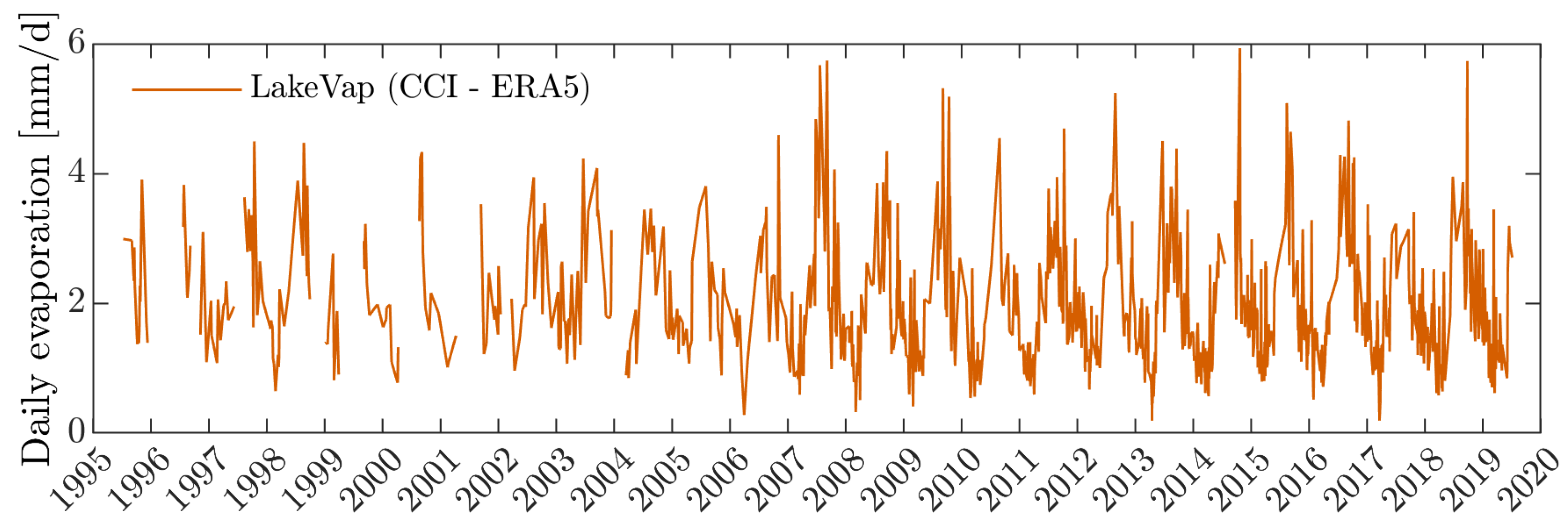
We have shown that the LakeVap tool allows the generation of instantaneous and daily evaporation maps of water bodies for relatively long time series, depending on the revisiting time of sensors sensitive to thermal bands. LakeVap evaporation products are hence first limited by the EO data availability, and in particular, (1) the operativity and the revisiting time of passive satellites, from which LSWT products are derived, and (2) the cloud coverage conditions during the satellite acquisitions. Thanks to the efforts of the CCI-Lakes project, it is possible to have a homogenized and long time series of LSWT products for 250 lakes in version 1 and 2000 lakes in version 2. This was possible thanks to the exploitation and integration of different sensor acquisitions over the years [69]. The integration of different sensor products increases the frequency of EO acquisitions, and the progressive launch of newer and more technologically advanced sensors allows an increase in both the frequency and quality of the LSWT product. The second requirement of LakeVap is a comprehensive dataset of meteorological variables. Thanks to the availability of global meteorological datasets, such as ERA5 tested in this study, long-term evaporation rates can be estimated. In the case presented here, ERA5 covers the entire period of availability of CCI-Lakes LSWT maps for Lake Garda; hence, its use within LakeVap allows the evaluation of the evolution of evaporation rates over 25 years, as reported in Figure 8. The figure clearly shows the interannual and seasonal variation of evaporation rates in Lake Garda and is consistent with what was already presented in the results on an hourly basis (e.g., in Figure 5a and Figure 6a).
Gaps are more frequent in the first years of the time series, when fewer sensors were operational for the retrieval of LSWT and available maps are mainly from summer to winter days. The average number of LSWT maps acquired annually during the period 1995–2006 is 19, while that from the period 2007–2019 is 74. Such a discrepancy is due to the operativity of the AVHRR sensor which was launched onboard the Metop satellite at the end of 2006 (CCI-LAKES-0029-PUG (https://climate.esa.int/media/documents/CCI-LAKES-0029-PUG_v1.1_signed_CA.pdf, accessed on 28 April 2022)). A similar time series can be obtained for any case study included in datasets such as CCI-Lakes without the need for additional information, as global atmospheric/land models have worldwide coverage.

4.2. Sensitivity to Meteorological Forcing and Morphological Complexity of the Test Site

In Section 3.3, we have seen that the estimated evaporation depends on the meteorological forcing adopted, as also highlighted by [34]. Our results show that the ERA5 dataset tends to underestimate the wind speed and overestimate the relative humidity (Figure 6), leading to an overall underestimation of the evaporation compared to the reference estimates from the Delft3D model (Table 3).
Based on a sensitivity analysis (reported in the Supplementary Material S2), we found that a decrease of 50% of relative humidity can lead to an increase of 100% of evaporation, but the relative humidity has been observed to vary around ±20% in our realistic simulations covering 14 years and is generally better predicted by ERA5. As for the wind speed, we found that an increase of 50% in wind speeds leads on average to an increase of 25% in evaporation. Even if wind speed variations impact the evaporation estimates relatively less than the relative humidity, in absolute terms, the effective weight of such variations is heavier on evaporation because wind is more variable in space in our test site (up to 100%) and is more difficult to predict by global models as ERA5. In this regard, we recall that ERA5 is a global dataset and has a coarse resolution (0.1° lat/lon, corresponding to 11 km approximately); hence, it ensures a limited description of the complex topography of the surrounding region, while WRF and in-situ data are more representative of the specific lake conditions. This is clear if the spatial resolution of ERA5 and WRF is compared in Figure 3b. The different cell resolution complicates the direct comparison between the two models as well as between them and in-situ data from MET1 and MET2. From each model, the points inside the lake were averaged to obtain a single value for each variable to feed the LakeVap tool. Thus, the final value of the single atmospheric variable comes from an average of 94 points for the WRF grid and 4 points for ERA5, while it is representative of the exact location of the weather station for MET1 and MET2. It is also worth noting that, in our analysis, we selected in-lake points only from ERA5 and WRF datasets. This led to the exclusion of those ERA5 points that were potentially more representative of the northern-basin atmospheric conditions (see Figure 3b), where wind speeds are generally higher and air temperature and relative humidity lower (see e.g., Figure 7a). This selection likely concurred with the general underestimation of evaporation rates obtained with the ERA5 dataset.
The comparison between in-situ measured (MET1 and MET2) and model-derived (ERA5 and WRF) meteorological variables for Lake Garda also demonstrates that it is difficult to find a meteorological source that works best because even in-situ meteorological stations (MET1 and MET2) are not perfectly consistent each other (Figure 6). This is due to the particular morphology of Lake Garda, which is subject to the canalization of wind currents in the northern part of the lake and thus to strong gradients of air temperature and relative humidity between the northern and southern sub-basins. Thus, evaporation patterns tend to follow the patterns of air masses traveling over the lake [23]. A significant longitudinal gradient exists in LSWT patterns as well. LSWT heterogeneity drives the evaporation pattern if uniform meteorological forcing is used (Figure 7). We have seen in this regard that the choice of a single value representing the atmospheric conditions of the entire lake might not be the best option if evaporation is intended to be analyzed in terms of spatial gradients. Our results show that if all atmospheric variables are considered as space varying, the area that evaporates the most in Lake Garda is located in the northern part of the lake, where air temperature and relative humidity are lower, the wind is faster, and the lake water is colder. This result reverses the LSWT-driven spatial pattern, which instead shows that the most evaporating part is the southern basin, which is shallower and generally warmer. A key role in this regard is played by the wind, which increases by 10% (on a time average) the spatial variability of the predicted evaporation. This is consistent with existing studies on lakes of the size and morphology similar to Lake Garda. In Lake Geneva [22,24] stressed how important spatial variability is for determining the heat budget of a lake. In particular, the authors of [24] ascribed to wind patterns most of the spatial variability of surface heat fluxes from summer to winter.
However, the seasonal and interannual trends of evaporation can be still evaluated by considering the spatially averaged evaporation from the lake. This quantity is well predicted by the LakeVap tool also if uniform meteorological data are provided. The constraint to this is that such uniform values have to be representative of the average atmospheric conditions over the lake (Table 3 and Figure 6). In the case of the absence of in-situ data for such verification, the combination of the LakeVap tool with global datasets of LSWT (e.g., CCI-Lakes) and meteorological quantities (e.g., ERA5) provides at least a quantitative estimate of the order of magnitude of instantaneous and daily evaporation and of the daily heat balance (Figure 8).

4.3. The LakeVap Tool and Applicability to Other Lakes

In this contribution, we present an easy-to-use and fast tool for the production of evaporation maps on an instantaneous and daily basis which can be potentially used without the need for any in-situ data. The chosen formulation follows simple equations of heat balance which are available in any physical limnology and oceanography manual. For the latent heat flux from which evaporation is derived, we followed a classical Dalton law. For the parameterization of the wind function, we followed the approach proposed by [49], who in turn applied to Lake Constance the formulas proposed for Lake Ägeri by [50] and for Lake Zurich by [70]. We assumed that these lakes have sufficient similarities to Lake Garda and alpine lakes of the same morphological and climatological features, but further investigations should be conducted to verify such assumptions in our and other study cases, ideally where direct measurements are available. We note in this regard that direct measurements of evaporation are still a rarity among in-situ data and are not available for our test site. For this reason, we validated the LakeVap estimates against a validated hydro-thermodynamic model which was demonstrated to correctly reproduce the heat balance in Lake Garda [35]. The agreement between LakeVap and Delft3D models is promising since, despite the similar approach in the computation of evaporation rates, the input data required and the costs of the two models are extremely different. While Delft3D solves complex three-dimensional hydrodynamic equations and calculated the heat fluxes based on atmospheric simulations, LakeVap only requires LSWT from satellite acquisitions and meteorological data from a single source. Hence, the LakeVap tool represents a useful alternative to expensive and time-demanding models for estimating evaporation and allows for a quantification of water loss due to evaporation rates in those lakes and reservoirs where in-situ measurements are still not available or impossible.
While existing RS-based methods (e.g., SEBAL, METRIC, SEBS) were formulated for evapotranspiration and then, in some cases, eventually extended to inland water bodies, LakeVap is specifically formulated for estimating evaporation from water surfaces. By using LSWT, the issues related to the heat capacity of the lake are overcome. At the instantaneous rate, the LSWT is already affected by the thermal inertia of the lake, and thus the hourly evaporation intrinsically considers this effect. At the daily rate, the simplified heat balance uses the net heat Q x , t to cool or warm the LSWT, while evaporation is simply computed by following the Dalton approach and accumulated at every hourly iteration. Thus, in contrast to other RS-based methods, the application of LakeVap to any lake or reservoir is immediate and does not require any specific assumption. The coefficients of the wind function must, however, be carefully checked, in order to parameterize the effect of wind in the correct way for the study site. In this regard, the advantages and constraints of the approach behind LakeVap are the same of existing mass transfer or bulk transfer methods specified in Table 1.
Thanks to its flexibility and easy handling, the LakeVap tool can be integrated into infrastructures supporting the management of water reservoirs. If applied to dammed lakes devoted to the production of hydroelectricity, dam managers could assess water losses due to evaporation and consequently tune the water withdrawal to have the maximum proficiency and the minimum waste of the water resource. Furthermore, the combination of water evaporation volumes with the plant energy production of a dam provides the blue water footprint of the reservoir [71], and this is a way to quantify the impact of the “consuming” capacity of a hydropower system on the production of energy. This is particularly relevant in situations of water scarcity such as arid and semi-arid environments [14]. In addition, with the frequency and intensity of heatwaves set to increase, which can hit urban areas more severely [72,73], nearby water bodies may become a vital mitigating component. Lakes and rivers have been shown to have a significant cooling effect on the nearby urban environment through evaporation using Landsat imagery [74]. However, given the increase in atmospheric stilling in recent decades [2], the lower wind speeds may reduce the potential for this. There are also likely to be applications in ecological management as evaporation contributing to a significant decrease in the water level can also alter the light climate in the littoral zone of lakes. This would be particularly important in the south of Lake Garda, where a delicate ecological balance is maintained between submerged aquatic plants, supporting an overwintering waterfowl population ranked the most diverse and abundant in Italy [75,76]. Finally, the dependence of the LakeVap tool on any type of satellite-derived LSWT data gives the possibility to enlarge its applicability to even medium-small sized water bodies exploiting the relatively high spatial resolution (30 m) of Landsat sensors.

5. Conclusions

The main purpose of this contribution is to present and test the LakeVap tool for the estimation of instantaneous evaporation rates in a relatively complex lacustrine environment where such information is already available from a validated and far more complex hydro-thermodynamic model. The EO-based model LakeVap estimates evaporation from water surfaces by requiring as inputs LSWT maps and a few meteorological variables (i.e., air temperature, wind speed, air relative humidity, and solar radiation). The model handles single (averaged) meteorological information as well as spatialized data and produces instantaneous or daily evaporation maps of the case study. In this contribution, the application to Lake Garda produced estimates comparable to the outputs of a complex hydro-thermodynamic model specifically calibrated for the lake and consistent with the evaporation estimates for similar lakes. We also showed that the choice of the input meteorological variables can significantly affect the evaporation estimation, up to doubling or halving the instantaneous evaporation rates in some cases. Furthermore, the key meteorological variables impact the evaporation estimates in different ways. Among them, the wind speed was found to be the variable that varies the most and has the greatest effect on the estimation of evaporation in Lake Garda. Evaporation maps for Lake Garda were interpreted based on the spatial variation of meteorological variables and LSWT, which together contribute to the definition of the spatial patterns of evaporation from the lake surface. The specific morphology of Lake Garda causes a great heterogeneity in both atmospheric conditions and LSWT. This heterogeneity makes the choice of a single value for representing the entire lake conditions not as straightforward as it can be in smaller or more regularly shaped lakes, where the use of data either coming from space-averaged model data or a single in-situ station can provide a good approximation of the meteorological forcing involved in the evaporation process. In this regard, the LakeVap tool has the potential to be applied to every natural or manmade water body on the Earth as long as its shape and its extension can be mapped by thermal sensors providing LSWT maps.

Supplementary Materials

The following supporting information can be downloaded at https://www.mdpi.com/article/10.3390/rs14112636/s1. Refs. [27,49,50,51,77,78] are cited in the supplementary materials. The Supplementary materials include Section S1: Heat balance equation and Table S1: list of symbols; Section S2: Sensitivity of evaporation estimates to meteorological variables and Figure S1: results of sensitivity tests.

Author Contributions

Conceptualization, E.M., M.A., M.B. and C.G.; Methodology, E.M., M.A.; Software, E.M.; Formal analysis, M.A.; Writing—original draft., E.M., M.A.; Writing—review and editing, M.B., C.G. and G.F.; Funding acquisition, C.G., M.B. All authors have read and agreed to the published version of the manuscript.

Funding

This work was supported by the EU Horizon 2020 program with the projects HYPOS (GA No. 870504) and Water-ForCE (GA No. 101004186) and by the ESA CCI LAKES project (GA No. 40000125030/18/I-NB).

Acknowledgments

We thank the European Centre for Medium-Range Weather Forecast (ECMWF), the Environmental Protection Agency of Lombardia Region (ARPA-Lombardia) and the Edmund Mach Foundation (FEM) for providing meteorological data. We are also grateful to Lorenzo Giovannini (UniTN) for running the WRF simulation and sharing their results. We are very grateful to R. Colombo, A. De Carli, I. Cazzaniga, and C. Elli for their support in developing this study over the years and to K. Schenk and H. Bernert for the testing of the code.

Conflicts of Interest

The authors declare no conflict of interest.

Code Availability

The code of the LakeVap tool is available upon request.

References

  1. Wang, W.; Lee, X.; Xiao, W.; Liu, S.; Schultz, N.; Wang, Y.; Zhang, M.; Zhao, L. Global Lake Evaporation Accelerated by Changes in Surface Energy Allocation in a Warmer Climate. Nat. Geosci. 2018, 11, 410–414. [Google Scholar] [CrossRef]
  2. Woolway, R.I.; Merchant, C.J.; Van Den Hoek, J.; Azorin-Molina, C.; Nõges, P.; Laas, A.; Mackay, E.B.; Jones, I.D. Northern Hemisphere Atmospheric Stilling Accelerates Lake Thermal Responses to a Warming World. Geophys. Res. Lett. 2019, 46, 11983–11992. [Google Scholar] [CrossRef] [Green Version]
  3. Vystavna, Y.; Harjung, A.; Monteiro, L.R.; Matiatos, I.; Wassenaar, L.I. Stable Isotopes in Global Lakes Integrate Catchment and Climatic Controls on Evaporation. Nat. Commun. 2021, 12, 7224. [Google Scholar] [CrossRef] [PubMed]
  4. Zhou, W.; Wang, L.; Li, D.; Leung, L.R. Spatial Pattern of Lake Evaporation Increases under Global Warming Linked to Regional Hydroclimate Change. Commun. Earth Environ. 2021, 2, 255. [Google Scholar] [CrossRef]
  5. Peel, M.C.; Finlayson, B.L.; McMahon, T.A. Updated World Map of the Köppen-Geiger Climate Classification. Hydrol. Earth Syst. Sci. 2007, 11, 1633–1644. [Google Scholar] [CrossRef] [Green Version]
  6. Maberly, S.C.; O’Donnell, R.A.; Woolway, R.I.; Cutler, M.E.J.; Gong, M.; Jones, I.D.; Merchant, C.J.; Miller, C.A.; Politi, E.; Scott, E.M.; et al. Global Lake Thermal Regions Shift under Climate Change. Nat. Commun. 2020, 11, 1232. [Google Scholar] [CrossRef]
  7. Riveros-Iregui, D.A.; Lenters, J.D.; Peake, C.S.; Ong, J.B.; Healey, N.C.; Zlotnik, V.A. Evaporation from a Shallow, Saline Lake in the Nebraska Sandhills: Energy Balance Drivers of Seasonal and Interannual Variability. J. Hydrol. 2017, 553, 172–187. [Google Scholar] [CrossRef] [Green Version]
  8. Blanken, P.D.; Spence, C.; Hedstrom, N.; Lenters, J.D. Evaporation from Lake Superior: 1. Physical Controls and Processes. J. Great Lakes Res. 2011, 37, 707–716. [Google Scholar] [CrossRef]
  9. Xiao, K.; Griffis, T.J.; Baker, J.M.; Bolstad, P.V.; Erickson, M.D.; Lee, X.; Wood, J.D.; Hu, C.; Nieber, J.L. Evaporation from a Temperate Closed-Basin Lake and Its Impact on Present, Past, and Future Water Level. J. Hydrol. 2018, 561, 59–75. [Google Scholar] [CrossRef]
  10. Yang, K.; Lu, H.; Yue, S.; Zhang, G.; Lei, Y.; La, Z.; Wang, W. Quantifying Recent Precipitation Change and Predicting Lake Expansion in the Inner Tibetan Plateau. Clim. Chang. 2018, 147, 149–163. [Google Scholar] [CrossRef]
  11. Guo, Y.; Zhang, Y.; Ma, N.; Xu, J.; Zhang, T. Long-Term Changes in Evaporation over Siling Co Lake on the Tibetan Plateau and Its Impact on Recent Rapid Lake Expansion. Atmos. Res. 2019, 216, 141–150. [Google Scholar] [CrossRef]
  12. Elsawwaf, M.; Willems, P.; Feyen, J. Assessment of the Sensitivity and Prediction Uncertainty of Evaporation Models Applied to Nasser Lake, Egypt. J. Hydrol. 2010, 395, 10–22. [Google Scholar] [CrossRef]
  13. Bozorgi, A.; Bozorg-Haddad, O.; Sima, S.; Loáiciga, H.A. Comparison of Methods to Calculate Evaporation from Reservoirs. Int. J. River Basin Manag. 2020, 18, 1–12. [Google Scholar] [CrossRef]
  14. Friedrich, K.; Grossman, R.L.; Huntington, J.; Blanken, P.D.; Lenters, J.; Holman, K.D.; Gochis, D.; Livneh, B.; Prairie, J.; Skeie, E.; et al. Reservoir Evaporation in the Western United States: Current Science, Challenges, and Future Needs. Bull. Am. Meteorol. Soc. 2018, 99, 167–187. [Google Scholar] [CrossRef]
  15. Sene, K.; Gash, J.; McNeil, D. Evaporation from a Tropical Lake: Comparison of Theory with Direct Measurements. J. Hydrol. 1991, 127, 193–217. [Google Scholar] [CrossRef]
  16. Rosenberry, D.O.; Winter, T.C.; Buso, D.C.; Likens, G.E. Comparison of 15 Evaporation Methods Applied to a Small Mountain Lake in the Northeastern USA. J. Hydrol. 2007, 340, 149–166. [Google Scholar] [CrossRef]
  17. Ali, S.; Ghosh, N.C.; Singh, R. Evaluating Best Evaporation Estimate Model for Water Surface Evaporation in Semi-Arid Region, India. Hydrol. Process 2008, 22, 1093–1106. [Google Scholar] [CrossRef]
  18. Alazard, M.; Leduc, C.; Travi, Y.; Boulet, G.; Ben Salem, A. Estimating Evaporation in Semi-Arid Areas Facing Data Scarcity: Example of the El Haouareb Dam (Merguellil Catchment, Central Tunisia). J. Hydrol. Reg. Stud. 2015, 3, 265–284. [Google Scholar] [CrossRef] [Green Version]
  19. Majidi, M.; Alizadeh, A.; Farid, A.; Vazifedoust, M. Development and Application of a New Lake Evaporation Estimation Approach Based on Energy Balance. Hydrol. Res. 2018, 49, 1528–1539. [Google Scholar] [CrossRef]
  20. Lowe, L.D.; Webb, J.A.; Nathan, R.J.; Etchells, T.; Malano, H.M. Evaporation from Water Supply Reservoirs: An Assessment of Uncertainty. J. Hydrol. 2009, 376, 261–274. [Google Scholar] [CrossRef]
  21. Wang, W.; Xiao, W.; Cao, C.; Gao, Z.; Hu, Z.; Liu, S.; Shen, S.; Wang, L.; Xiao, Q.; Xu, J.; et al. Temporal and Spatial Variations in Radiation and Energy Balance across a Large Freshwater Lake in China. J. Hydrol. 2014, 511, 811–824. [Google Scholar] [CrossRef]
  22. Rahaghi, A.I.; Lemmin, U.; Cimatoribus, A.; Bouffard, D.; Riffler, M.; Wunderle, S.; Barry, D.A. Improving Surface Heat Flux Estimation for a Large Lake through Model Optimization and Two-Point Calibration: The Case of Lake Geneva. Limnol. Oceanogr. Methods 2018, 16, 576–593. [Google Scholar] [CrossRef]
  23. Spence, C.; Blanken, P.D.; Hedstrom, N.; Fortin, V.; Wilson, H. Evaporation from Lake Superior: 2. Spatial Distribution and Variability. J. Great Lakes Res. 2011, 37, 717–724. [Google Scholar] [CrossRef]
  24. Rahaghi, A.I.; Lemmin, U.; Cimatoribus, A.A.; Barry, D.A. The Importance of Systematic Spatial Variability in the Surface Heat Flux of a Large Lake: A Multiannual Analysis for Lake Geneva. Water Resour. Res. 2019, 55, 10248–10267. [Google Scholar] [CrossRef] [Green Version]
  25. Bastiaanssen, W.G.M.; Menenti, M.; Feddes, R.A.; Holtslag, A.A.M. A Remote Sensing Surface Energy Balance Algorithm for Land (SEBAL). 1. Formulation. J. Hydrol. 1998, 212–213, 198–212. [Google Scholar] [CrossRef]
  26. Bastiaanssen, W.G.M.; Pelgrum, H.; Wang, J.; Ma, Y.; Moreno, J.F.; Roerink, G.J.; Van Der Wal, T. A Remote Sensing Surface Energy Balance Algorithm for Land (SEBAL).: Part 2: Validation. J. Hydrol. 1998, 212–213, 213–229. [Google Scholar] [CrossRef]
  27. Allen, R.G.; Tasumi, M.; Trezza, R. Satellite-Based Energy Balance for Mapping Evapotranspiration with Internalized Calibration (METRIC)—Model. J. Irrig. Drain. Eng. 2007, 133, 380–394. [Google Scholar] [CrossRef]
  28. Su, Z. The Surface Energy Balance System (SEBS) for Estimation of Turbulent Heat Fluxes. Hydrol. Earth Syst. Sci. 2002, 6, 85–100. [Google Scholar] [CrossRef]
  29. Allen, R.G.; Tasumi, M.; Morse, A.; Trezza, R.; Wright, J.L.; Bastiaanssen, W.; Kramber, W.; Lorite, I.; Robison, C.W. Satellite-Based Energy Balance for Mapping Evapotranspiration with Internalized Calibration (METRIC)—Applications. J. Irrig. Drain. Eng. 2007, 133, 395–406. [Google Scholar] [CrossRef]
  30. Amayreh, J. DigitalCommons @ USU All Graduate Theses and Dissertations Lake Evaporation: A Model Study. 1995. Available online: https://digitalcommons.usu.edu/etd/4404 (accessed on 28 April 2022).
  31. Hassan, M. Evaporation Estimation for Lake Nasser Based on Remote Sensing Technology. Ain Shams Eng. J. 2013, 4, 593–604. [Google Scholar] [CrossRef] [Green Version]
  32. Zamani Losgedaragh, S.; Rahimzadegan, M. Evaluation of SEBS, SEBAL, and METRIC Models in Estimation of the Evaporation from the Freshwater Lakes (Case Study: Amirkabir Dam, Iran). J. Hydrol. 2018, 561, 523–531. [Google Scholar] [CrossRef]
  33. Abdelrady, A.; Timmermans, J.; Vekerdy, Z.; Salama, M.S. Surface Energy Balance of Fresh and Saline Waters: AquaSEBS. Remote Sens. 2016, 8, 583. [Google Scholar] [CrossRef] [Green Version]
  34. Zhao, G.; Gao, H. Estimating Reservoir Evaporation Losses for the United States: Fusing Remote Sensing and Modeling Approaches. Remote Sens. Environ. 2019, 226, 109–124. [Google Scholar] [CrossRef] [Green Version]
  35. Amadori, M.; Giovannini, L.; Toffolon, M.; Piccolroaz, S.; Zardi, D.; Bresciani, M.; Giardino, C.; Luciani, G.; Kliphuis, M.; van Haren, H.; et al. Multi-Scale Evaluation of a 3D Lake Model Forced by an Atmospheric Model against Standard Monitoring Data. Environ. Model. Softw. 2021, 139, 105017. [Google Scholar] [CrossRef]
  36. McGuinness, J.L.; Bordne, E.F. A Comparison of Lysimeter-Derived Potential Evapotranspiration with Computed Values; U.S. Department of Agriculture: Washington, DC, USA, 1972; Volume Technical.
  37. Hargreaves, G.H. Moisture Availability and Crop Production. Trans. ASAE 1975, 18, 0980–0984. [Google Scholar] [CrossRef]
  38. Delclaux, F.; Coudrain, A.; Condom, T. Evaporation Estimation on Lake Titicaca: A Synthesis Review and Modelling. Hydrol. Process 2007, 21, 1664–1677. [Google Scholar] [CrossRef]
  39. Ward, A.D.; Trimble, S.W. Environmental Hydrology; Lewis: Boca Raton, FL, USA, 2003. [Google Scholar]
  40. Hamon, W.R. Estimating Potential Evapotranspiration. J. Hydraul. Div. 1961, 87, 107–120. [Google Scholar] [CrossRef]
  41. Hassani, A. Thermal Structure and Energy Budget for Alghadir Reservoir, Iran. Water Resour. 2013, 40, 621–630. [Google Scholar] [CrossRef]
  42. Aydin, H.; Karakuş, H. Estimation of Evaporation for Lake Van. Environ. Earth Sci. 2016, 75, 1275. [Google Scholar] [CrossRef]
  43. Singh, V.P.; Xu, C.-Y. Evaluation and Generalization of 13 Mass-Transfer Equations for Determining Free Water Evaporation. Hydrol. Process 1997, 11, 311–323. [Google Scholar] [CrossRef]
  44. Stewart, R.B.; Rouse, W.R. A Simple Method for Determining the Evaporation from Shallow Lakes and Ponds. Water Resour. Res. 1976, 12, 623–628. [Google Scholar] [CrossRef]
  45. De Bruin, H.A.R. A Simple Model for Shallow Lake Evaporation. J. Appl. Meteorol. 1978, 17, 1132–1134. [Google Scholar] [CrossRef] [Green Version]
  46. De Bruin, H.A.R.; Keijman, J.Q. The Priestley-Taylor Evaporation Model Applied to a Large, Shallow Lake in the Netherlands. J. Appl. Meteorol. 1979, 18, 898–903. [Google Scholar] [CrossRef] [Green Version]
  47. Brutsaert, W.; Stricker, H. An Advection-Aridity Approach to Estimate Actual Regional Evapotranspiration. Water Resour. Res. 1979, 15, 443–450. [Google Scholar] [CrossRef]
  48. Brutsaert, W. Evaporation into the Atmosphere; Springer: Dordrecht, The Netherlands, 1982; ISBN 978-90-481-8365-4. [Google Scholar]
  49. Fink, G.; Schmid, M.; Wahl, B.; Wolf, T.; Wüest, A. Heat Flux Modifications Related to Climate-Induced Warming of Large European Lakes. Water Resour. Res. 2014, 50, 2072–2085. [Google Scholar] [CrossRef] [Green Version]
  50. Livingstone, D.M.; Imboden, D.M. Annual Heat Balance and Equilibrium Temperature of Lake Aegeri, Switzerland. Aquat. Sci. 1989, 51, 351–369. [Google Scholar] [CrossRef]
  51. Gianniou, S.K.; Antonopoulos, V.Z. Evaporation and Energy Budget in Lake Vegoritis, Greece. J. Hydrol. 2007, 345, 212–223. [Google Scholar] [CrossRef]
  52. Giovannini, L.; Laiti, L.; Serafin, S.; Zardi, D. The Thermally Driven Diurnal Wind System of the Adige Valley in the Italian Alps. Q. J. R. Meteorol. Soc. 2017, 143, 2389–2402. [Google Scholar] [CrossRef]
  53. Ambrosetti, W.; Barbanti, L. Deep Water Warming in Lakes: An Indicator of Climatic Change. J. Limnol. 1999, 58, 1–9. [Google Scholar] [CrossRef] [Green Version]
  54. Salmaso, N. Effects of Climatic Fluctuations and Vertical Mixing on the Interannual Trophic Variability of Lake Garda, Italy. Limnol. Oceanogr. 2005, 50, 553–565. [Google Scholar] [CrossRef]
  55. Piccolroaz, S.; Amadori, M.; Toffolon, M.; Dijkstra, H.A. Importance of Planetary Rotation for Ventilation Processes in Deep Elongated Lakes: Evidence from Lake Garda (Italy). Sci. Rep. 2019, 9, 8290. [Google Scholar] [CrossRef] [PubMed]
  56. Biemond, B.; Amadori, M.; Toffolon, M.; Piccolroaz, S.; Van Haren, H.; Dijkstra, H.A. Deep-Mixing and Deep-Cooling Events in Lake Garda: Simulation and Mechanisms. J. Limnol. 2021, 80. [Google Scholar] [CrossRef]
  57. Amadori, M.; Zamparelli, V.; De Carolis, G.; Fornaro, G.; Toffolon, M.; Bresciani, M.; Giardino, C.; De Santi, F. Monitoring Lakes Surface Water Velocity with SAR: A Feasibility Study on Lake Garda, Italy. Remote Sens. 2021, 13, 2293. [Google Scholar] [CrossRef]
  58. Pareeth, S.; Salmaso, N.; Adrian, R.; Neteler, M. Homogenised Daily Lake Surface Water Temperature Data Generated from Multiple Satellite Sensors: A Long-Term Case Study of a Large Sub-Alpine Lake. Sci. Rep. 2016, 6, 31251. [Google Scholar] [CrossRef] [PubMed] [Green Version]
  59. Giovannini, L.; Antonacci, G.; Zardi, D.; Laiti, L.; Panziera, L. Sensitivity of Simulated Wind Speed to Spatial Resolution over Complex Terrain. Energy Procedia 2014, 59, 323–329. [Google Scholar] [CrossRef] [Green Version]
  60. Giardino, C.; Bresciani, M.; Cazzaniga, I.; Schenk, K.; Rieger, P.; Braga, F.; Matta, E.; Brando, V.E. Evaluation of Multi-Resolution Satellite Sensors for Assessing Water Quality and Bottom Depth of Lake Garda. Sensors 2014, 14, 24116–24131. [Google Scholar] [CrossRef] [Green Version]
  61. Simis, S.; Selmes, N.; Calmettes, B.; Duguay, C.; Merchant, C.J.; Malnes, E.; Ye´sou, H.; Blanco, P. D4.3: Product User Guide (PUG). 2020. Available online: https://climate.esa.int/en/projects/lakes/key-documents-lakes/ (accessed on 21 April 2022).
  62. Muñoz Sabater, J. ERA5-Land Hourly Data from 1981 to Present. Copernicus Climate Change Service (C3S) Climate Data Store (CDS). Available online: https://doi.org/10.24381/cds.e2161bac (accessed on 21 April 2022).
  63. Skamarock, W.C.; Klemp, J.B.; Dudhia, J.; Gill, D.O.; Barker, D.; Duda, M.G.; Huang, X.; Wang, W.; Powers, J.G. A Description of the Advanced Research WRF Version 3; (No. NCAR/TN-475+STR); University Corporation for Atmospheric Research: Boulder, CO, USA, 2008. [Google Scholar] [CrossRef]
  64. Lawrence, M.G. The Relationship between Relative Humidity and the Dewpoint Temperature in Moist Air: A Simple Conversion and Applications. Bull. Am. Meteorol. Soc. 2005, 86, 225–234. [Google Scholar] [CrossRef]
  65. Lesser, G.R.; Roelvink, J.A.; van Kester, J.A.T.M.; Stelling, G.S. Development and Validation of a Three-Dimensional Morphological Model. Coast. Eng. 2004, 51, 883–915. [Google Scholar] [CrossRef]
  66. Ghirardi, N.; Amadori, M.; Free, G.; Giovannini, L.; Toffolon, M.; Giardino, C.; Bresciani, M. Using Remote Sensing and Numerical Modelling to Quantify a Turbidity Discharge Event in Lake Garda. J. Limnol. 2020, 80. [Google Scholar] [CrossRef]
  67. Vercauteren, N.; Bou-Zeid, E.; Huwald, H.; Parlange, M.B.; Brutsaert, W. Estimation of Wet Surface Evaporation from Sensible Heat Flux Measurements. Water Resour. Res. 2009, 45, W06424. [Google Scholar] [CrossRef] [Green Version]
  68. Lenters, J.D.; Kratz, T.K.; Bowser, C.J. Effects of Climate Variability on Lake Evaporation: Results from a Long-Term Energy Budget Study of Sparkling Lake, Northern Wisconsin (USA). J. Hydrol. 2005, 308, 168–195. [Google Scholar] [CrossRef]
  69. Crétaux, J.-F.; Merchant, C.J.; Duguay, C.; Simis, S.; Calmettes, B.; Bergé-Nguyen, M.; Wu, Y.; Zhang, D.; Carrea, L.; Liu, X.; et al. ESA Lakes Climate Change Initiative (Lakes_cci): Lake Products, Version 1.0; Centre for Environmental Data Analysis: Chilton, UK, 2020. [Google Scholar] [CrossRef]
  70. Kuhn, W. Aus Wärmehaushalt Und Klimadaten Berechnete Verdunstung des Zürichsees. Naturf. Ges. Zürich Orell Füssli 1978, 123, 261–283. [Google Scholar]
  71. Mekonnen, M.M.; Hoekstra, A.Y. The Blue Water Footprint of Electricity from Hydropower. Hydrol. Earth Syst. Sci. 2012, 16, 179–187. [Google Scholar] [CrossRef] [Green Version]
  72. Ramamurthy, P.; Bou-Zeid, E. Heatwaves and Urban Heat Islands: A Comparative Analysis of Multiple Cities. J. Geophys. Res. Atmos. 2017, 122, 168–178. [Google Scholar] [CrossRef]
  73. Ranasinghe. Climate Change Information for Regional Impact and for Risk Assessment: Chapter 12; Cambridge University Press: Cambridge, MA, USA, 2021. [Google Scholar]
  74. Gupta, N.; Mathew, A.; Khandelwal, S. Analysis of Cooling Effect of Water Bodies on Land Surface Temperature in Nearby Region: A Case Study of Ahmedabad and Chandigarh Cities in India. Egypt. J. Remote Sens. Space Sci. 2019, 22, 81–93. [Google Scholar] [CrossRef]
  75. Ghirardi, N.; Bresciani, M.; Free, G.; Pinardi, M.; Bolpagni, R.; Giardino, C. Evaluation of Macrophyte Community Dynamics (2015–2020) in Southern Lake Garda (Italy) from Sentinel-2 Data. Appl. Sci. 2022, 12, 2693. [Google Scholar] [CrossRef]
  76. Longoni, V.; Fasola, M. Le Popolazioni di Uccelli Acquatici Svernanti in Lombardia, 2019 International Waterbird Census 2019; Regione Lombardia: Milan, Italy, 2020. [Google Scholar]
  77. Wukelic, G.E.; Gibbons, D.E.; Martucci, L.M.; Foote, H.P. Radiometric Calibration of Landsat Thematic Mapper Thermal Band. Remote Sens. Environ. 1989, 28, 339–347. [Google Scholar] [CrossRef]
  78. Brutsaert, W. On a Derivable Formula for Long-Wave Radiation from Clear Skies. Water Resour. Res. 1975, 11, 742–744. [Google Scholar] [CrossRef]
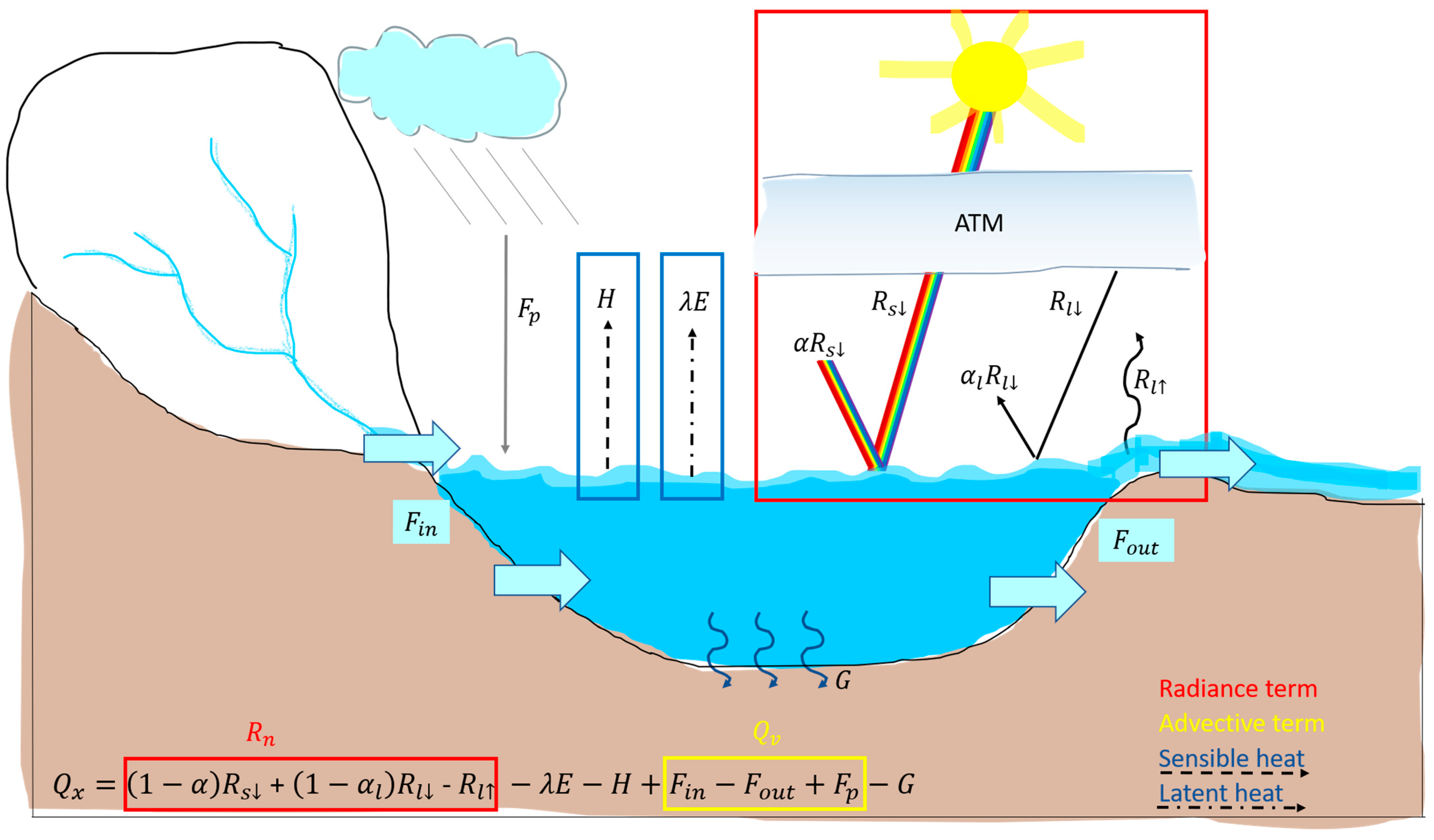
Figure 1. Representation of all terms of the heat balance in a water body.
Remotesensing 14 02636 g001
Figure 2. Workflow for the generation of evaporation products from LSWT maps.
Remotesensing 14 02636 g002
Figure 3. (a) Lake Garda study site and its location in Northern Italy; (b) location of the in-situ weather station MET1 and ERA5 and WRF models grid points. Filled orange diamonds and blue circles highlight the in-lake points from ERA5 and WRF grid points, respectively.
Remotesensing 14 02636 g003
Figure 4. Instantaneous evaporation ( E h ) maps for Lake Garda obtained from the year 2016 estimated with the LakeVap tool fed by CCI-Lakes LSWT maps and WRF (spatially averaged) meteorological data.
Remotesensing 14 02636 g004
Figure 5. (a) Comparison between instantaneous evaporation ( E h ) from Lake Garda, estimated with LakeVap using CCI-Lakes dataset and WRF spatially averaged meteorological data, and hourly evaporation simulated by Delft3D hydrodynamic model. (b) Comparison between LSWT derived from CCI-Lakes dataset and simulated by Delft3D hydrodynamic model. Shaded areas represent the standard deviation from the spatial mean (continuous line). To ease the comparison, the results from Delft3D are plotted on the days when LakeVap products are available (blue line), while the std (light blue shadow) is provided for all simulated days.
Remotesensing 14 02636 g005
Figure 6. (a) Instantaneous evaporation ( E h ) from Lake Garda estimated with LakeVap using CCI-Lakes dataset and different meteorological data sources. Lines depict the spatial average of E h maps obtained with meteo variables from ERA5 (orange continuous line), WRF (blue continuous line), and in-situ observations at MET1 (dashed green line) and MET2 (dotted magenta line) weather stations (see Figure 3b for the location of MET1 and MET2). The light-yellow shaded area represents the range of variation of E h due to different meteorological sources. (b) Scatterplots of air temperature, wind, and relative humidity as obtained from WRF (averaged over the lake surface), MET1, and MET2 in-situ data against ERA5 (averaged over the lake surface); (c) probability distribution of air temperature, wind, and relative humidity from the four datasets.
Remotesensing 14 02636 g006
Figure 7. (a) Mean spatial variation of LSWT and meteorological variables used to compute E h . The percentage of variation of each quantity is obtained as a time average of the spatial anomalies normalized by the mean (in time) fields as in Equation (7). (b) Mean spatial variation of E h obtained by feeding the LakeVap tool with all meteorological variables as uniform in space (first panel), with single variables spatialized (panels 2–4), variables spatialized pairwise (panels 5–7), and all variables spatialized (panel 8).
Remotesensing 14 02636 g007
Figure 8. Daily evaporation from Lake Garda estimated with the LakeVap tool fed by CCI-Lakes LSWT maps and ERA5 meteorological data (spatial average from daily evaporation maps). The gaps in the time series highlight when LSWT maps are not available for more than 60 consecutive days.
Remotesensing 14 02636 g008
Table 2. Summary of data used in this study from in-situ, remote sensing, and numerical modeling.
Type of DataTime AvailabilityIDData ProviderFrequencySpatial Resolution
LSWT maps1995–2019CCI-LakesESADaily to weekly100 m
In-situ weather data1990-dateMET1FEMHourlySingle point
2012-dateMET2ARPA-LombardiaHourlySingle point
Global model weather data1950-dateERA5ECMWFHourly0.1° (~11 km)
Regional model weather data2004–2018WRF[35,59]Hourly2 km
Simulated instantaneous evaporation maps2004–2018Delft3D[35]Daily100–400 m
Table 3. Performance of LakeVap tool based on CCI-Lakes LSWT and WRF, MET1, MET2, and ERA5 meteorological data. Metrics are computed for instantaneous evaporation estimates ( E h ) and for CCI-Lakes LSWT maps. Metrics assume Delft3D model results as the “true” value. * statistics computed on a shorter time series (2012–2018) due to the reduced availability of MET2 data.
Instantaneous Evaporation
Meteorology SourceRMSDBIASCorrNSEMean ± Std LakeVapMean ± Std Delft3D
(mm/h)(mm/h)(-)(-)(mm/h)(mm/h)
WRF0.040.0060.920.8340.129 ± 0.0810.128 ± 0.098
MET10.087−0.020.5170.2180.101 ± 0.058
MET2 *0.0810.0010.6140.3080.128 ± 0.0858
ERA50.091−0.0450.6060.1290.078 ± 0.044
Lake Surface Water Temperature
LSWT sourceRMSDBIASCorrNSEMean ± Std CCI-LakesMean ± Std Delft3D
(°C)(°C)(-)(-)(°C)(°C)
CCI-Lakes database1.7450.5360.9580.90614.81 ± 5.7514.27 ± 5.95
Publisher’s Note: MDPI stays neutral with regard to jurisdictional claims in published maps and institutional affiliations.