
Inversion of Ocean Subsurface Temperature and Salinity Fields Based on Spatio-Temporal Correlation


Abstract
1. Introduction
2. Study Area and Data
3. Methods
3.1. Random Forests
3.2. LSTM
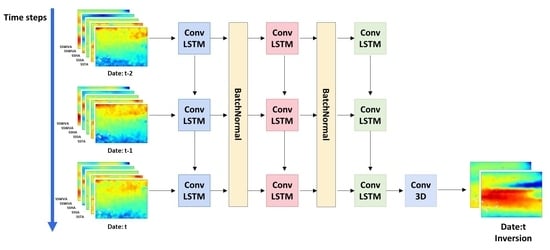
3.3. ConvLSTM
3.4. Experimental Setup
- -
- Hardware: Intel I9-11900K CPU, NVIDIA RTX 3090 GPU.
- -
- System environment: Ubuntu 18.04 system, Python 3.8.2, Tensorflow 2.4.0, Keras 2.4.3.
4. Results and Discussion
4.1. Comparison of Multiple Channels
4.2. Spatial Error Analysis
4.3. Temporal Error Analysis
4.4. Longitude Profile Validation
4.5. Comparison of Different Models
4.6. Comparison of Different Temporal and Spatial Scales
5. Conclusions
Supplementary Materials
Author Contributions
Funding
Data Availability Statement
Conflicts of Interest
References
- Bindoff, N.L.; Willebrand, J.; Artale, V.; Cazenave, A.; Gregory, J.M.; Gulev, S.; Hanawa, K.; Le Quere, C.; Levitus, S.; Nojiri, Y.; et al. Observations: Oceanic climate change and sea level. In Climate Change 2007: The Physical Science Basis; Cambridge University Press: Cambridge, UK, 2007. [Google Scholar]
- Meyssignac, B.; Boyer, T.; Zhao, Z.; Hakuba, M.Z.; Landerer, F.; Stammer, D.; Köhl, A.; Kato, S.; L’Ecuyer, T.; Ablain, M. Measuring Global Ocean Heat Content: To Estimate Earth’s Energy Imbalance. Front. Mar. Sci. 2019, 6, 437. [Google Scholar] [CrossRef]
- Johnson, G.C.; Lyman, J.M. Warming trends increasingly dominate global ocean. Nat. Clim. Chang. 2020, 10, 757–761. [Google Scholar] [CrossRef]
- Boyer, T.; Domingues, C.M.; Good, S.A.; Johnson, G.C.; Lyman, J.M.; Ishii, M.; Gouretski, V.; Willis, J.K.; Antonov, J.; Wijffels, S.; et al. Sensitivity of global upper-ocean heat content estimates to mapping methods, XBT bias corrections, and baseline climatologies. J. Clim. 2016, 29, 4817–4842. [Google Scholar] [CrossRef]
- Balmaseda, M.A.; Trenberth, K.E.; Källén, E. Distinctive climate signals in reanalysis of global ocean heat content. Geophys. Res. Lett. 2013, 40, 1754–1759. [Google Scholar] [CrossRef]
- Chen, X.; Tung, K.K. Varying planetary heat sink led to global-warming slowdown and acceleration. Science 2014, 345, 897–903. [Google Scholar] [CrossRef]
- Drijfhout, S.S.; Blaker, A.T.; Josey, S.A.; Nurser, A.J.; Sinha, B.; Balmaseda, M.A. Surface warming hiatus caused by increased heat uptake across multiple ocean basins. Geophys. Res. Lett. 2014, 41, 7868–7874. [Google Scholar] [CrossRef]
- Song, Y.T.; Colberg, F. Deep ocean warming assessed from altimeters, Gravity Recovery and Climate Experiment, in situ measurements, and a non-Boussinesq ocean general circulation model. J. Geophys. Res. Ocean. 2011, 116, C0202. [Google Scholar] [CrossRef]
- Bao, S.; Zhang, R.; Wang, H.; Yan, H.; Yu, Y.; Chen, J. Salinity profile estimation in the Pacific Ocean from satellite surface salinity observations. J. Atmos. Ocean. Technol. 2019, 36, 53–68. [Google Scholar] [CrossRef]
- Cazenave, A.; Meyssignac, B.; Ablain, M.; Balmaseda, M.; Bamber, J.; Barletta, V.; Beckley, B.; Benveniste, J.; Berthier, E.; Blazquez, A.; et al. Global sea-level budget 1993-present. Earth Syst. Sci. Data 2018, 10, 1551–1590. [Google Scholar]
- Lu, W.; Su, H.; Yang, X.; Yan, X.H. Subsurface temperature estimation from remote sensing data using a clustering-neural network method. Remote Sens. Environ. 2019, 229, 213–222. [Google Scholar] [CrossRef]
- Su, H.; Wu, X.; Lu, W.; Zhang, W.; Yan, X.H. Inconsistent Subsurface and Deeper Ocean Warming Signals During Recent Global Warming and Hiatus. J. Geophys. Res. Ocean. 2017, 122, 8182–8195. [Google Scholar] [CrossRef]
- Wang, G.; Cheng, L.; Abraham, J.; Li, C. Consensuses and discrepancies of basin-scale ocean heat content changes in different ocean analyses. Clim. Dyn. 2018, 50, 2471–2487. [Google Scholar] [CrossRef]
- Jayne, S.R.; Roemmich, D.; Zilberman, N.; Riser, S.C.; Johnson, K.S.; Johnson, G.C.; Piotrowicz, S.R. The argo program: Present and future. Oceanography 2017, 30, 18–28. [Google Scholar] [CrossRef]
- Su, H.; Wu, X.; Yan, X.H.; Kidwell, A. Estimation of subsurface temperature anomaly in the Indian Ocean during recent global surface warming hiatus from satellite measurements: A support vector machine approach. Remote Sens. Environ. 2015, 160, 63–71. [Google Scholar] [CrossRef]
- Su, H.; Huang, L.; Li, W.; Yang, X.; Yan, X.H. Retrieving Ocean Subsurface Temperature Using a Satellite-Based Geographically Weighted Regression Model. J. Geophys. Res. Ocean. 2018, 123, 5180–5193. [Google Scholar] [CrossRef]
- Guinehut, S.; Dhomps, A.L.; Larnicol, G.; Le Traon, P.Y. High resolution 3-D temperature and salinity fields derived from in situ and satellite observations. Ocean. Sci. 2012, 8, 845–857. [Google Scholar] [CrossRef]
- Liu, L.; Peng, S.; Wang, J.; Huang, R.X. Retrieving density and velocity fields of the ocean’s interior from surface data. J. Geophys. Res. Ocean. 2014, 119, 8512–8529. [Google Scholar] [CrossRef]
- Liu, L.E.; Xue, H.; Sasaki, H. Reconstructing the Ocean Interior from High-Resolution Sea Surface Information. J. Phys. Oceanogr. 2019, 49, 3245–3262. [Google Scholar] [CrossRef]
- Wang, J.; Flierl, G.R.; Lacasce, J.H.; Mcclean, J.L.; Mahadevan, A. Reconstructing the Ocean’s Interior from Surface Data. J. Phys. Oceanogr. 2013, 43, 1611–1626. [Google Scholar] [CrossRef]
- Yan, X.H.; Jo, Y.H.; Liu, W.T.; He, M.X. A New Study of the Mediterranean Outflow, Air–Sea Interactions, and Meddies Using Multisensor Data. J. Phys. Oceanogr. 2006, 36, 691–710. [Google Scholar] [CrossRef][Green Version]
- Yan, X.-H.; Okubo, A. Three-dimensional analytical model for the mixed layer depth. J. Geophys. Res. Ocean. 1992, 97, 20201–20226. [Google Scholar] [CrossRef]
- Akbari, E.; Alavipanah, S.K.; Jeihouni, M.; Hajeb, M.; Haase, D.; Alavipanah, S. A Review of Ocean/Sea Subsurface Water Temperature Studies from Remote Sensing and Non-Remote Sensing Methods. Water 2017, 9, 936. [Google Scholar] [CrossRef]
- Holloway, J.; Mengersen, K. Statistical Machine Learning Methods and Remote Sensing for Sustainable Development Goals: A Review. Remote Sens. 2018, 10, 1365. [Google Scholar] [CrossRef]
- Klemas, V.; Yan, X.H. Subsurface and deeper ocean remote sensing from satellites: An overview and new results. Prog. Oceanogr. 2014, 122, 1–9. [Google Scholar] [CrossRef]
- Lary, D.J.; Alavi, A.H.; Gandomi, A.H.; Walker, A.L. Machine learning in geosciences and remote sensing. Geosci. Front. 2016, 7, 3–10. [Google Scholar] [CrossRef]
- Carnes, M.R.; Teague, W.J.; Mitchell, J. Inference of subsurface thermohaline structure from fields measurable by satellite. J. Atmos. Ocean. Technol. 1994, 11, 2. [Google Scholar] [CrossRef]
- Fox, D.; Teague, W.; Barron, C.; Carnes, M.; Lee, C. The modular ocean data assimilation system (MODAS). J. Atmos. Ocean. Technol. 2002, 19, 240–252. [Google Scholar] [CrossRef]
- Nardelli, B.; Santoleri, R. Reconstructing synthetic profiles from surface data. J. Atmos. Ocean. Technol. 2004, 21, 693–703. [Google Scholar] [CrossRef]
- Jeong, Y.; Hwang, J.; Park, J.; Jang, C.J.; Jo, Y.H. Reconstructed 3-D Ocean Temperature Derived from Remotely Sensed Sea Surface Measurements for Mixed Layer Depth Analysis. Remote Sens. 2019, 11, 3018. [Google Scholar] [CrossRef]
- Maes, C.; Behringer, D.; Reynolds, R.W.; Ming, J. Retrospective analysis of the salinity variability in the western tropical Pacific Ocean using an indirect minimization approach. J. Atmos. Ocean. Technol. 2000, 17, 512–524. [Google Scholar] [CrossRef]
- Nardelli, B.B.; Santoleri, R. Methods for the Reconstruction of Vertical Profiles from Surface Data: Multivariate Analyses, Residual GEM, and Variable Temporal Signals in the North Pacific Ocean. J. Atmos. Ocean. Technol. 2005, 22, 1762–1781. [Google Scholar] [CrossRef]
- Ali, M.; Swain, D.; Weller, R. Estimation of ocean subsurface thermal structure from surface parameters: A neural network approach. Geophys. Res. Lett. 2004, 31, L20308. [Google Scholar] [CrossRef]
- Su, H.; Zhang, H.; Geng, X.; Qin, T.; Lu, W.; Yan, X.H. OPEN: A new estimation of global ocean heat content for upper 2000 meters from remote sensing data. Remote Sens. 2020, 12, 2294. [Google Scholar] [CrossRef]
- Wu, X.; Yan, X.H.; Jo, Y.H.; Liu, W.T. Estimation of Subsurface Temperature Anomaly in the North Atlantic Using a Self-Organizing Map Neural Network. J. Atmos. Ocean. Technol. 2012, 29, 1675–1688. [Google Scholar] [CrossRef]
- Chapman, C.; Charantonis, A.A. Reconstruction of Subsurface Velocities from Satellite Observations Using Iterative Self-Organizing Maps. IEEE Geosci. Remote Sens. Lett. 2017, 14, 617–620. [Google Scholar] [CrossRef]
- Chen, C.; Yang, K.; Ma, Y.; Wang, Y. Reconstructing the Subsurface Temperature Field by Using Sea Surface Data Through Self-Organizing Map Method. IEEE Geosci. Remote Sens. Lett. 2018, 15, 1812–1816. [Google Scholar] [CrossRef]
- Su, H.; Li, W.; Yan, X.H. Retrieving Temperature Anomaly in the Global Subsurface and Deeper Ocean from Satellite Observations. J. Geophys. Res. Ocean. 2018, 123, 399–410. [Google Scholar] [CrossRef]
- Su, H.; Yang, X.; Lu, W.; Yan, X.H. Estimating subsurface thermohaline structure of the global ocean using surface remote sensing observations. Remote Sens. 2019, 11, 1598. [Google Scholar] [CrossRef]
- Goodfellow, I.; Bengio, Y.; Courville, A. Deep Learning; MIT Press: Cambridge, MA, USA, 2016. [Google Scholar]
- Bolton, T.; Zanna, L. Applications of Deep Learning to Ocean Data Inference and Subgrid Parameterization. J. Adv. Model. Earth Syst. 2019, 11, 376–399. [Google Scholar] [CrossRef]
- Ham, Y.G.; Kim, J.H.; Luo, J.J. Deep learning for multi-year ENSO forecasts. Nature 2019, 573, 568–572. [Google Scholar] [CrossRef]
- Song, T.; Jiang, J.; Li, W.; Xu, D. A Deep Learning Method with Merged LSTM Neural Networks for SSHA Prediction. IEEE J. Sel. Top. Appl. Earth Obs. Remote Sens. 2020, 13, 2853–2860. [Google Scholar] [CrossRef]
- Song, T.; Li, Y.; Meng, F.; Xie, P.; Xu, D. A Novel Deep Learning Model by BiGRU with Attention Mechanism for Tropical Cyclone Track Prediction in Northwest Pacific. J. Appl. Meteorol. Climatol. 2021, 61, 3–12. [Google Scholar] [CrossRef]
- Song, T.; Wang, J.; Xu, D.; Wei, W.; Han, R.; Meng, F.; Li, Y. Unsupervised Machine Learning for Improved Delaunay Triangulation. J. Mar. Sci. Eng. 2021, 9, 1398. [Google Scholar] [CrossRef]
- Song, T.; Han, N.; Zhu, Y.; Li, Z.; Li, Y.; Li, S.; Peng, S. Application of deep learning technique to the sea surface height prediction in the South China Sea. Acta Oceanol. Sin. 2021, 40, 68–76. [Google Scholar] [CrossRef]
- Meng, F.; Song, T.; Xu, D.; Xie, P.; Li, Y. Forecasting tropical cyclones wave height using bidirectional gated recurrent unit. Ocean. Eng. 2021, 234, 108795. [Google Scholar] [CrossRef]
- Meng, F.; Xu, D.; Song, T. ATDNNS: An adaptive time–frequency decomposition neural network-based system for tropical cyclone wave height real-time forecasting. Future Gener. Comput. Syst. 2022, 133, 297–306. [Google Scholar] [CrossRef]
- Meng, F.; Song, T.; Xu, D. Simulating Tropical Cyclone Passive Microwave Rainfall Imagery Using Infrared Imagery via Generative Adversarial Networks. IEEE Geosci. Remote Sens. Lett. 2022, 19, 1–5. [Google Scholar] [CrossRef]
- Uitz, J.; Claustre, H.; Morel, A.; Hooker, S.B. Vertical distribution of phytoplankton communities in open ocean: An assessment based on surface chlorophyll. J. Geophys. Res. Ocean. 2006, 111, C08005. [Google Scholar] [CrossRef]
- Charantonis, A.A.; Badran, F.; Thiria, S. Retrieving the evolution of vertical profiles of Chlorophyll-a from satellite observations using Hidden Markov Models and Self-Organizing Topological Maps. Remote Sens. Environ. 2015, 163, 229–239. [Google Scholar] [CrossRef]
- Hochreiter, S.; Schmidhuber, J. Long short-term memory. Neural Comput. 1997, 9, 1735–1780. [Google Scholar] [CrossRef]
- Shi, X.; Chen, Z.; Wang, H.; Yeung, D.Y.; Wong, W.K.; Woo, W. Convolutional LSTM network: A machine learning approach for precipitation nowcasting. In Proceedings of the 29th Annual Conference on Neural Information Processing Systems, Montreal, QC, Canada, 7–12 December 2015. [Google Scholar]
- Li, H.; Xu, F.; Zhou, W.; Wang, D.; Wright, J.S.; Liu, Z.; Lin, Y. Development of a global gridded A rgo data set with B arnes successive corrections. J. Geophys. Res. Ocean. 2017, 122, 866–889. [Google Scholar] [CrossRef]
- Huang, B.; Liu, C.; Banzon, V.; Freeman, E.; Graham, G.; Hankins, B.; Smith, T.; Zhang, H.M. Improvements of the daily optimum interpolation sea surface temperature (DOISST) version 2.1. J. Clim. 2021, 34, 2923–2939. [Google Scholar] [CrossRef]
- Kerr, Y.H.; Waldteufel, P.; Wigneron, J.P.; Delwart, S.; Cabot, F.; Boutin, J.; Escorihuela, M.J.; Font, J.; Reul, N.; Gruhier, C.; et al. The SMOS mission: New tool for monitoring key elements ofthe global water cycle. Proc. IEEE 2010, 98, 666–687. [Google Scholar] [CrossRef]
- Hauser, D.; Tourain, C.; Hermozo, L.; Alraddawi, D.; Aouf, L.; Chapron, B.; Dalphinet, A.; Delaye, L.; Dalila, M.; Dormy, E.; et al. New observations from the SWIM radar on-board CFOSAT: Instrument validation and ocean wave measurement assessment. IEEE Trans. Geosci. Remote Sens. 2020, 59, 5–26. [Google Scholar] [CrossRef]
- Atlas, R.; Hoffman, R.N.; Ardizzone, J.; Leidner, S.M.; Jusem, J.C.; Smith, D.K.; Gombos, D. A cross-calibrated, multiplatform ocean surface wind velocity product for meteorological and oceanographic applications. Bull. Am. Meteorol. Soc. 2011, 92, 157–174. [Google Scholar] [CrossRef]
- Chassignet, E.P.; Hurlburt, H.E.; Smedstad, O.M.; Halliwell, G.R.; Hogan, P.J.; Wallcraft, A.J.; Baraille, R.; Bleck, R. The HYCOM (hybrid coordinate ocean model) data assimilative system. J. Mar. Syst. 2007, 65, 60–83. [Google Scholar] [CrossRef]
- Breiman, L. Random forests. Mach. Learn. 2001, 45, 5–32. [Google Scholar] [CrossRef]
- Su, H.; Qin, T.; Wang, A.; Lu, W. Reconstructing ocean heat content for revisiting global ocean warming from remote sensing perspectives. Remote Sens. 2021, 13, 3799. [Google Scholar] [CrossRef]
- Graves, A. Generating sequences with recurrent neural networks. arXiv 2013, arXiv:1308.0850. [Google Scholar]


| Hyperparamaters | Meaning (Default) | Optimal Values |
|---|---|---|
| num_layers_ConvLSTM | The layer of the ConvLSTM model | 3 |
| num_units_ConvLSTM | The number of neurons in each ConvLSTM layer | 3 |
| kernel_size_ConvLSTM | The size of the convolution kernel in ConvLSTM layer | 8 × 8 |
| activation_ConvLSTM | The activation function used by ConvLSTM layer | Tanh |
| num_layers_Conv2D | The number of neurons in each ConvLSTM layer | 1 |
| kernel_size_Conv2D | The size of the convolution kernel in convolution layer | 5 × 5 |
| activation_Conv2D | The activation function used by Conv2D layer | Sigmod |
| time_step | The number of moments in each sample | Customized |
| batch_size | The number of sample input into the model each time | 32 |
| training_epoch | The number of epochs required for model training | 100 |
| early_stopping | The number of patience epochs required for early stopping | 10 |
| Case | Training Methods |
|---|---|
| Case 1A | ST_monthly = ConvLSTM (SSTA, SSSA, SSHA) |
| Case 2A | ST_monthly = ConvLSTM (SSTA, SSSA, SSHA, USSWA) |
| Case 3A | ST_monthly = ConvLSTM (SSTA, SSSA, SSHA, VSSWA) |
| Case 4A | ST_monthly = ConvLSTM (SSTA, SSSA, SSHA, USSWA, VSSWA) |
| Case 1B | SS_monthly = ConvLSTM (SSTA, SSSA, SSHA) |
| Case 2B | SS_monthly = ConvLSTM (SSTA, SSSA, SSHA, USSWA) |
| Case 3B | SS_monthly = ConvLSTM (SSTA, SSSA, SSHA, VSSWA) |
| Case 4B | SS_monthly = ConvLSTM (SSTA, SSSA, SSHA, USSWA, VSSWA) |
| Case RFs_A | ST_monthly = RFs (SSTA, SSSA, SSHA, USSWA, VSSWA) |
| Case RFs_B | SS_monthly = RFs (SSTA, SSSA, SSHA, USSWA, VSSWA) |
| Case LSTM_A | ST_monthly = LSTM (SSTA, SSSA, SSHA, USSWA, VSSWA) |
| Case LSTM_B | SS_monthly = LSTM (SSTA, SSSA, SSHA, USSWA, VSSWA) |
| Case 5A | ST_daily = ConvLSTM (SSTA, SSSA, SSHA) |
| Case 5B | SS_daily = ConvLSTM (SSTA, SSSA, SSHA) |
Publisher’s Note: MDPI stays neutral with regard to jurisdictional claims in published maps and institutional affiliations. |
© 2022 by the authors. Licensee MDPI, Basel, Switzerland. This article is an open access article distributed under the terms and conditions of the Creative Commons Attribution (CC BY) license (https://creativecommons.org/licenses/by/4.0/).
Share and Cite
Song, T.; Wei, W.; Meng, F.; Wang, J.; Han, R.; Xu, D. Inversion of Ocean Subsurface Temperature and Salinity Fields Based on Spatio-Temporal Correlation. Remote Sens. 2022, 14, 2587. https://doi.org/10.3390/rs14112587
Song T, Wei W, Meng F, Wang J, Han R, Xu D. Inversion of Ocean Subsurface Temperature and Salinity Fields Based on Spatio-Temporal Correlation. Remote Sensing. 2022; 14(11):2587. https://doi.org/10.3390/rs14112587
Chicago/Turabian StyleSong, Tao, Wei Wei, Fan Meng, Jiarong Wang, Runsheng Han, and Danya Xu. 2022. "Inversion of Ocean Subsurface Temperature and Salinity Fields Based on Spatio-Temporal Correlation" Remote Sensing 14, no. 11: 2587. https://doi.org/10.3390/rs14112587
APA StyleSong, T., Wei, W., Meng, F., Wang, J., Han, R., & Xu, D. (2022). Inversion of Ocean Subsurface Temperature and Salinity Fields Based on Spatio-Temporal Correlation. Remote Sensing, 14(11), 2587. https://doi.org/10.3390/rs14112587