
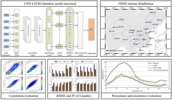
An Ionospheric TEC Forecasting Model Based on a CNN-LSTM-Attention Mechanism Neural Network


Abstract
:
1. Introduction
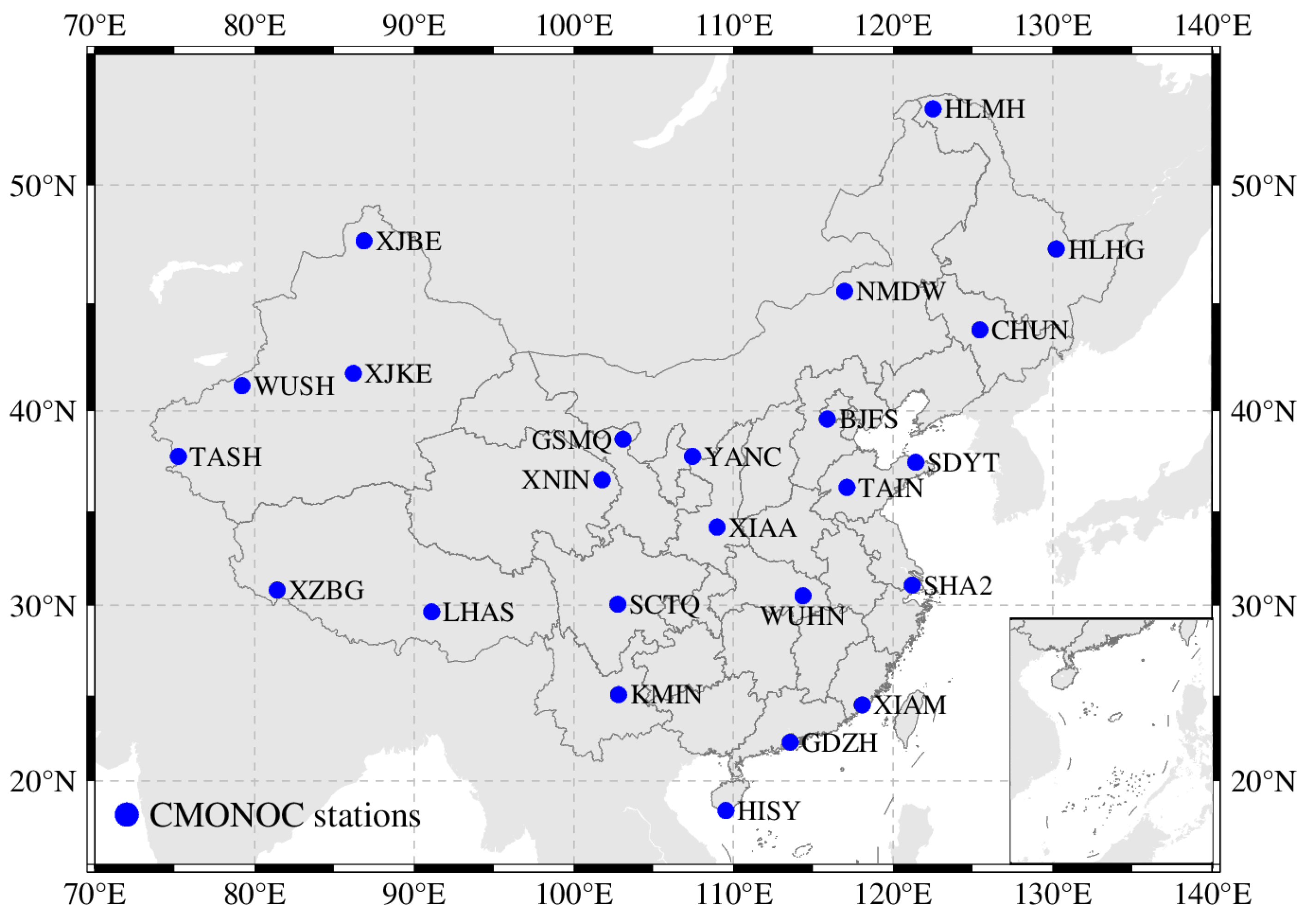
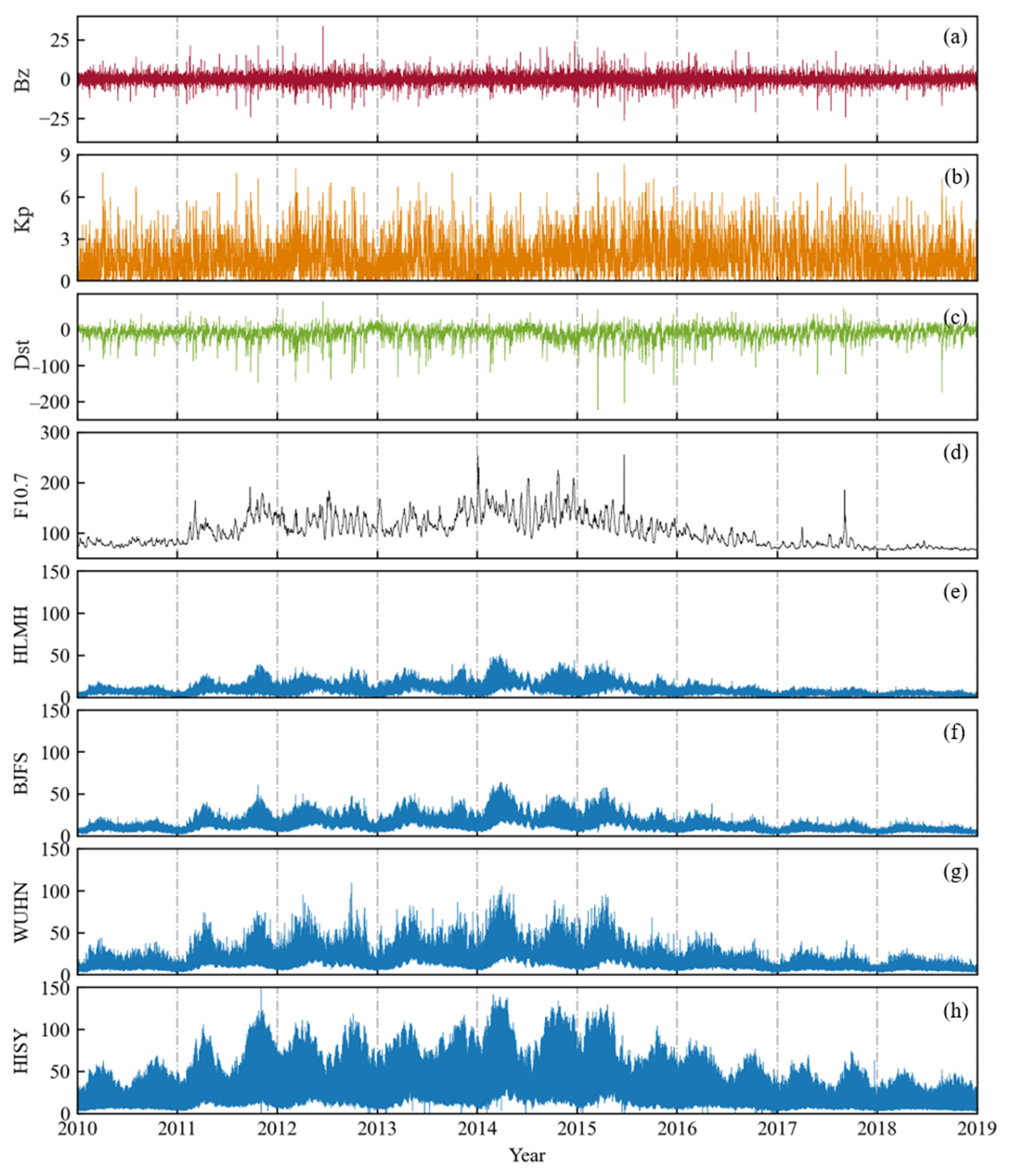
2. Data
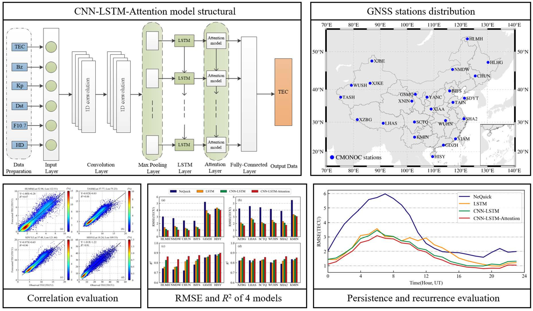
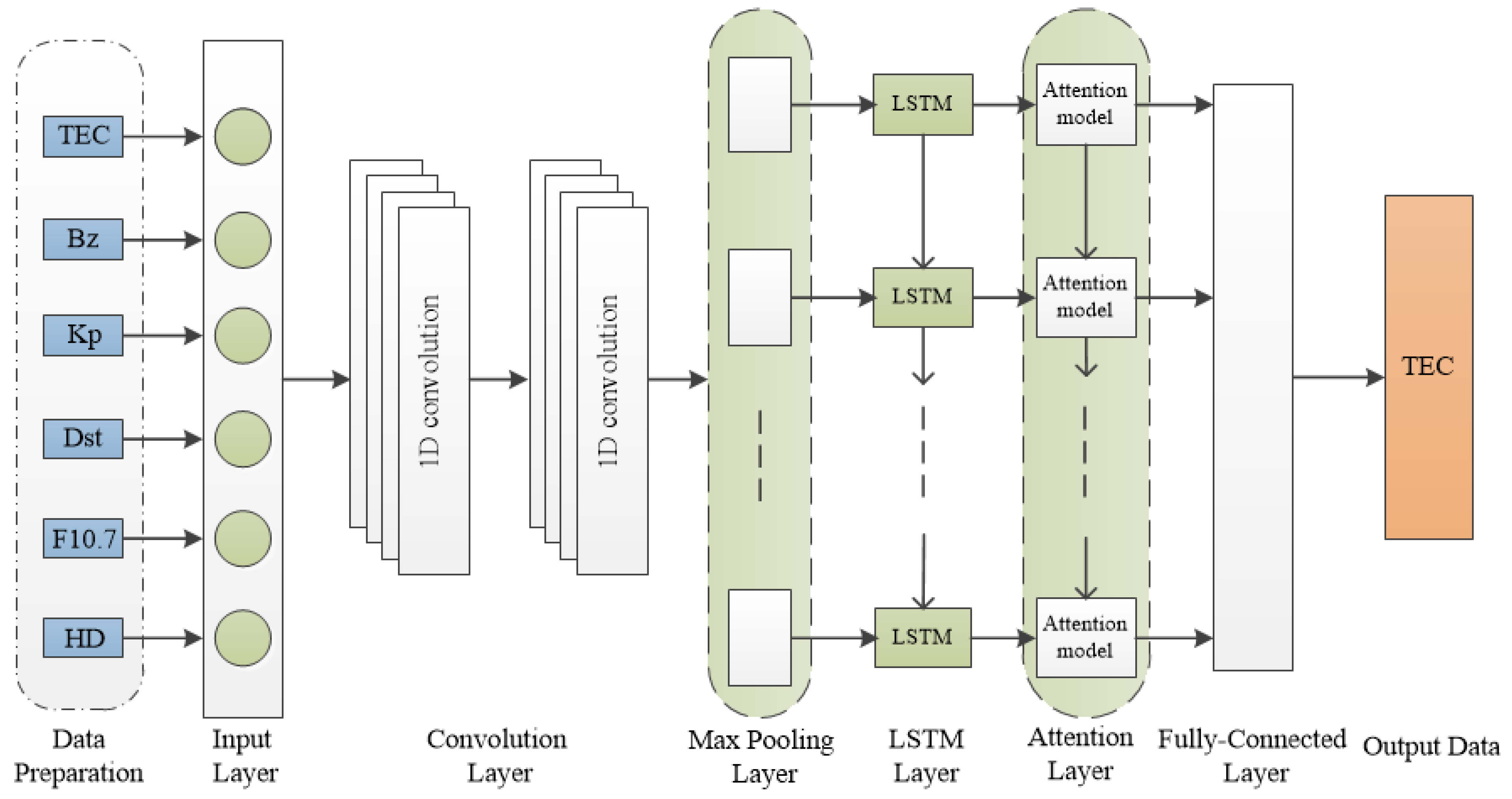
3. Model and Methodology
3.1. Convolutional Neural Network
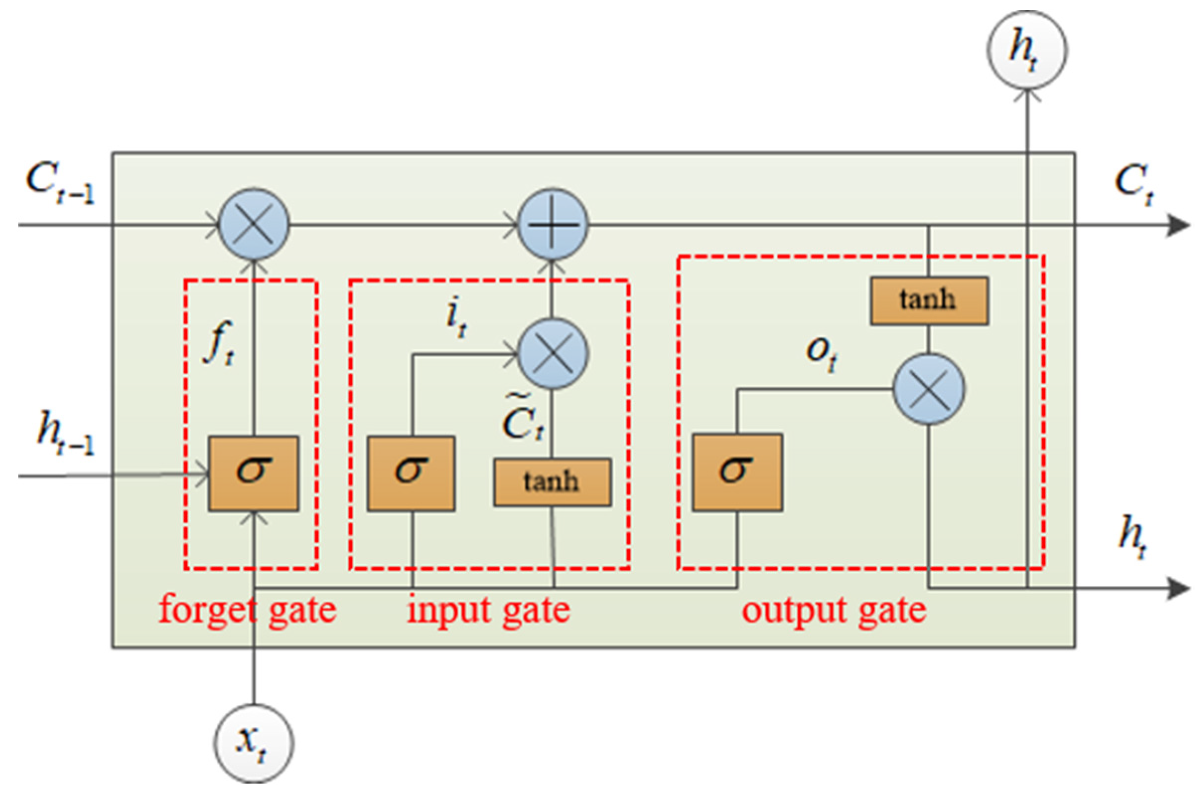
3.2. Long-Short Term Memory Neural Network
3.3. Attention Mechanism
3.4. Data Organization and Parameter Setting
4. Results and Evaluation
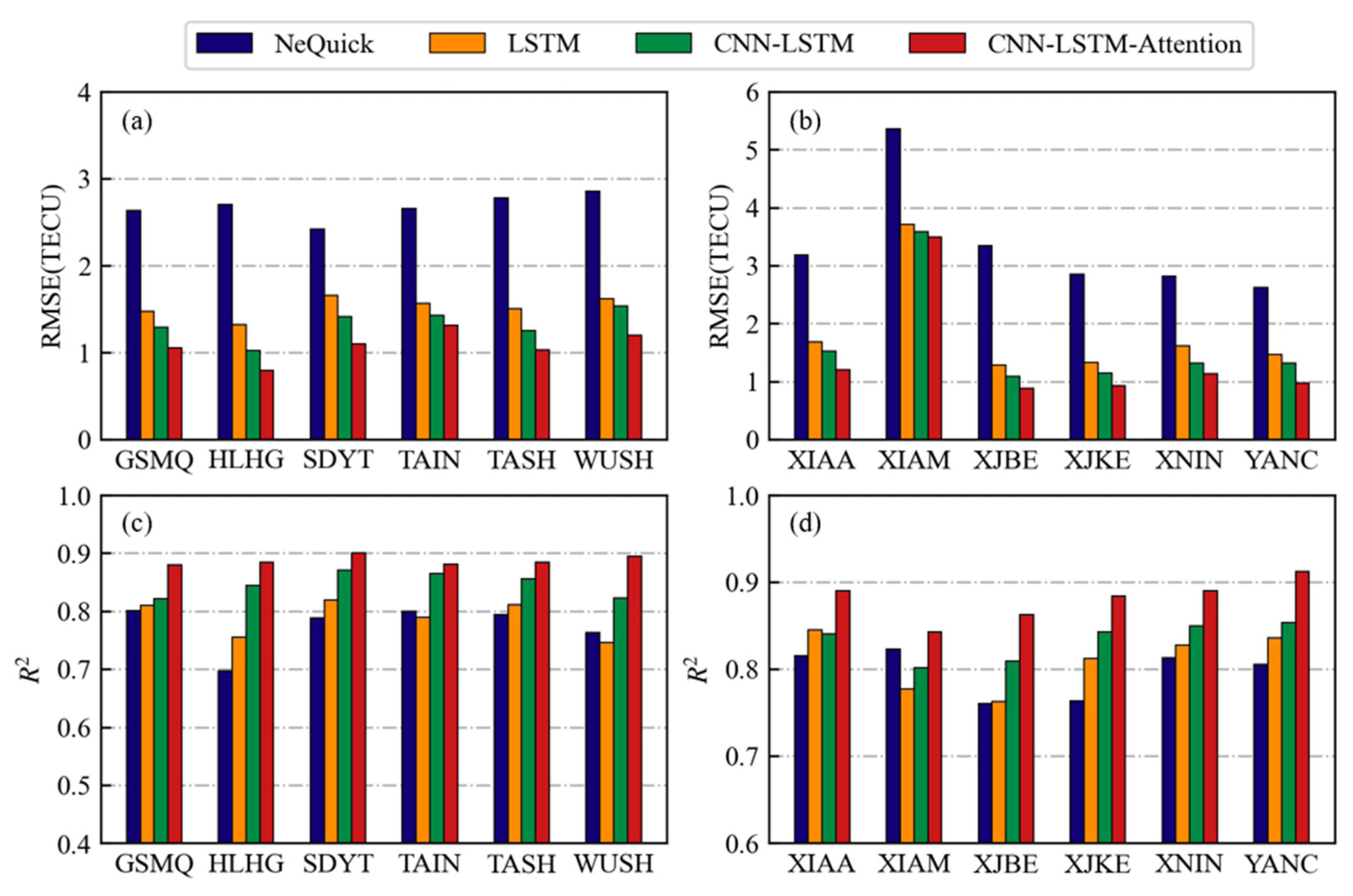
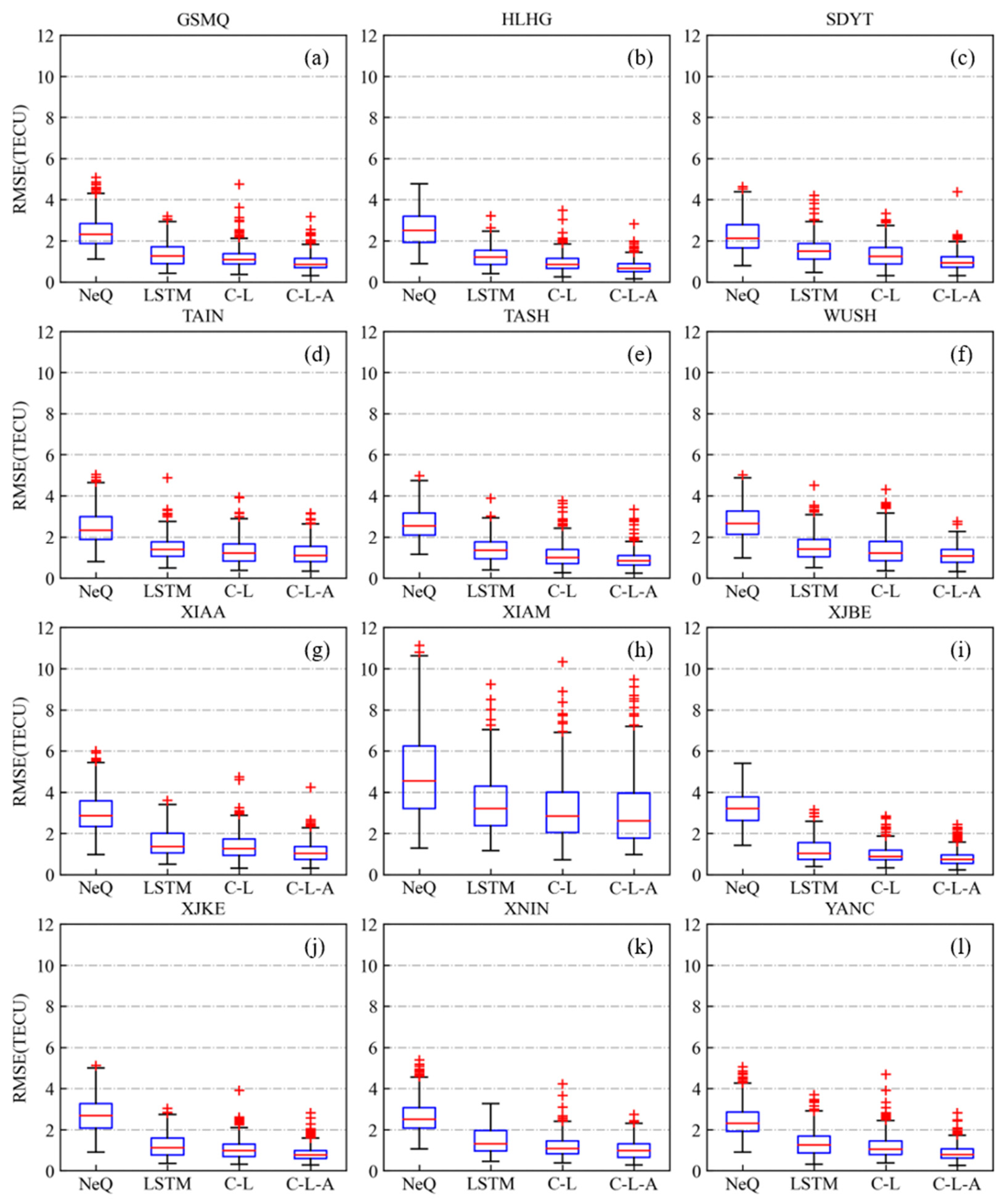
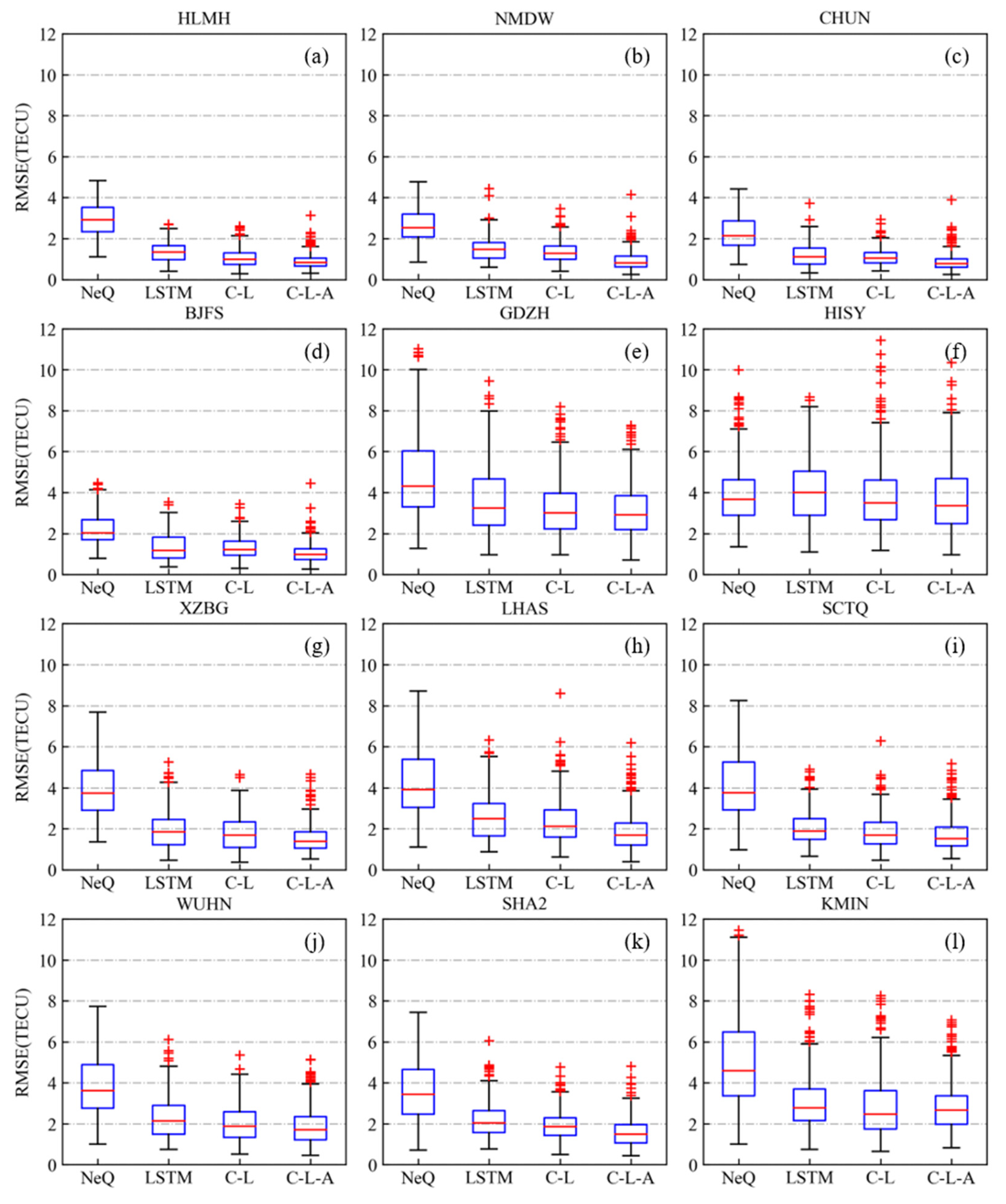
4.1. Accuracy Assessment of Different Stations
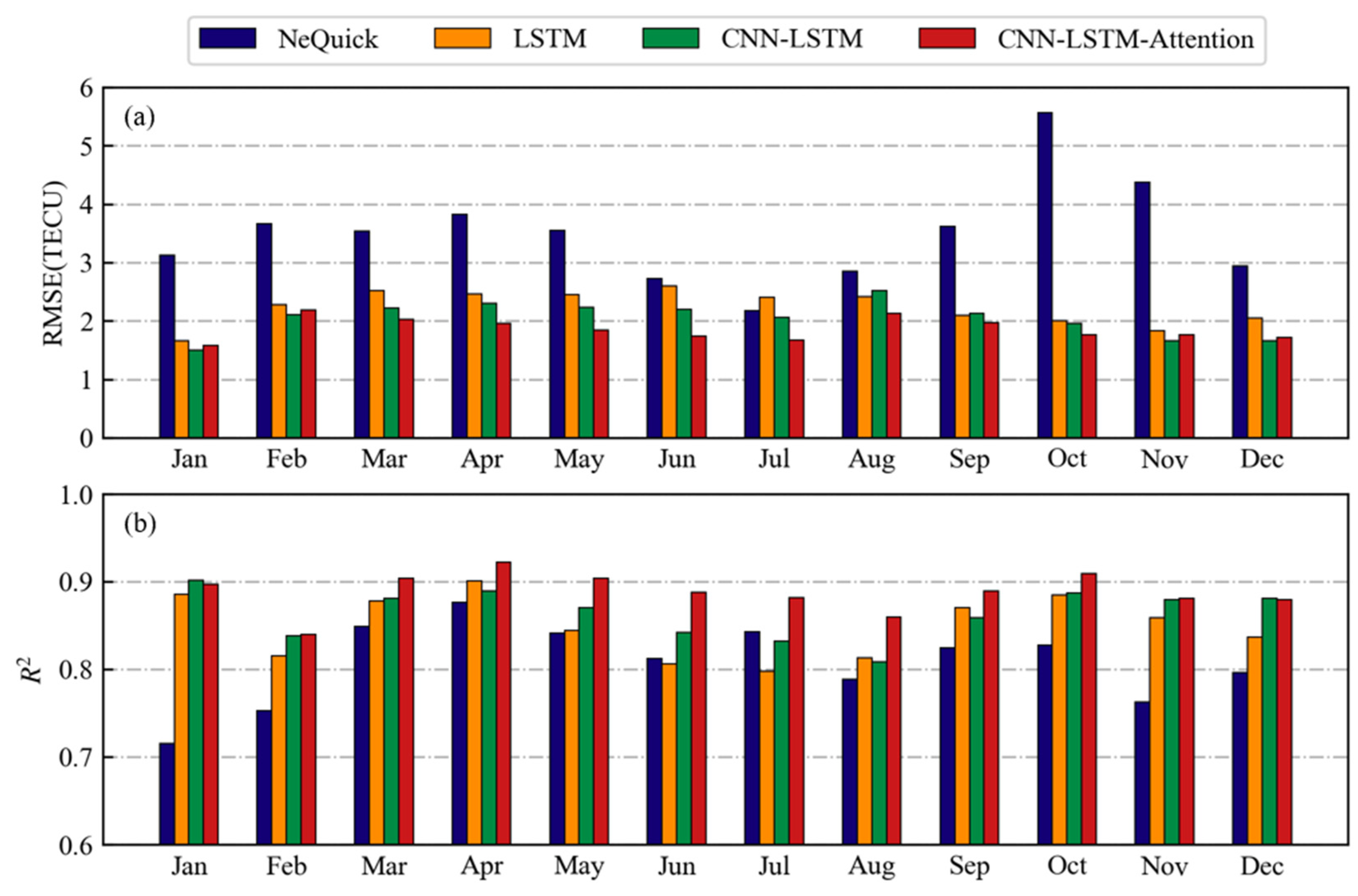
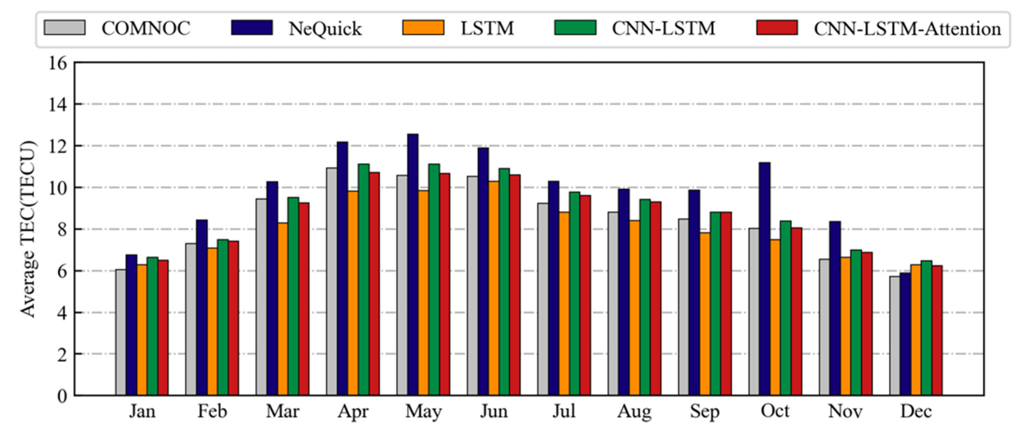
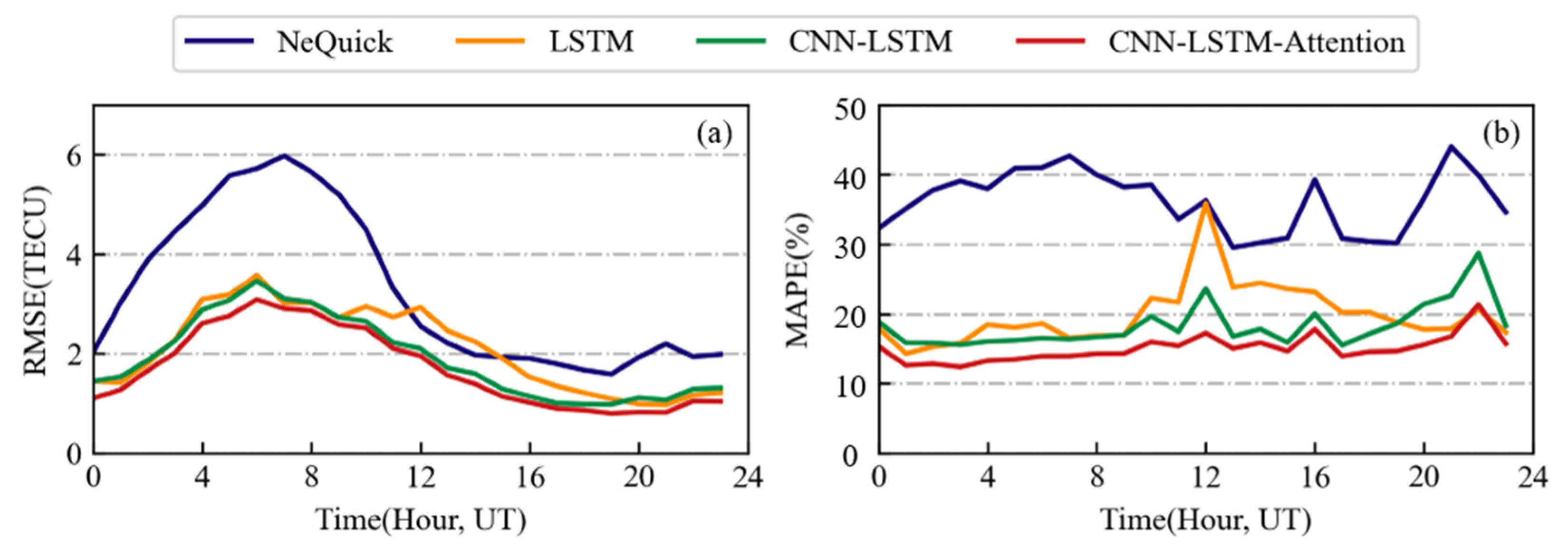
4.2. Accuracy Assessment at Different Time Periods
4.3. Accuracy Assessment under Different Geomagnetic Conditions
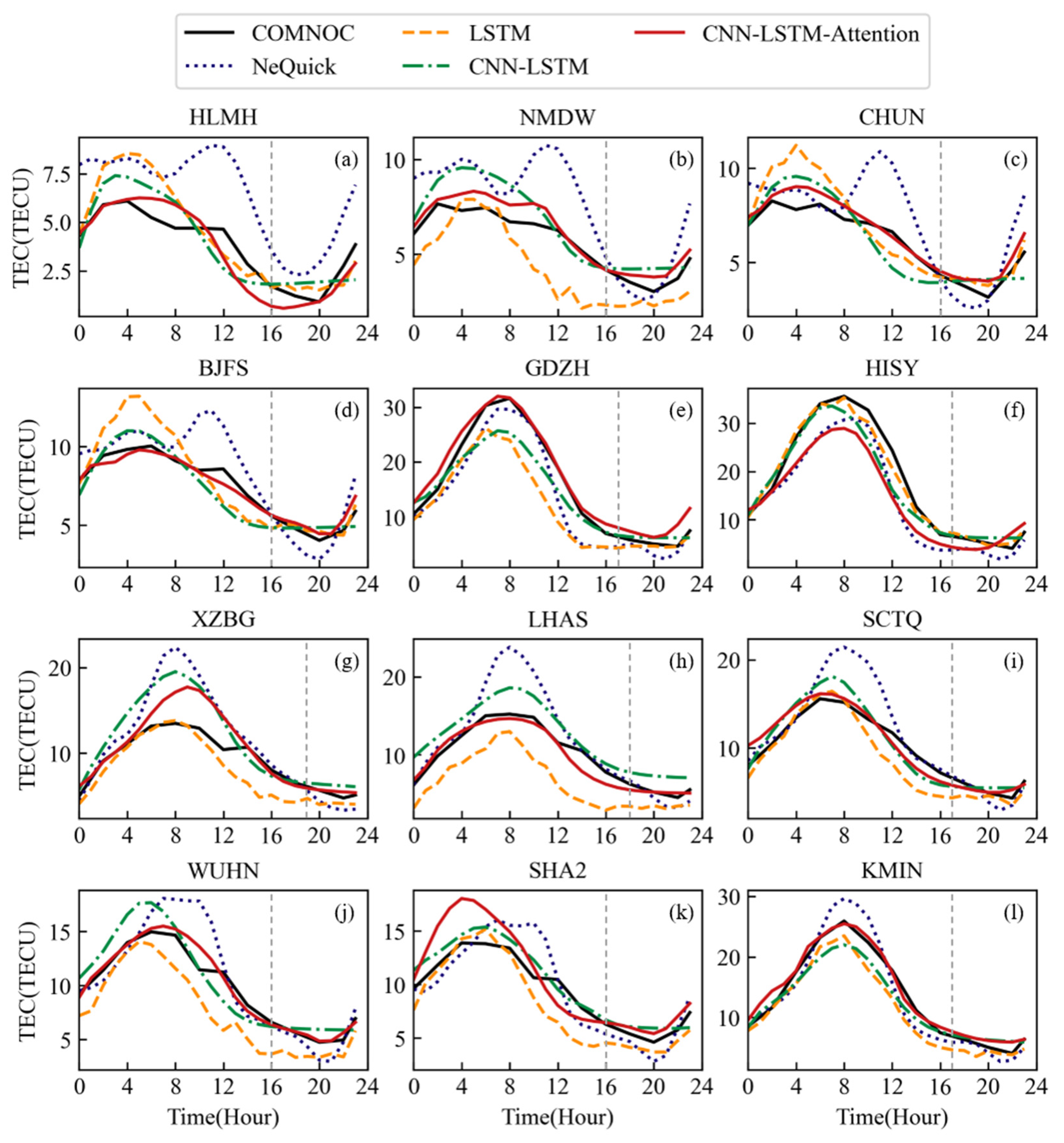
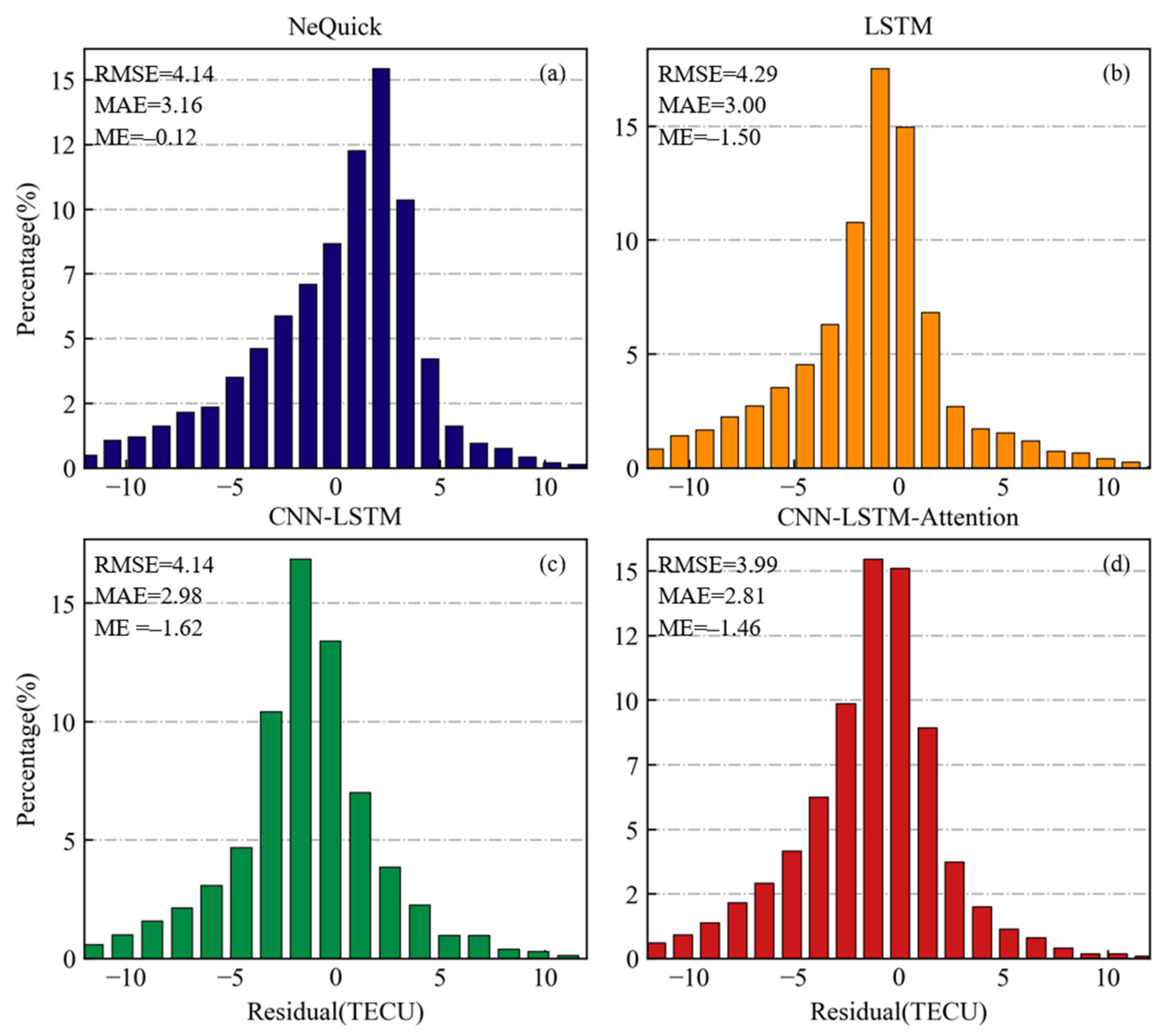
4.3.1. Magnetic Quiet Period
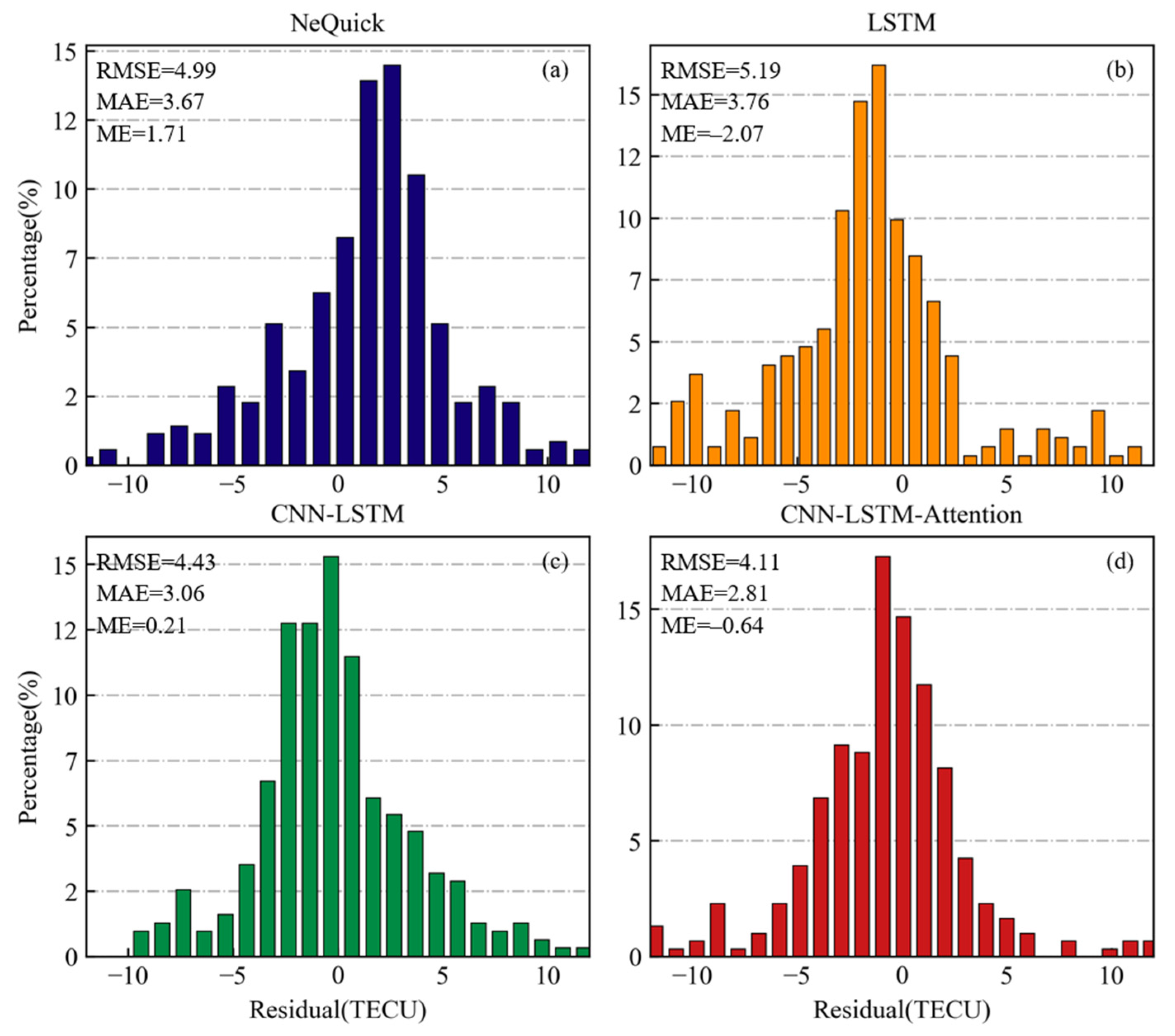
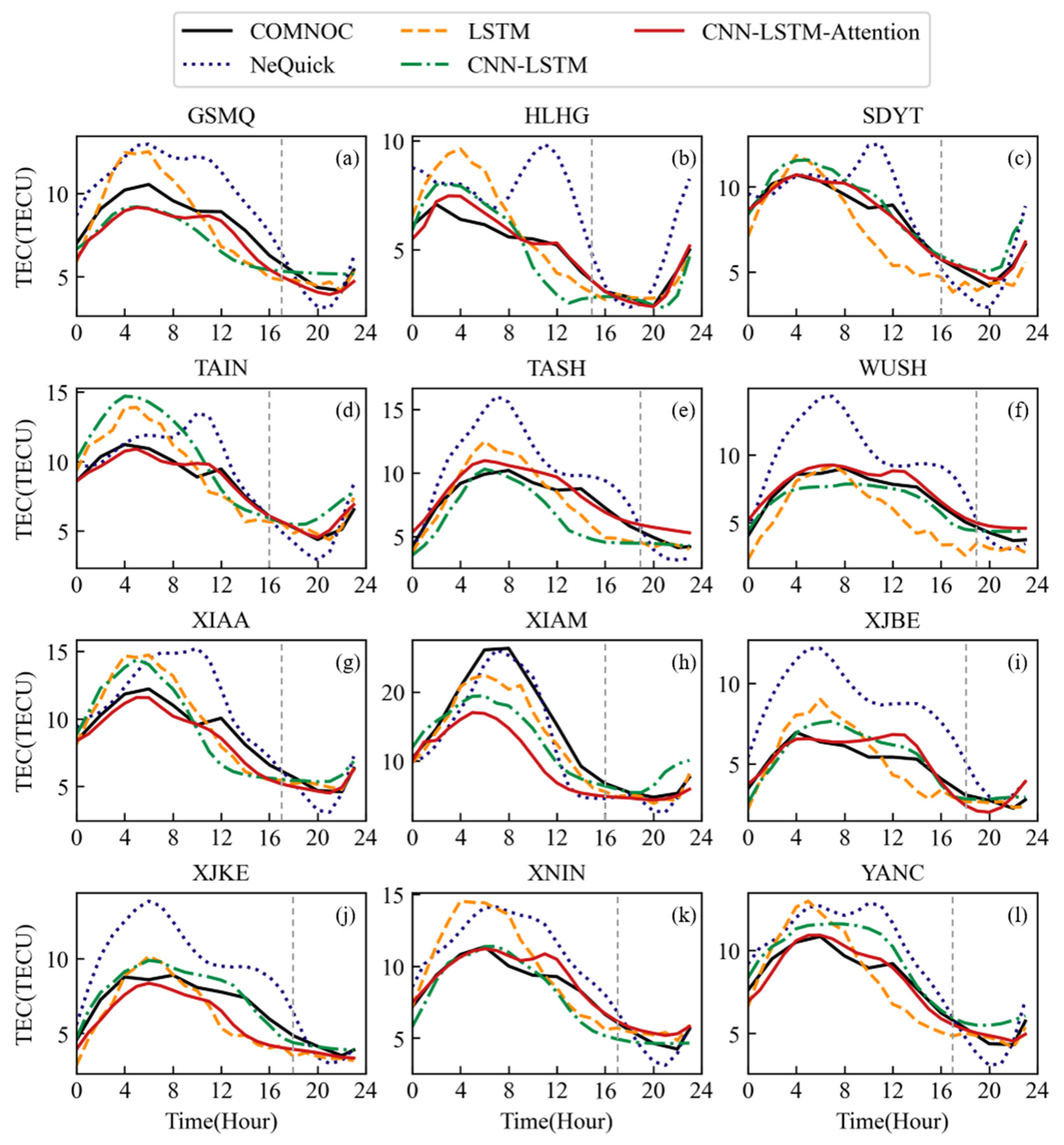
4.3.2. Magnetic Storm Period
5. Discussion
6. Conclusions
Author Contributions
Funding
Data Availability Statement
Acknowledgments
Conflicts of Interest
Appendix A


References
- Themens, D.R.; Reid, B.; Jayachandran, P.T.; Larson, B.; Koustov, A.V.; Elvidge, S.; McCaffrey, A.M.; Watson, C. E-CHAIM as a model of total electron content: Performance and diagnostics. Space Weather 2021, 19, e2021SW002872. [Google Scholar] [CrossRef]
- Francis, N.M.; Cannon, P.S.; Brown, A.G.; Broomhead, D.S. Nonlinear prediction of the ionospheric parameter foF2 on hourly, daily, and monthly timescales. J. Geophys. Res. 2000, 105, 12839–12849. [Google Scholar] [CrossRef]
- Francis, N.M.; Brown, A.G.; Cannon, P.S.; Broomhead, D.S. Prediction of the hourly ionospheric parameter foF2 using a novel nonlinear interpolation technique to cope with missing data points. J. Geophys. Res. 2001, 106, 30077–30083. [Google Scholar] [CrossRef]
- Tulunay, E.; Senalp, E.T.; Radicella, S.M.; Tulunay, Y. Forecasting total electron content maps by neural network technique. Radio Sci. 2006, 41, RS4016. [Google Scholar] [CrossRef]
- Habarulema, J.B.; McKinnell, L.A.; Opperman, B.D. Towards a GPS-based TEC prediction model for Southern Africa with feed forward networks. Adv. Space Res. 2009, 44, 82–92. [Google Scholar] [CrossRef]
- Habarulema, J.B.; McKinnell, L.-A.; Opperman, B.D.L. Regional GPS TEC modeling; Attempted spatial and temporal extrapolation of TEC using neural networks. J. Geophys. Res. 2011, 116, A04314. [Google Scholar] [CrossRef]
- Huang, L.; Wang, J.; Jiang, Y.; Huang, J.; Chen, Z.; Zhao, K. A preliminary study of the single crest phenomenon in total electron content (TEC) in the equatorial anomaly region around 120°E longitude between 1999 and 2012. Adv. Space Res. 2014, 54, 2200–2207. [Google Scholar] [CrossRef] [Green Version]
- Ferreira, A.A.; Borges, R.A.; Paparini, C.; Ciraolo, L.; Radicella, S.M. Short-term estimation of GNSS TEC using a neural network model in Brazil. Adv. Space Res. 2017, 60, 1765–1776. [Google Scholar] [CrossRef]
- Bai, H.; Fu, H.; Wang, J.; Ma, K.; Wu, T.; Ma, J. A prediction model of ionospheric foF2 based on extreme learning machine. Radio Sci. 2018, 53, 1292–1301. [Google Scholar] [CrossRef]
- Lee, S.; Ji, E.; Moon, Y.; Park, E. One-Day Forecasting of global TEC using a novel deep learning model. Space Weather 2021, 19, e2020SW002600. [Google Scholar] [CrossRef]
- Wang, J.; Feng, F.; Ma, J. An adaptive forecasting method for ionospheric critical frequency of F2 layer. Radio Sci. 2020, 55, e2019RS007001. [Google Scholar] [CrossRef] [Green Version]
- Adolfs, M.; Hoque, M.M. A neural network-based TEC model capable of reproducing nighttime winter anomaly. Remote Sens. 2021, 13, 4559. [Google Scholar] [CrossRef]
- Razin, M.R.G.; Moradi, A.R.; Inyurt, S. Spatio-temporal analysis of TEC during solar activity periods using support vector machine. GPS Solut. 2021, 25, 121. [Google Scholar] [CrossRef]
- Gampala, S.; Devanaboyina, V.R. Application of SST to forecast ionospheric delays using GPS observations. IET Radar Sonar Navig. 2017, 11, 1070–1080. [Google Scholar] [CrossRef]
- Dabbakuti, J.R.K.K.; Peesapati, R.; Yarrakula, M.; Anumandla, K.K.; Madduri, S.V. Implementation of storm-time ionospheric forecasting algorithm using SSA–ANN model. IET Radar Sonar Navig. 2020, 14, 1249–1255. [Google Scholar] [CrossRef]
- Dabbakuti, J.R.K.K.; Jacob, A.; Veeravalli, V.R.; Kallakunta, R.K. Implementation of IoT analytics ionospheric forecasting system based on machine learning and ThingSpeak. IET Radar Sonar Navig. 2020, 14, 341–347. [Google Scholar] [CrossRef]
- Ruwali, A.; Kumar, A.J.S.; Prakash, K.B.; Sivavaraprasad, G.; Ratnam, D.V. Implementation of hybrid deep learning model (LSTM-CNN) for ionospheric TEC forecasting using GPS data. IEEE Geosci. Remote Sens. Lett. 2020, 18, 1004–1008. [Google Scholar] [CrossRef]
- Xiong, P.; Zhai, D.; Long, C.; Zhou, H.; Zhang, X.; Shen, X. Long short-term memory neural network for ionospheric total electron content forecasting over China. Space Weather 2021, 19, e2020SW002706. [Google Scholar] [CrossRef]
- Kim, J.; Kwak, Y.; Kim, Y.; Moon, S.; Jeong, S.; Yun, J. Potential of regional ionosphere prediction using a long short-term memory deep-learning algorithm specialized for geomagnetic storm period. Space Weather 2021, 19, e2021SW002741. [Google Scholar] [CrossRef]
- Zewdie, G.K.; Valladares, C.; Cohen, M.B.; Lary, D.J.; Ramani, D.; Tsidu, G.M. Data-driven forecasting of low-latitude ionospheric total electron content using the random forest and LSTM machine learning methods. Space Weather 2021, 19, e2020SW002639. [Google Scholar] [CrossRef]
- Chen, Z.; Liao, W.; Li, H.; Wang, J.; Deng, X.; Hong, S. Prediction of global ionospheric TEC based on deep learning. Space Weather 2022, 20, e2021SW002854. [Google Scholar] [CrossRef]
- Liu, Y.; Zhang, Q.; Song, L.; Chen, Y. Attention-based recurrent neural networks for accurate short-term and long-term dissolved oxygen prediction. Comput. Electron. Agric. 2019, 165, 104964. [Google Scholar] [CrossRef]
- Zhang, B.; Ou, J.; Yuan, Y.; Li, Z. Extraction of line-of-sight ionospheric observables from GPS data using precise point positioning. Sci. China Earth Sci. 2012, 55, 1919–1928. [Google Scholar] [CrossRef]
- Gu, J.; Wang, Z.; Kuen, J.; Ma, L.; Shahroudy, A.; Shuai, B.; Liu, T.; Wang, X.; Wang, G.; Cai, J.; et al. Recent advances in convolutional neural networks. Pattern Recognit. 2018, 77, 354–377. [Google Scholar] [CrossRef] [Green Version]
- Gers, F.A.; Schmidhuber, J.; Cummins, F. Learning to forget: Continual prediction with LSTM. Neural Comput. 2000, 12, 2451–2471. [Google Scholar] [CrossRef] [PubMed]
- Bahdanau, D.; Cho, K.; Bengio, Y. Neural machine translation by jointly learning to align and translate. Comput. Sci. 2016. Available online: https://arxiv.org/abs/1409.0473 (accessed on 18 January 2022).
- Kingma, D.P.; Ba, J. Adam: A method for stochastic optimization. Comput. Sci. 2014. Available online: https://arxiv.org/abs/1412.6980 (accessed on 18 January 2022).
- Nava, B.; Coïsson, P.; Radicella, S. A new version of the NeQuick ionosphere electron density model. J. Atmos. Sol. Terr. Phys. 2008, 70, 1856–1862. [Google Scholar] [CrossRef]
- Wen, Z.; Li, S.; Li, L.; Wu, B.; Fu, J. Ionospheric TEC prediction using long short-term memory deep learning network. Astrophys. Space Sci. 2021, 366, 3. [Google Scholar] [CrossRef]
- Song, R.; Zhang, X.; Zhou, C.; Liu, J.; He, J. Predicting TEC in China based on the neural networks optimized by genetic algorithm. Adv. Space Res. 2018, 62, 745–759. [Google Scholar] [CrossRef]
- Galav, P.; Rao, S.S.; Sharma, S.; Gordiyenko, G.; Pandey, R. Ionospheric response to the geomagnetic storm of 15 May 2005 over midlatitudes in the day and night sectors simultaneously. J. Geophys. Res. Space Phys. 2014, 119, 5020–5031. [Google Scholar] [CrossRef]
- Tang, J.; Gao, X.; Li, Y.; Zhong, Z. Study of ionospheric responses over China during September 7–8, 2017 using GPS, Beidou (GEO), and Swarm satellite observations. GPS Solut. 2022, 26, 55. [Google Scholar] [CrossRef]


| Stations | Latitude (°) | Longitude (°) | Stations | Latitude (°) | Longitude (°) |
|---|---|---|---|---|---|
| BJFS | 39.61 | 115.89 | SHA2 | 31.10 | 121.20 |
| CHUN | 43.79 | 125.44 | TAIN | 36.21 | 117.12 |
| GDZH | 22.28 | 113.57 | TASH | 37.77 | 75.23 |
| GSMQ | 38.63 | 103.09 | WUHN | 30.53 | 114.36 |
| HISY | 18.24 | 109.53 | WUSH | 41.20 | 79.21 |
| HLHG | 47.35 | 130.24 | XIAA | 34.18 | 108.99 |
| HLMH | 52.98 | 122.51 | XIAM | 24.45 | 118.08 |
| KMIN | 25.03 | 102.80 | XJBE | 47.69 | 86.86 |
| LHAS | 29.66 | 91.10 | XJKE | 41.79 | 86.19 |
| NMDW | 45.51 | 116.96 | XNIN | 36.60 | 101.77 |
| SCTQ | 30.07 | 102.77 | XZBG | 30.84 | 81.43 |
| SDYT | 37.48 | 121.44 | YANC | 37.78 | 107.44 |
| Stations | LT | Stations | LT |
|---|---|---|---|
| BJFS | UT+8 | SHA2 | UT+8 |
| CHUN | UT+8 | TAIN | UT+8 |
| GDZH | UT+7 | TASH | UT+5 |
| GSMQ | UT+7 | WUHN | UT+8 |
| HISY | UT+7 | WUSH | UT+5 |
| HLHG | UT+9 | XIAA | UT+7 |
| HLMH | UT+8 | XIAM | UT+8 |
| KMIN | UT+7 | XJBE | UT+6 |
| LHAS | UT+6 | XJKE | UT+6 |
| NMDW | UT+8 | XNIN | UT+7 |
| SCTQ | UT+7 | XZBG | UT+5 |
| SDYT | UT+8 | YANC | UT+7 |
| Modes | Evaluate Indexes | ||
|---|---|---|---|
| RMSE (TECU) | R2 | MAE (TECU) | |
| NeQuick | 3.59 | 0.81 | 2.60 |
| LSTM | 2.25 | 0.85 | 1.53 |
| CNN-LSTM | 2.07 | 0.87 | 1.36 |
| CNN-LSTM-Attention | 1.87 | 0.90 | 1.17 |
| Modes | ||||||
|---|---|---|---|---|---|---|
| Quiet | NeQuick | 27% | 24% | 19% | 11% | 19% |
| LSTM | 48% | 28% | 13% | 5% | 6% | |
| CNN-LSTM | 53% | 27% | 11% | 4% | 5% | |
| CNN-LSTM-Attention | 62% | 24% | 7% | 3% | 4% | |
| Storm | NeQuick | 25% | 23% | 19% | 15% | 18% |
| LSTM | 38% | 27% | 16% | 8% | 11% | |
| CNN-LSTM | 45% | 28% | 12% | 6% | 9% | |
| CNN-LSTM-Attention | 52% | 26% | 11% | 5% | 6% |
Publisher’s Note: MDPI stays neutral with regard to jurisdictional claims in published maps and institutional affiliations. |
© 2022 by the authors. Licensee MDPI, Basel, Switzerland. This article is an open access article distributed under the terms and conditions of the Creative Commons Attribution (CC BY) license (https://creativecommons.org/licenses/by/4.0/).
Share and Cite
Tang, J.; Li, Y.; Ding, M.; Liu, H.; Yang, D.; Wu, X. An Ionospheric TEC Forecasting Model Based on a CNN-LSTM-Attention Mechanism Neural Network. Remote Sens. 2022, 14, 2433. https://doi.org/10.3390/rs14102433
Tang J, Li Y, Ding M, Liu H, Yang D, Wu X. An Ionospheric TEC Forecasting Model Based on a CNN-LSTM-Attention Mechanism Neural Network. Remote Sensing. 2022; 14(10):2433. https://doi.org/10.3390/rs14102433
Chicago/Turabian StyleTang, Jun, Yinjian Li, Mingfei Ding, Heng Liu, Dengpan Yang, and Xuequn Wu. 2022. "An Ionospheric TEC Forecasting Model Based on a CNN-LSTM-Attention Mechanism Neural Network" Remote Sensing 14, no. 10: 2433. https://doi.org/10.3390/rs14102433
APA StyleTang, J., Li, Y., Ding, M., Liu, H., Yang, D., & Wu, X. (2022). An Ionospheric TEC Forecasting Model Based on a CNN-LSTM-Attention Mechanism Neural Network. Remote Sensing, 14(10), 2433. https://doi.org/10.3390/rs14102433