Abstract
In this paper, we propose a new hyperspectral image (HSI) denoising model with the group sparsity regularized hybrid spatio-spectral total variation (GHSSTV) and low-rank tensor decomposition, which is based on the analysis of structural sparsity of HSIs. First, the global correlations among all modes are explored by the Tucker decomposition, which applies low-rank constraints to the clean HSIs. To avoid over-smoothing, we propose GHSSTV regularization to ensure the group sparsity not only in the first-order gradient domain but also in the second-order ones along the spatio-spectral dimensions. Then, the sparse noise in HSI can be detected by the norm. Furthermore, strong Gaussian noise is simulated by the Frobenius norm. The alternating direction multiplier method (ADMM) algorithm is employed to effectively solve the GHSSTV model. Finally, experimental results from a series of simulations and real-world data suggest a superior performance of the GHSSTV method in HSIs denoising.
1. Introduction
The use of spectrometers for the same scene to acquire images at different spectra is known as hyperspectral imaging. It contains much richer information than ordinary images, greatly improving the accuracy and reliability of ground cover identification as well as feature analysis. Therefore, it has various applications including environmental research, agriculture, military, and geography, etc., [1,2,3]. Nevertheless, due to the limitations of the equipment and external conditions, various noises inevitably have interfered with the HSI obtained by the imaging spectrometer. These noises seriously affect subsequent processing and application of HSI. Therefore, it is necessary to denoise HSIs.
So far, scholars have proposed many restoration models for HSIs. In fact, each spectral channel of an HSI can be seen as a single grayscale image, so the ideas used for the grayscale image denoising can be applied to HSI denoising. Among them, total variation (TV) regularization [4] is widely employed because of its good performance. In addition, the spatial non-local similarity prior exhibits strong denoising capabilities. the proposed block-matched 3-D filtering (BM3D) model [5] by means of an enhanced sparse representation in transform domains is also capable of achieving good results. Based on BM3D model, Maggioni et al. [6] stack similar 3D blocks into 4D blocks for collaborative filtering denoising. Manjon et al. [7] propose the NLM3D model by using the nonlocal means filter. Xue et al. [8] apply non-local low-rank regularization (NLR-RITD) to the rank-1 tensor decomposition model for HSI denoising. Peng et al. [9] propose a non-local tensor dictionary learning (TDL) model, which combines cluster sparsity constraints with spatial and spectral self-similarity. Bai et al. [10] exploit non-local similarity and non-negative Tucker decomposition to solve the HSI denoising problem. On the one hand, these non-local methods are effective in removing Gaussian noise or impulse noise, they are ineffective for depressing mixed noises including deadlines, strips, etc. On the other hand, it works well in the field of super-resolution. Xue et al. [11] propose a spatial-spectral structured sparse low-rank representation () super-resolution model by reinterpreting the sparsity of low-rank structures based on spatial non-local similarity. To make up for the shortcomings of non-local similarity in denoising, many studies [12] combine it with TV regularization and low-rank tensor decomposition, which solves this problem to a certain extent.
However, these denoising methods don’t take into account the correlation of all HSI bands. Therefore, they don’t fully exploit the low-rank prior property of the spectral domain. Taking advantage of this property, Candes et al. [13] present a robust principal component analysis (RPCA) model with minimizing the nuclear norm to effectively obtain clear images. Gu et al. [14] propose a weighted nuclear norm minimization (WNNM) model by assigning different weights to singular values. Xie et al. [15] propose the weighted schatten p-norm minimization (WSNM) model by introducing weighted schatten p-norm. Zhang et al. [16] propose an improved LRMR framework to eliminate the mixed noise. He et al. [17] establish the low-rank matrix approximation method for different noise intensities in different bands, which effectively improves the signal-to-noise ratio of image recovery. Nevertheless, tensor matricization destroys the higher-order structure of tensors, which has an impact on local details and important information after denoising.
To improve this shortcoming, many studies [6,18,19,20,21] propose the recovery method modeling by the tensor directly. As one of the effective methods for direct tensor processing, the CANDECOMP/PARAFAC (CP) decomposition [22] is widely used in hyperspectral image denoising for its ease of operation and good result performance. And it can represent the low-rank prior of HSI well. Nevertheless, minimizing the rank of CP decomposition is an NP-hard problem and there are some limitations to its application. In recent years, an increasing number of researchers have become very interested in tensor singular value decomposition (t-SVD). Compared with CP-rank, t-SVD is computable and can accurately characterize the high-order low-rank structure of the HSI. The tensor nuclear norm (TNN) [23] proposed based on this idea is easier to calculate and avoids performance duplication with tubal rank. Based on this, Zheng et al. [24] propose the concept of mode-k t-SVD, aiming to deal with the correlation between dimensions flexibly. And they propose two approximation methods to solve the denoising problem, which achieve good results but are computationally more complicated. Fan et al. [25] focus on sparse noise and Gaussian noise. They analyse the global structure and propose a new tensor nuclear norm for the solution, but this approach does not reduce the amount of computation. To reduce computational complexity, Chen et al. [26] propose the factor group sparsity-regularized nonconvex low-rank approximation (FGSLR) method, which utilizes factor group sparsity regularization to enhance low-rank properties. Due to the convenience of computation and the non-destruction of higher-order structures, Tucker rank is widely regarded and applied. Renard et al. [27] propose an HSI denoising method using spatial low-rank approximation. Wang et al. [28] combine Tucker decomposition and gradient regularization for removing HSI mixed noises. But due to the limited exploration of spatially sparse structural knowledge, the above methods do not adequately characterize complex image structures. Wu et al. [29] jointly learn a sparse and Tucker rank representation to explore structural features of HSIs and effectively exploit the correlation between the dimensions, which achieves a good denoising effect. Zeng et al. [30] propose a model for removing mixed noise by taking advantage of Tucker decomposition and convolutional neural networks (CNN). The model makes great contributions to maintaining the details and main structure information of HSI. The coupled sparse tensor factorization (CSTF) method [31] imposes spatial-spectral sparse constraints on the core tensor and solves it through interactive optimization, which is computationally expensive. Moreover, by comparing references [32,33], we find that Tucker decomposition is better than TNN when combined with TV.
TV regularisation is widely used as one of the most effective methods in the field of image denoising. There are an increasing number of TV-based deformations, and more and more methods with better results have emerged. For the HSI recovery problem, TV regularisation is often used to represent sparsity and piecewise smoothness. Taking advantage of this property, the TV-regularized low-rank matrix factorization(LRTV) model [34] is proposed. This method greatly improves the accuracy of HSI denoising and provides a good idea for the future of HSI recovery problems. Chang et al. [35] extend the 2-dimensional matrix TV model to a 3-dimensional tensor and present the anisotropic spectral-spatial total variance (ASSTV) model, which expresses the smoothness of spectral and spatial dimensions. Hemant Kumar Aggarwal et al. [36] improve the HTV model [37] and propose the Spatio-Spectral Total Variation (SSTV) model. The new model takes into account not only the spatial correlation but also the correlation of adjacent bands. Zeng et al. [38] apply the 3-D spatial-spectral total variation ( SSTV) model to multiple isolated 3D patches and finally obtain a complete and clean HSI. This method is helpful to retain more useful information. Wang et al. [39] propose a new tensor denoising model that takes full advantage of the Tucker decomposition and SSTV, which obtains a good denoising effect. However, since the weak influence of spatial characteristics in SSTV and the simple norm does not adequately characterize the sparse structure of the tensor gradient domain, it eventually leads to noise residue and unexpected over-smoothing. Chen et al. [40] propose the weighted group sparsity-regularized low-rank tensor decomposition (LRTDGS) model by combining spatial TV and Tucker decomposition, which designs a weighted regularizer to explore the group sparsity property of gradient tensors. But this method lacks the exploration of the spectral dimension. It is well known that HSI has a high correlation in the spectral direction, and the low-rank prior information of the spectral dimension is very important for HSI denoising. So image details may not be fully preserved due to insufficient prior information. Saori Takeyama et al. [41] present a hybrid spatio-spectral total variation (HSSTV) method, which achieves good results in noise and artifact removal. But the HSSTV model vectorizes the gradient tensors in each direction into a four-row matrix, which loses a lot of high-order structural information. However, HSSTV conducts a second-order gradient on the spectral dimension, so it can explore the information contained in higher-order gradients. This prompts us to design a new low-rank tensor restoration model based on HSSTV. HSSTV, as a high-order TV, provides a deeper excavation of spectral and spatial high-order sparsity. Based on our understanding of HSSTV, we find that HSI has the group sparsity in the gradient domain, which is the most important feature in the gradient domain. That is, each tube in the gradient tensor along the spectral dimension is either non-zero or all zero. To emphasize this feature, we employ a weighted norm to regularize the group sparsity prior in gradient domains. As a result, the GHSSTV regularization term is proposed. Based on the advantages of HSSTV and Tucker decomposition in representing low rank and sparsity, a new image denoising model is proposed. The proposed new model can effectively remove complex mixed noises. The main contributions of the newly proposed GHSSTV methodology can be summarized in three parts.
(1) The GHSSTV denoising model is proposed based on the structural features of HSSTV [41], which not only has a strong ability of artifact and noise removal but also can well maintain the details and edge information of the HSI.
(2) We introduce the GHSSTV regularization into the low-rank tensor restoration model, which can ensure that the image is low-rank while guaranteeing sparsity in the gradient domain. Using the norm of the tensor ensures that the spectral dimension is sparse and the spatial dimension is sparse. In addition, the new model is effective in removing sparse noise and heavy Gaussian noise.
(3) The proposed model is solved, and the algorithm is efficiently implemented based on the ADMM framework [42]. Through experiments, this approach has yielded significant performance gains.
The paper is organized as follows. The preliminaries briefly introduce some notations and the existing relevant knowledge needed to know. In Section 3, we propose GHSSTV regularization and a new denoising model. Meanwhile, a detailed solution procedure is set out. Section 4 presents a large number of experiments on simulated data and real data. And the experimental results are analyzed and discussed. The article is finally summarized in Section 5.
2. Preliminaries
2.1. Notations
Some of the letters used in this paper and what they represent are described in detail in this section. In general, the lowercase letter l is used to represent the vector. Correspondingly, the uppercase letter L and the calligraphic letter are used to represent matrices and tensors, respectively. represents an N-order tensor, each element of which is represented by . Typically, we deal with 3rd-order tensors. 1st-order tensors and 2nd-order tensors can be considered as vectors and matrices, which can be represented by and , respectively. Here, we define the fibers of the tensor as the vector obtained by fixing all the indices of except one, and define the slices of as a matrix obtained by fixing all the indices of except two. For two N-order tensors , their inner product can be defined as
Based on Formula (1), The tensor ’ Frobenius norm can be written as . In addition, for a third-order tensor , its norm is and its can be denoted as . The mode-n matricization of the tensor can be written as L(n) . In fact, each column of the resulting matrix L(n) is modal-n fibers of . Furthermore, we define unfold L(n), and similarly fold . All notations used in this article are summarized in Table 1.

Table 1.
Notations.
2.2. Tucker Decomposition
Up to now, it is often seen that many studies apply the idea of Tucker decomposition [43] into their models and achieve good results [28,29,38]. Based on experience [32,44], we know that when TNN [23] is combined with TV, the denoising effect is limited due to the conflict of their regular terms. However, when Tucker [43] is combined with TV, this problem can be effectively solved, and the effect can reach that “one plus one is greater than two”.
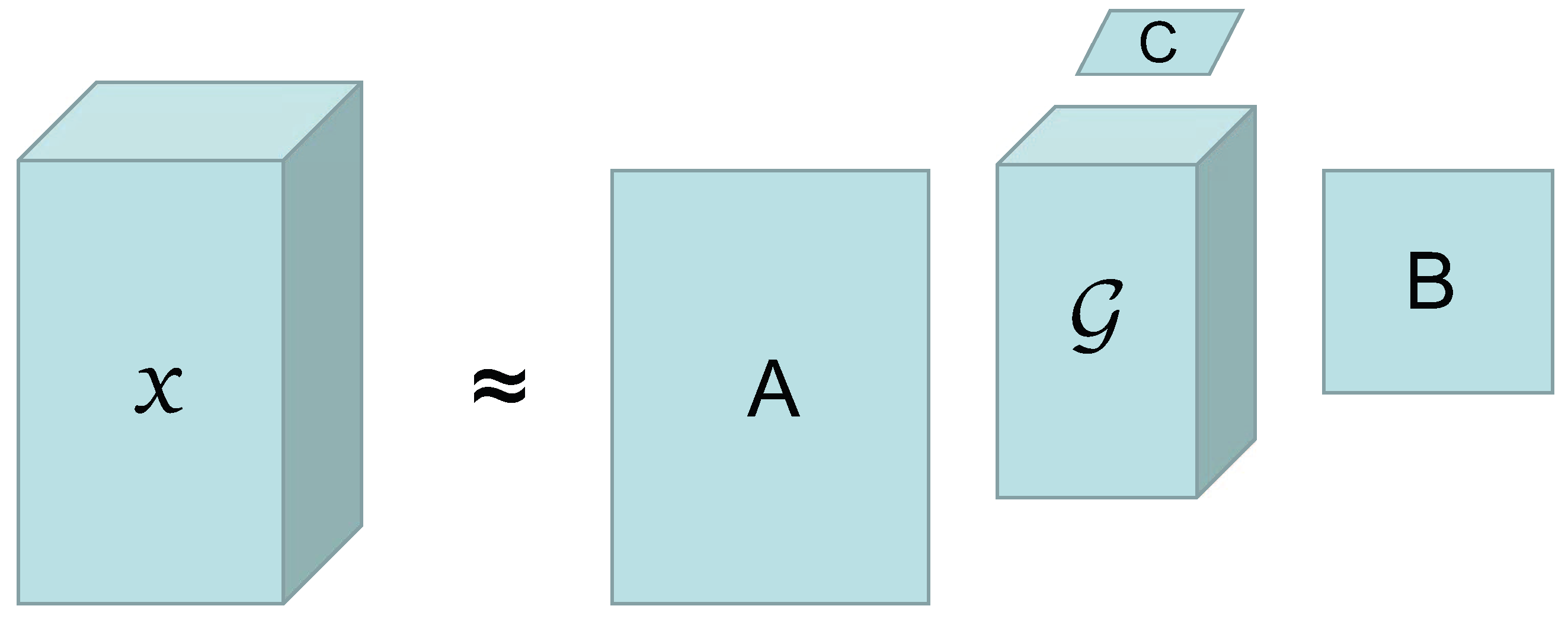
Therefore, in this paper, the Tucker decomposition method is used to illustrate the low-rank prior of HSIs in spectral and spatial dimensions. Taking a third-order tensor of rank as an example, a core tensor and factor matrices , , and in three directions can be obtained by Tucker decomposition, as shown in Figure 1. The mathematical form of its decomposition can be written as:
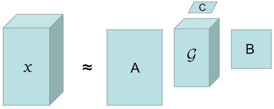
Figure 1.
Diagrammatic presentation of a third-order tensor’s Tucker decomposition.
2.3. HSSTV
HSSTV [41], as a higher-order TV, provides a deeper excavation of spectral and spatial higher-order sparsity. Compared with ASSTV, HSSTV is able to simultaneously handle both spatial difference information and spatial-spectral difference information within the HSI. Besides, it can also eliminate similar noises between adjacent bands that cannot be eliminated by ASSTV. Meanwhile, HSSTV has a strong ability to eliminate noise and artifacts while avoiding over-smoothing issues. It can achieve a good denoising effect without combining with other regularization methods. And HSSTV is defined as
where , is the spatial gradient operator with and being the vertical and horizontal gradient operators, is the spectral gradient operator; is the mixed norm, when calculating, which translates the gradient tensors into a four-row matrix, and then the matrix norm algorithm is used. When , the mixed norm is norm, and when , the mixed norm is norm.
In order to better understand the sparsity of the HSSTV, we do gradient processing on HSI data along with vertical, horizontal, vertical spectral, and horizontal spectral directions, and unfold along the spectral direction, finally the four plots shown in Figure 2 are obtained. From the figure, we can see that the color of most areas is blue, which indicates that most of the values are close to zero or zero. Moreover, the color of each row is almost the same, indicating that the row is either all zero or all non-zero, which proves that the gradient domain of HSI has group sparsity. Also, counting the data after the four directional gradients yields the four histograms in the second row of Figure 3, which shows that most of the data are zero. Compared to the ASSTV, the difference values of HSSTV are closer to zero, and the sparsity is more obvious. At the same time, HSSTV adds a portrayal of spatial sparsity to SSTV. Therefore, HSSTV can provide a more approximate sparse prior representation in both spatial and spectral domains.
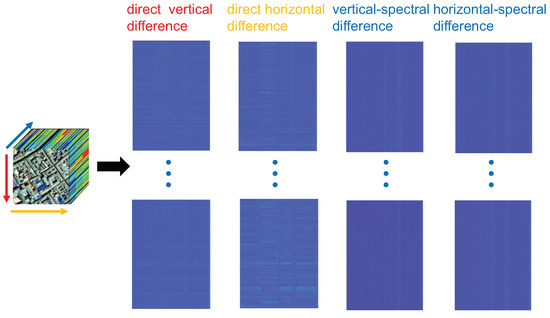
Figure 2.
The group sparsity of HSSTV.
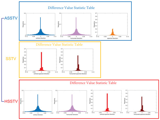
Figure 3.
The sparsity comparison of ASSTV, SSTV and HSSTV.
3. Proposed Method
3.1. GHSSTV Regularization
The gradient domain of HSI is sparse. TV regularization can effectively explore smoothing information of HSIs and describe their sparse prior. For example, ASSTV and SSTV regularization terms use the norm to describe the sparsity of the gradient domain. And HSSTV uses the norm to explore the sparsity of the gradient domain. However, HSI data has its characteristics in the gradient domain. In other words, at each band of HSIs, the gradient values in boundary areas are significantly big, while the ones in smooth areas are small. This characteristic can be referred to as group sparsity in the gradient domain of HSIs, as shown in Figure 2. The norm or norm does not reflect this characteristic of HSIs. Without further sparsity requirements on the features of the internal structure, the norm simply requires the sum of the absolute values of all elements to be minimal. Compared with the norm, although the norm can prevent overfitting and is more sensitive to particular points, the norm still does not require sparsity at a deeper level of structure. The norm combines the advantages of the norm and norm, and can well describe the characteristics of HSI in the gradient domain. On the one hand, the norm can ensure that each tube of the spectral dimension of the gradient tensor is sparse. On the other hand, sparsity in the spatial dimension can also be guaranteed. The norm of the gradient domain can be written as:
where D is the gradient operator. In order to describe the group sparsity with the norm, we propose the GHSSTV regularization term to ensure that it is sparse in the spectral dimension and spatial dimension, i.e.,
where , ; ; and represent local spatio-spectral differences operators; and represent direct local spatial differences operators. The specific form of GHSSTV regularization can be written as follows:
When and are 0, GHSSTV degenerates into the TV term in the [40]. Compared with the TV term in the [40], we add a second-order TV, as can be seen in Figure 2, the sparse characteristics of the HSI data after the second-order gradient are more obvious. So the newly proposed TV regularization term can more comprehensively describe the sparse characteristics of HSI data.
Figure 3 shows the sparsity structure of HSI data obtained after three classical difference operators. The mathematical forms of the three TV regularizations are as follows:
where represents the weights of the three differences , and ; w represents the weight of equilibrium first-order D and second-order differences . As can be seen from the three equations, ASSTV only deals with first-order gradient, which can only represent the correlation between adjacent bands in the same dimension. There is no way to tap into the high-order gradient information of the HSI. Although ASSTV can describe the piecewise smoothness of HSI in both spatial and spectral dimensions, it is obviously insufficient compared with the other two TVs. As shown in Figure 3, SSTV and HSSTV represent more sparsity in histograms of high-order gradients. SSTV only deals with second-order TV, which is able to obtain more correlations between bands near different dimensions compared to first-order TV. However, SSTV does not explore first-order gradient information in the spectral and spatial dimensions. This makes SSTV lack much of the information that can be obtained directly and lead to spatial over-smoothing. Although HSSTV not only retains the exploration of spatial and spectral correlation by first-order TV of ASSTV but also has the mining of high-order gradient structures by second-order TV. The norm cannot describe the structural sparsity of HSI. The proposed GHSSTV not only explores the information of first-order gradient and high-order gradient but also reasonably describes the group sparsity of HSI.
3.2. New GHSSTV-Based Denoising Model
Here, we use the GHSSTV regularization to fully explore the local smoothing structure in the spatial and spectral domains. At the same time, combining the low-rank characteristics of a clean HSI can effectively remove the mixing noise. Based on the above discussion, in this section, we propose a new HSI denoising model by combining GHSSTV with Tucker decomposition, that is,
where is the Tucker decomposition, is referred to as the core tensor after decomposition and is referred to as the factor matrices; is the sum of the absolute values of all elements; is the inner product of the tensor. When the values of , , and are 0, the model can degenerate into LRTDGS model.
As reviewed in Equation (10), the sparse constraints on the HSI gradient domain can effectively eliminate mixed noises. In addition, the use of the Frobenius norm to model Gaussian noise enables denoising for real situations with severe Gaussian noise. It is easy to see that the new model must be very good at denoising. Besides, the above problem (10) is a non-convex optimization problem, so it is possible to find a good local solution through the ADMM algorithm.
3.3. Optimization
It is difficult to solve the problem directly because of its non-convex property. Here, we resort to the algorithmic framework of ADMM for the solution. To facilitate the solution, we first introduce two variables and . The model (10) is rewritten as
Collating the constraints of the above problem and transforming the constrained optimization problem (11) into an unconstrained optimization problem (12),
In Equation (12) we use to denote the penalty parameter and to represent the Lagrange multiplier in the ADMM algorithm. The main idea of the ADMM algorithm is to decompose a large global problem into several smaller, more easily solvable local subproblems, and to obtain the solution to the large global problem by coordinating the solutions of the subproblems. Thus, the next step is to work on the sub-problems first.
(1) .
And by calculating this, we can get:
Combined with the HOOI algorithm, and can be computed, and thus can be calculated to obtain.
(2) .
After calculation, the solution can be obtained as Formula (17):
where represents the adjoint operator of A. In order to solve Formula (17), we need to use the FFT matrix [45]. Then, we obtain
where ; is the fast Fourier transform, is its inverse transform; And means that the square of each element needs to be calculated.
(3) .
After calculation, we can obtain:
Assuming , in order to solve for , based on [46], we can use the following formula.
Among them, the expression method of is as follows:
(4) .
Similarly, we can get:
We use the soft-thresholding operator to update :
(5) .
Through the calculation of Equation (26), we can get the ultimately needed .
(6) . The iterative formula for the multiplier is as follows:
where is set to 0.01, . Through continuous iteration of solving the above sub-problems, we can obtain the final required HSI . The specific calculation process is shown in Algorithm 1.
| Algorithm 1 The solution of GHSSTV |
| Input: The noisy HSI , desired rank for Tucker decomposition, the stopping criteria , the parameter , and the regularization parameters , and , |
| Initialize: Initial . |
| Output: The restored HSI . |
| while not converge do |
| 1. Update , by Equation (15) and Equation (18), respectively. |
| 2. Update , by Equation (21) and Equation (25), respectively. |
| 3. Update , Multipliers by Equation (27) and Equation (28), respectively. |
| 4. Check the the convergence condition |
| end while |
3.4. Computational Complexity Analysis
In this section, we analyze the computational complexity of the proposed method. Assume that the size of the input HSI data is , first, the HOOI algorithm is used to update and subproblems. This mainly includes the implementation of SVDs algorithm and tensor matrix product operation. To simplify analysis, we set the Tucker rank r to the same value. Then the total computational complexity of HOOI is [47]. In addition, the subproblem is optimized using FFT, and the computational complexity is . Finally, for the calculation of the , , and subproblems, since we have carried out gradients in four directions of the spatial and spectral dimensions, the computational complexity is . Considering all subproblems, the overall computational complexity of Algorithm per iteration is .
4. Experiments and Discussion
To verify the performance of the GHSSTV method in the field of noise removal, the GHSSTV model is applied to simulated data experiments and real data experiments, respectively. Furthermore, to demonstrate the superiority of the GHSSTV method, it is compared with seven highly effective denoising methods under the same conditions, including the WNNM model [14], the LRMR model [16], the WSNM model [15], the LRTV model [34], the LRTDTV model [39], the LRTDGS model [40], and the FGSLR model [26]. Before conducting the experiment, the grey values of each band of the HSI used need to be normalized to [0, 1]. After the experiment is completed, the grey values of each band are restored to their original values. The parameters used in each method are fine-tuned from the original optimal parameters to ensure the best results. And the selection of parameters for the GHSSTV method is described in detail in IV-C. In order to demonstrate more convincingly the superiority of the GHSSTV method, visual quality and evaluation indexes are used for comparative illustration.
4.1. Simulated Data Experiments
In this section, two hyperspectral datasets are selected for simulation experiments. The first dataset is the Indian pine dataset [48], which has a spatial size of 145 × 145 and a total of 224 bands. The second dataset is the Pavia Centre dataset [49]. In this part, data sets with a space size of 200 × 200 and a total of 80 bands are selected for the experiment. To verify the effectiveness of the GHSSTV model in removing different types of noise, six different types of noise are added to the two datasets. The details are shown in Table 2.
Table 2.
Different noise scenarios for synthetic HSI data.
(1) Visual quality comparison:
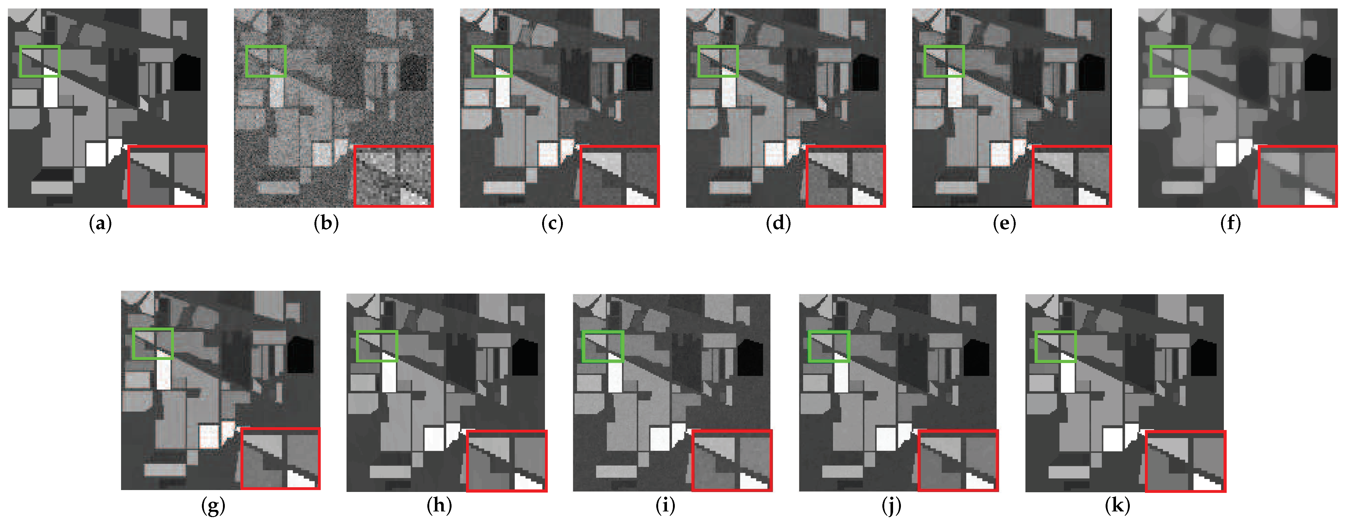
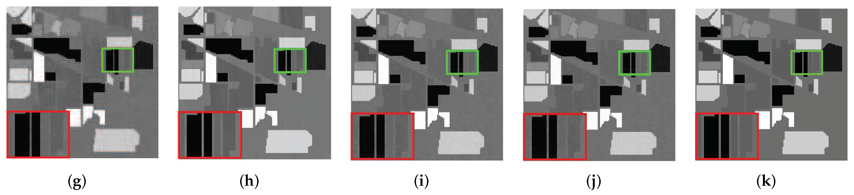
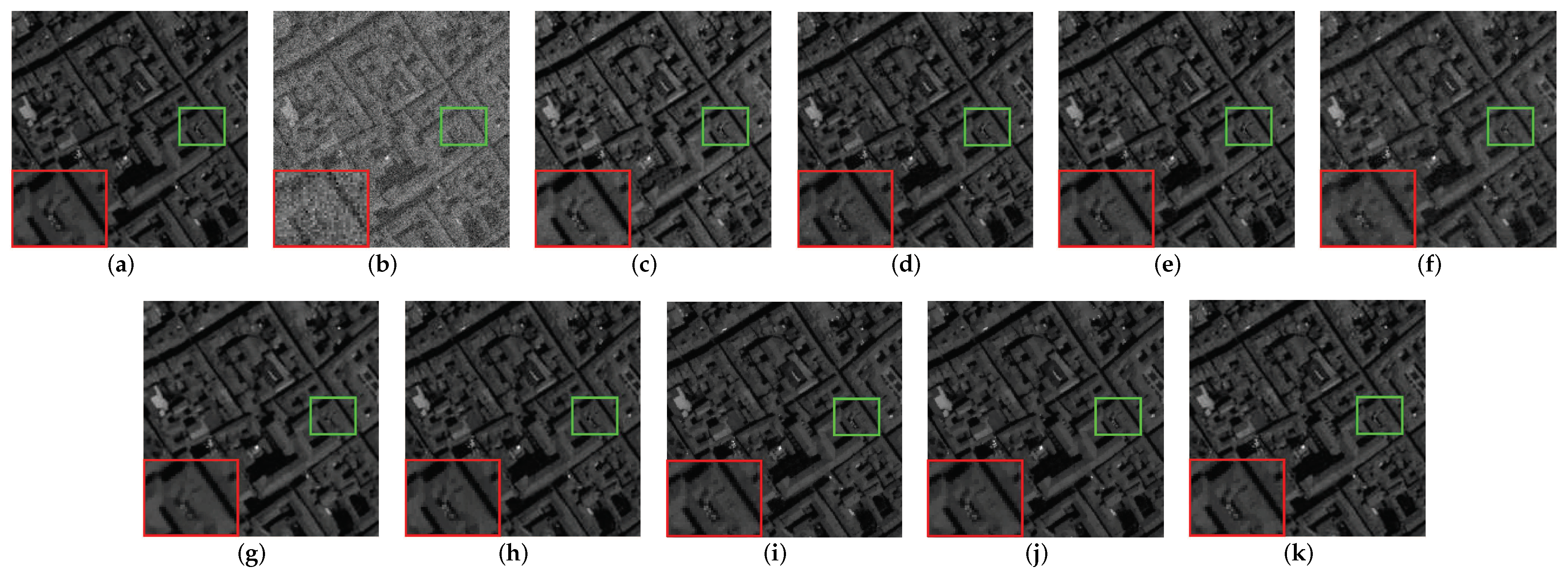
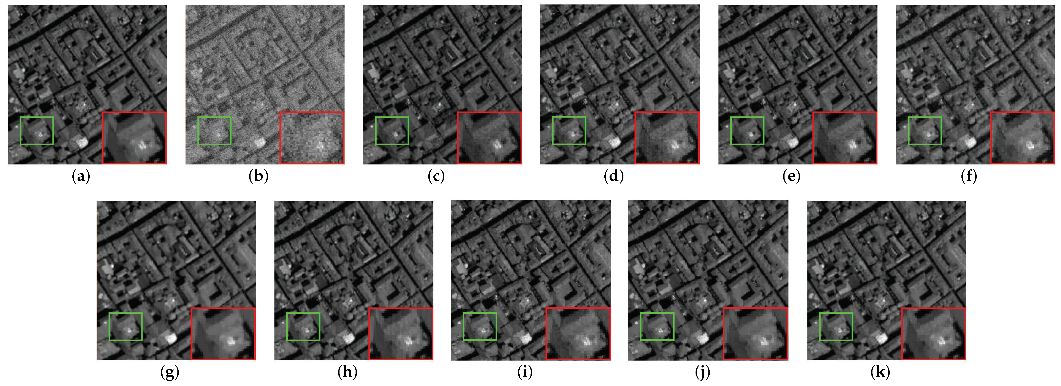
In this subsection, two representative HSI recovery bands are selected for each of the two simulation data in detail. The image comparison results are shown in Figure 4, Figure 5, Figure 6 and Figure 7. Regarding the simulated data based on the Indian pine dataset, Figure 4 illustrates the recovery effect of band 200 in the recovery results of HSI images that are mainly corrupted by noise case 1. In this case, the original HSI is mainly corrupted by strong Gaussian noise, as shown in Figure 4b. Figure 5 shows the results of the recovery effect of the HSI image in band 129, which is mainly corrupted by noise case 5. Here the original HSI is corrupted by Gaussian noise, impulse noise, and deadlines. Compared to noise case 1, the noise situation is much messier, which can be seen in Figure 5b. For Pavia Centre-based simulation data, Figure 6 shows the recovery effect of band 30 disrupted by noise case 3. Figure 7 shows the recovery effect of band 73 disrupted by noise case 6. The main noises removed in Figure 6 are Gaussian noise and impulse noise. On this basis, Figure 7 also needs to remove deadlines and strips. The situation after adding noise are shown in Figure 6b and Figure 7b. To display the denoising situation of each method more clearly, we zoom in at the specific area in the image and highlight the marked original area with a green box and the marked enlarged area with a red box.

Figure 4.
The comparison of the effect of band 200 before and after denoising in the simulated data experiment: (a) original image, (b) noisy image, (c) WNNM, (d) LRMR, (e) WSNM, (f) LRTV, (g) LRTDTV, (h) LRTDGS, (i) , (j) , (k) Novel GHSSTV method.
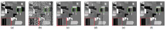
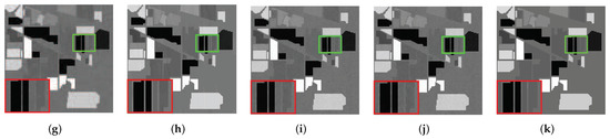
Figure 5.
The comparison of the effect of band 129 before and after denoising in the simulated data experiment: (a) original image, (b) noisy image, (c) WNNM, (d) LRMR, (e) WSNM, (f) LRTV, (g) LRTDTV, (h) LRTDGS, (i) , (j) , (k) Novel GHSSTV method.
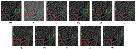
Figure 6.
The comparison of the effect of band 30 before and after denoising in the simulated data experiment: (a) original image, (b) noisy image, (c) WNNM, (d) LRMR, (e) WSNM, (f) LRTV, (g) LRTDTV, (h) LRTDGS, (i) , (j) , (k) Novel GHSSTV method.
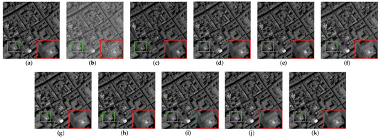
Figure 7.
The comparison of the effect of band 73 before and after denoising in the simulated data experiment: (a) original image, (b) noisy image, (c) WNNM, (d) LRMR, (e) WSNM, (f) LRTV, (g) LRTDTV, (h) LRTDGS, (i) , (j) , (k) Novel GHSSTV method.
In general, it can be easily seen from the results of the nine denoising methods in Figure 4 that GHSSTV has the best denoising effect, which achieves almost the same effect as the original image and removes the Gaussian noise very cleanly. At the same time, important information and edge details are perfectly preserved. Although the LRTDTV, LRTDGS, and perform better for removing most of the Gaussian noise, the recovered images are not particularly clear and the edge of them are blurred. In addition, LRTV can remove Gaussian noise, but the image is still too smooth, and the texture information loss is obvious. The remaining methods did not effectively remove the Gaussian noise, and the noise in the image can be clearly seen. As the image shown in Figure 5 is subjected to more complex noise, most of the methods do not recover very well. However, the GHSSTV method continues to perform very consistently and effectively in removing the mixed noise. All areas of the image are recovered very cleanly, with sharp edges between them. Compared with GHSSTV, LRTDGS has artifacts and blurred edges in a small area. In addition, it can be seen from the graph that all methods except LRMR can effectively remove deadlines. In contrast, LRTV and LRTDTV are effective in removing Gaussian and impulse noise but do not retain edge information and detail. And the LRTDTV outperforms the LRTV, image smoothing phenomenon still exists in some regions of LRTV. WSNM, , and effectively remove impulse noise but have residual Gaussian noise. WNNM and LRMR do not effectively remove mixed noise and important information such as edges are not preserved. In Figure 6, GHSSTV, , , LRTDFGS and LRTDTV can effectively remove noise, but LRTDTV and LRTDGS lose more details. Other methods do not remove noise, especially LRTV has a large amount of residual Gaussian noise and impulsive noise. Among all the denoising methods shown in Figure 7, LRMR and LRTDGS still have the influence of deadlines. The WNNM, LRMR, WSNM and LRTV methods do not remove noise cleanly, and there are still obvious Gaussian noise and impulse noise. still has a small amount of Gaussian noise remaining. The image recovered by GHSSTV and are not much from the original image. In summary, GHSSTV outperforms the other methods in the simulated data experiments. It is able to perform very well in terms of noise removal and retention of edge information.
(2) Quantitative comparison:
To quantitatively evaluate restoration performance, we introduce three evaluation indexes, the mean peak signal to-noise ratio (MPSNR), which calculates the mean square error between the clean image and the denoised image, with larger values indicating better image recovery. The mean structural similarity index (MSSIM), which is able to illustrate the similarity between a clean image and a denoised image in terms of luminance, contrast, and structure respectively. Compared to MPSNR, the focus is more on comparison in terms of visual characteristics. Similarly, the higher the value, the better the image is restored. As well as the erreur relative globale adimensionnelle de synthèse (ERGAS), which calculates the relative error between the clean image and the denoised image, the smaller the value the better the image is recovered. they are defifined as follows:
where is the PSNR value of band i, is the SSIM value of band i; denotes the clean image of band i and denotes the recovered image of band i.
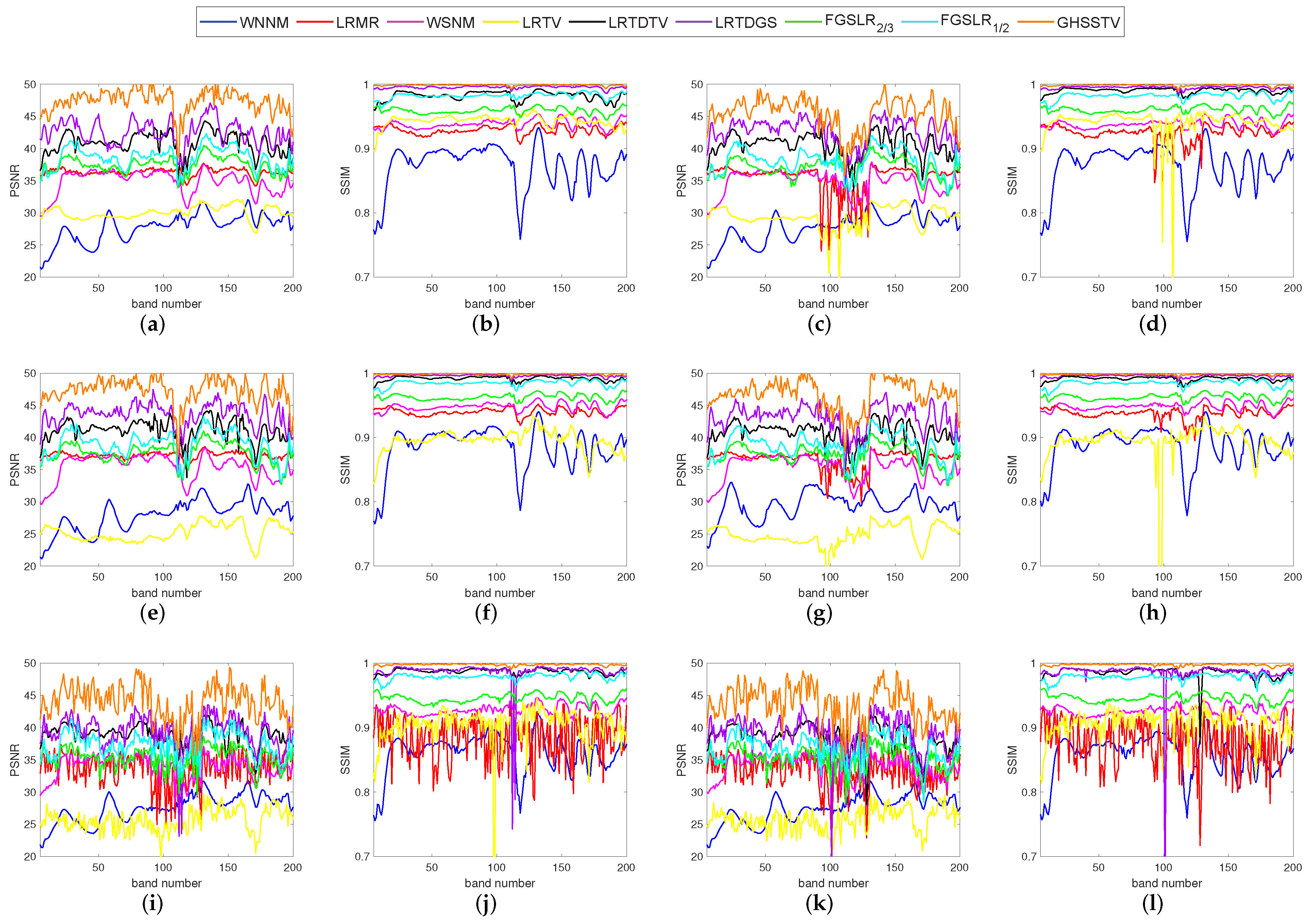
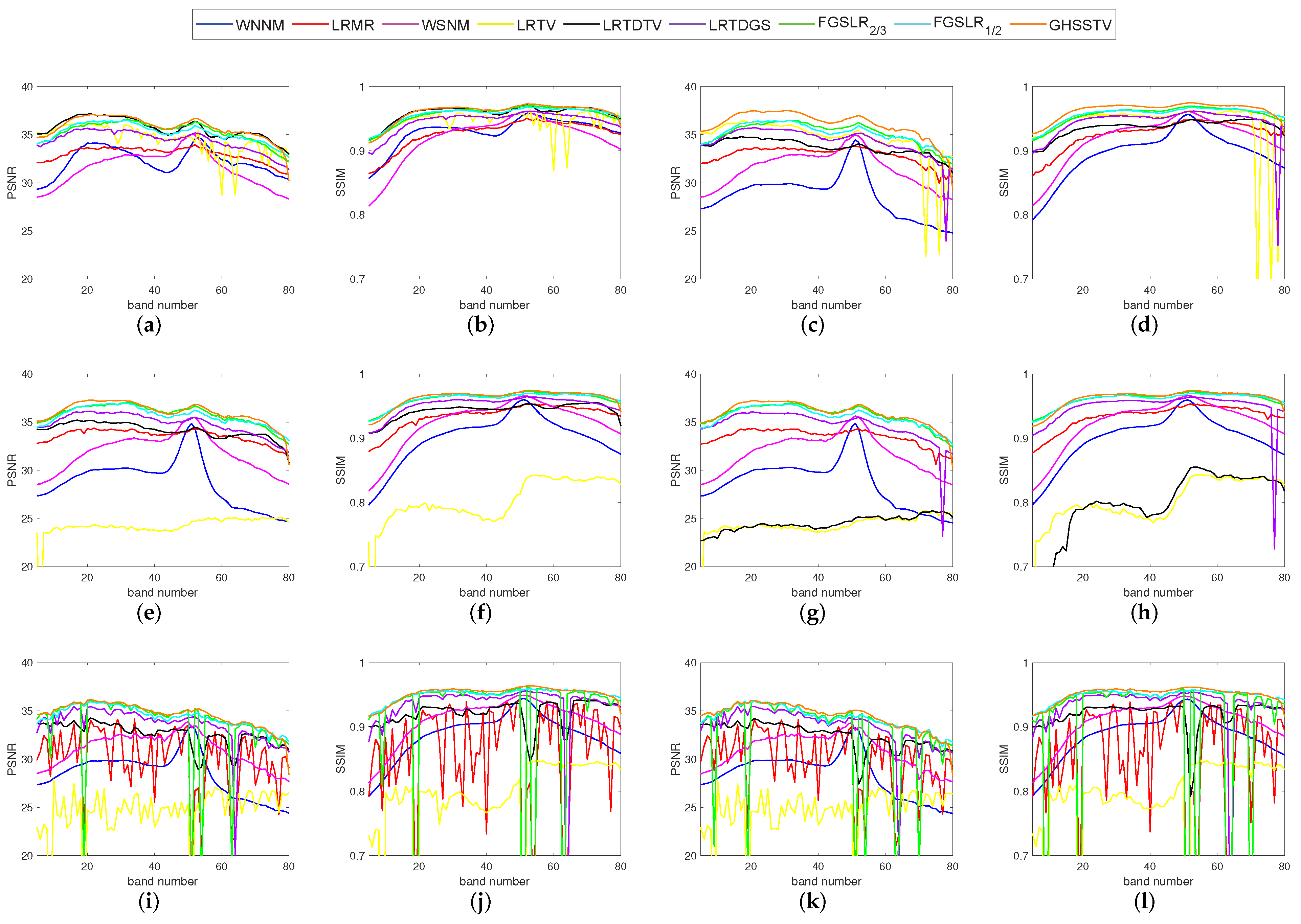
For the purpose of quantitative comparison, Table 3 records the recovery results of all comparison methods under the above three Picture Quality Indices (PQIs). For each type of noise, the index values with the best denoising effect are highlighted in bold. As can be seen from Table 3 and Table 4, GHSSTV has the best results, performing very well on all three PQIs mentioned. In order to get a detailed view of the comparison of PSNR and SSIM values for each band, Figure 8 and Figure 9 gives a comparison of the index values for each band when the nine methods are denoised for six different noise scenarios. It is easy to see that the GHSSTV method outperforms the other methods in all bands. The next best performer is the LRTDGS method. The other methods perform better and worse in each band for each of the six noise scenarios.
Table 3.
Comparison of three quantitative metrics for different HSI denoising methods in simulated dataset.
Table 4.
Comparison of three quantitative metrics for different HSI denoising methods in simulated dataset.
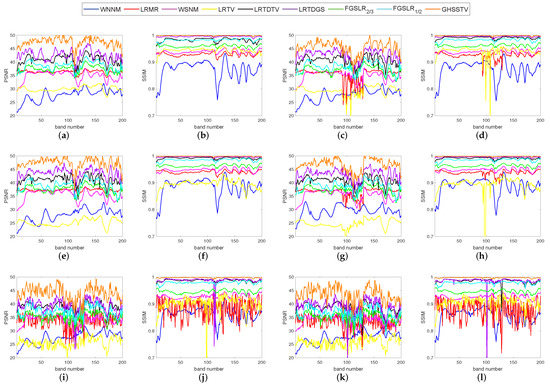
Figure 8.
Comparison of PSNR and SSIM values in each band in various denoising methods: (a,b) noise case 1, (c,d) noise case 2, (e,f) noise case 3, (g,h) noise case 4, (i,j) noise case 5, (k,l) noise case 6.
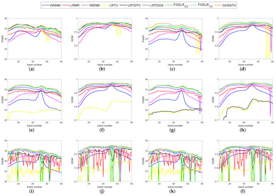
Figure 9.
Comparison of PSNR and SSIM values in each band in various denoising methods: (a,b) noise case 1, (c,d) noise case 2, (e,f) noise case 3, (g,h) noise case 4, (i,j) noise case 5, (k,l) noise case 6.
4.2. Real Data Experiments
In this section, two real HSI data sets, including the HYDICE urban data set [50] and the AVIRIS Indian Pines data set [48] are used to demonstrate the utility and superiority of the GHSSTV method. They are severely damaged by mixed noise. Therefore, restoring clean HSIs from them is a huge challenge.
(1) HYDICE Urban Data Set: It is a data set about the planning for different areas of the city, which size is . And it is a very classical data set for demonstrating denoising effects.
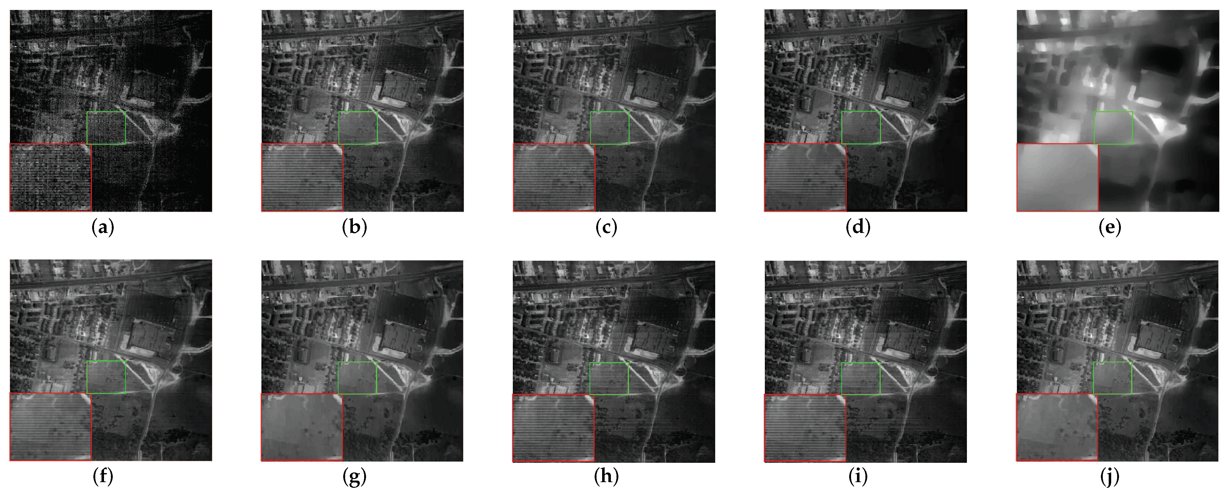
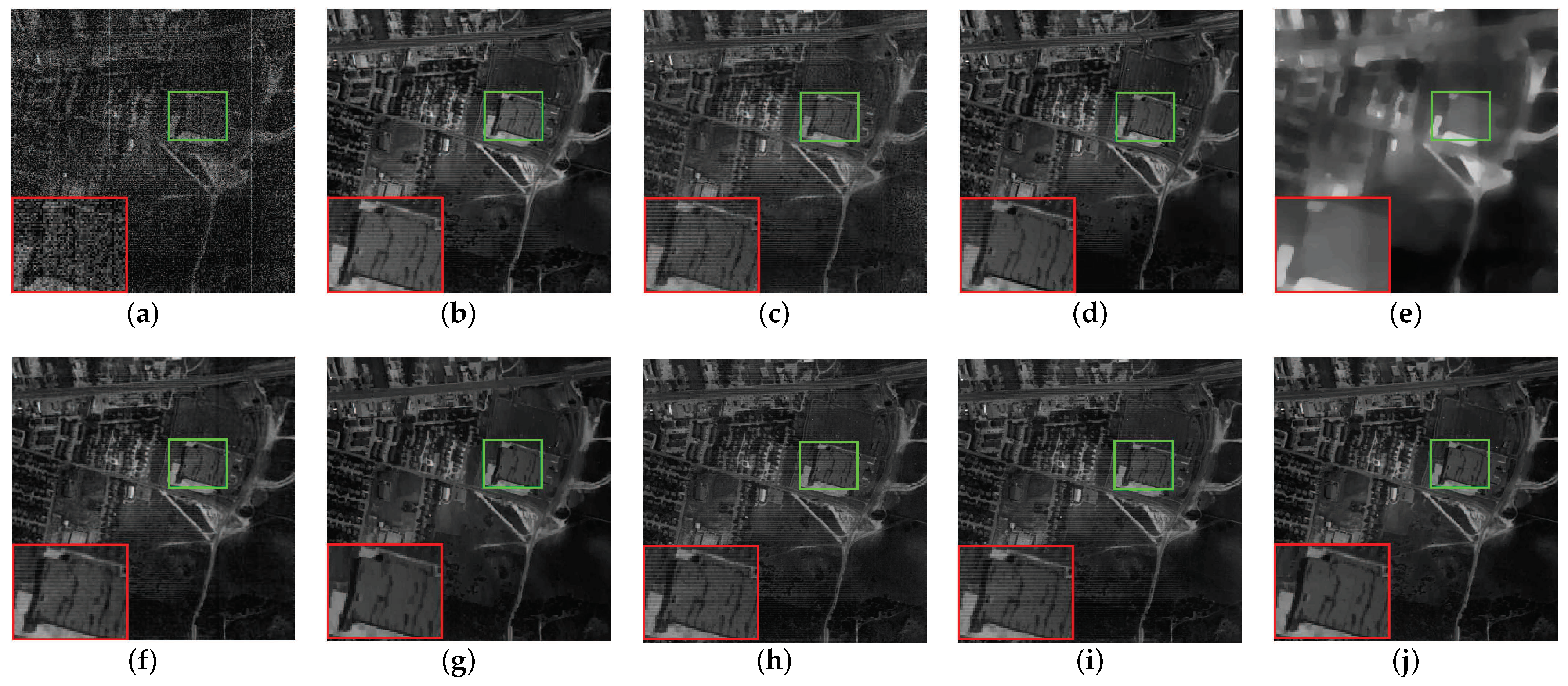
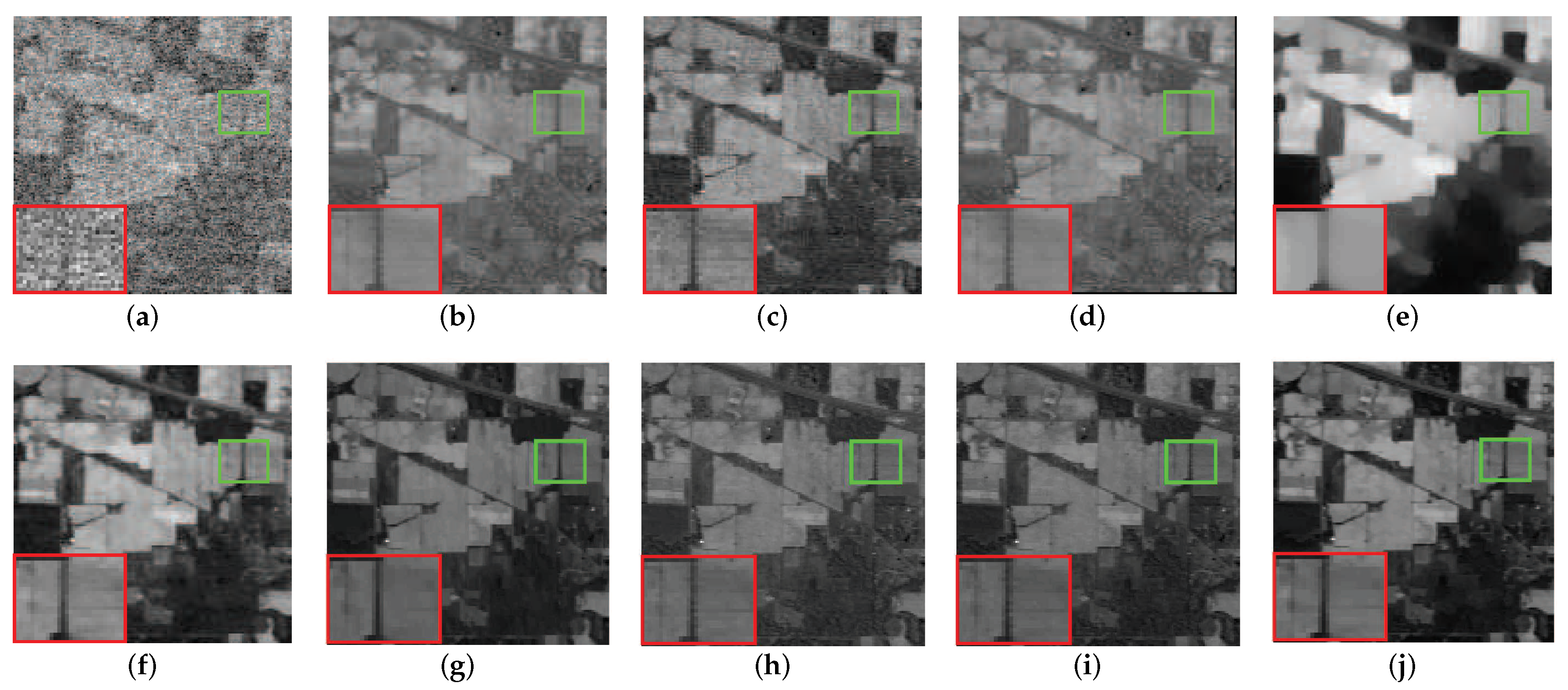
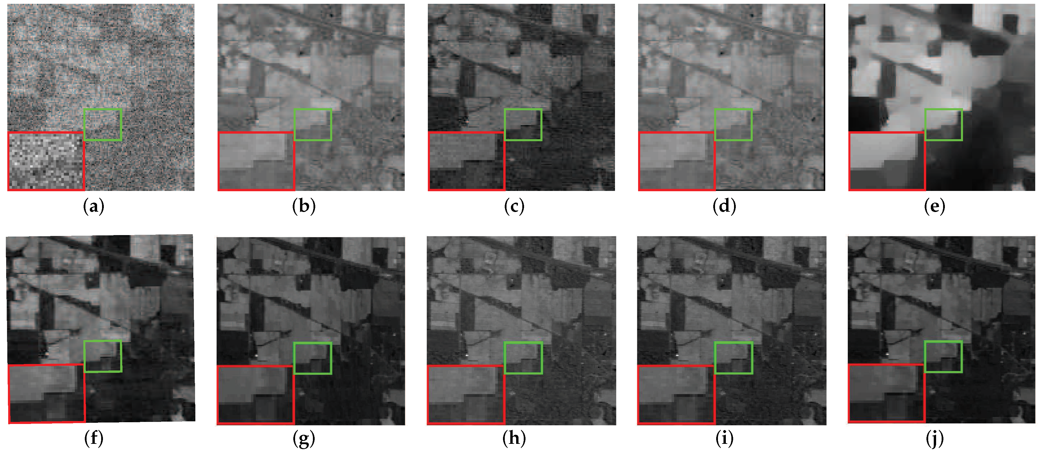
We selected two bands with obvious changes before and after denoising of HYDICE urban data set for demonstration and detailed analysis. As shown in Figure 10 and Figure 11, Figure 10 shows the comparison among the image of band 109 in the original data and the images of this band after denoising by nine methods. Figure 11 shows 10 images of band 207 before and after denoising. It can be easily seen from Figure 10 and Figure 11 that WNNM and LRMR are very good at removing Gaussian noise and dead lines, but they appear to be helpless for stripes. It is possible that strips typically only appear in specific locations within the specific frequency bands, which may be mistaken for clean low-rank content and not eliminated during model operation. Moreover, compared with the other method, LRMR has an over-smoothing phenomenon, and the boundary is ambiguous. LRTV can remove stripes, but there may be an over-smoothing phenomenon. The LRTDTV method is able to remove some of the strips compared to the above mentioned methods, but not all of them. In addition, it performs very well in the removal of other noise. and remove noises other than strips, but the remaining strips are clearly visible. The GHSSTV method is very effective at removing strips and is also very good at removing Gaussian noise and dead lines. Compared to the other methods, GHSSTV performs very well in terms of mixed noise removal.
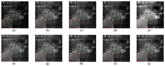
Figure 10.
The comparison of the effect of band 109 denoising before and after in the HYDICE Urban dataset experiment: (a) original image, (b) WNNM, (c) LRMR, (d) WSNM, (e) LRTV, (f) LRTDTV, (g) LRTDGS, (h) , (i) , (j) novel GHSSTV method.
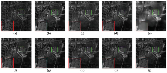
Figure 11.
The comparison of the effect of band 207 denoising before and after in the HYDICE Urban dataset experiment: (a) original image, (b) WNNM, (c) LRMR, (d) WSNM, (e) LRTV, (f) LRTDTV, (g) LRTDGS, (h) , (i) , (j) novel GHSSTV. method.
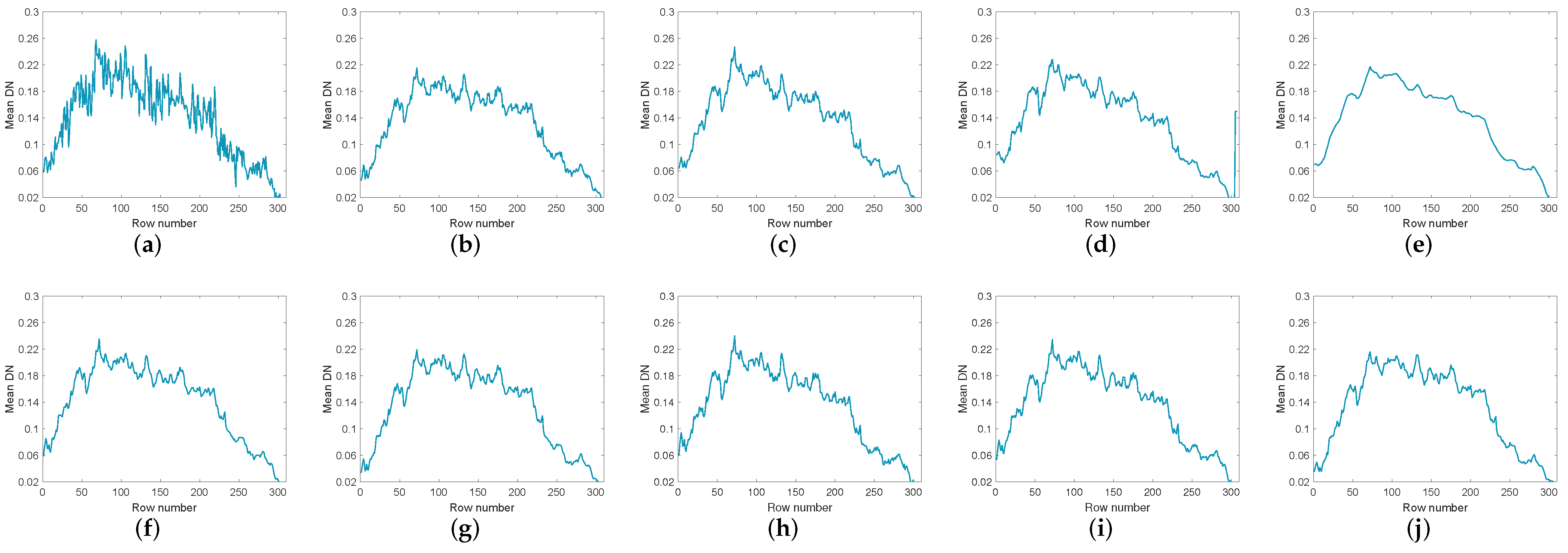
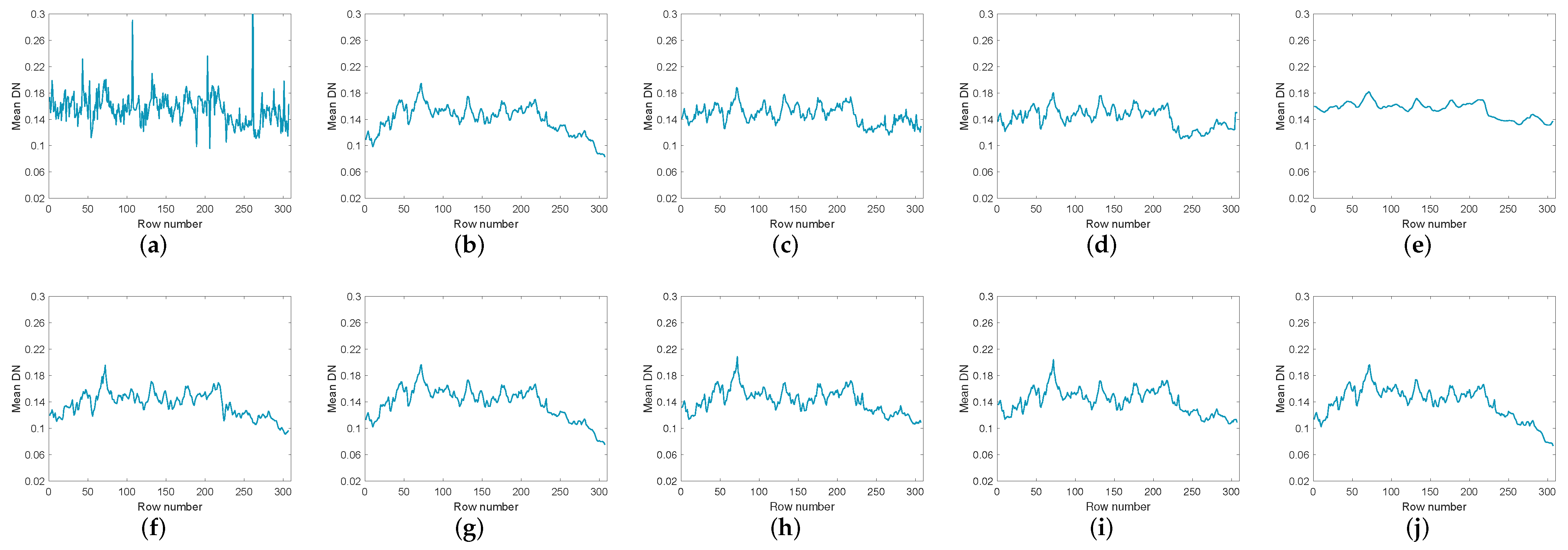
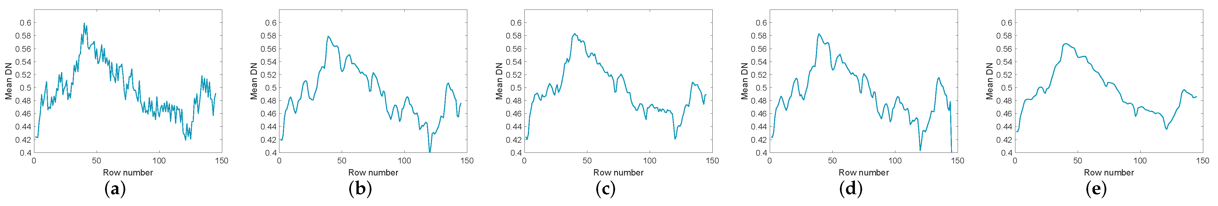
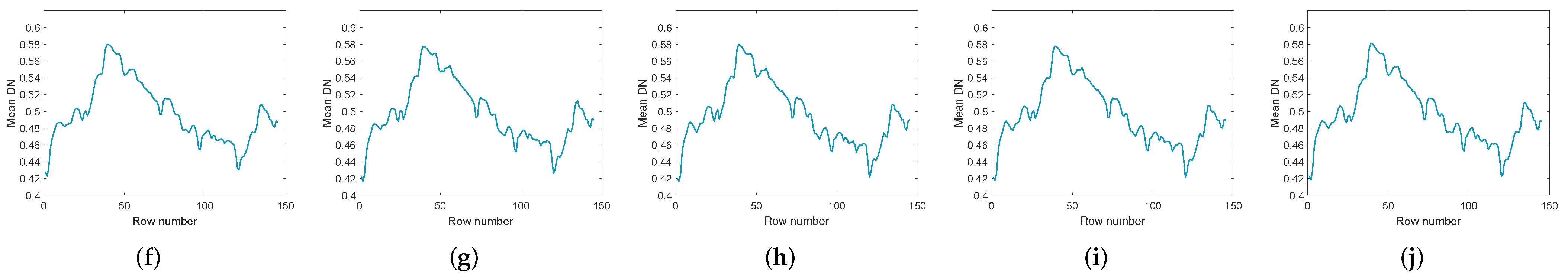
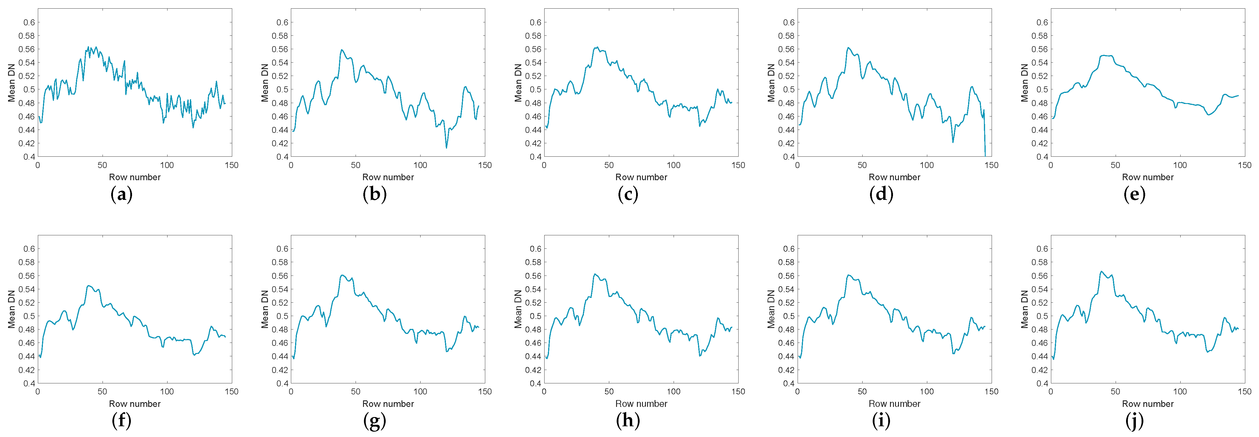
To compare the denoising effects of various methods more comprehensively, Figure 12 and Figure 13 list the vertical average cross-sectional views of the corresponding bands in Figure 10 and Figure 11 respectively. In Figure 12a and Figure 13a, the mean profiles fluctuate violently, indicating that there are serious noise in the images. Among the restored images of various methods, LRTV has the smoothest contour. However, LRTV obviously has excessive smoothing and loses a lot of useful information. The rest of the methods can effectively remove the noise, but there are still some local noises in the profiles. Relatively speaking, the contours in GHSSTV are the smoothest.
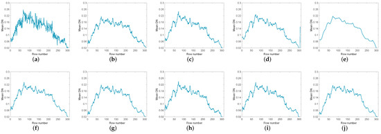
Figure 12.
The vertical mean profiles of band 109 by all the compared methods for the Urban dataset: (a) original image, (b) WNNM, (c) LRMR, (d) WSNM, (e) LRTV, (f) LRTDTV, (g) LRTDGS, (h) , (i) , (j) novel GHSSTV method.
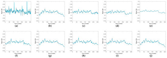
Figure 13.
The vertical mean profiles of band 207 by all the compared methods for the Urban dataset: (a) original image, (b) WNNM, (c) LRMR, (d) WSNM, (e) LRTV, (f) LRTDTV, (g) LRTDGS, (h) , (i) , (j) novel GHSSTV method.
(2) AVIRIS Indian Pines Data Set: Its original size is . The data set presents realistic scenarios of the situation in and around the pine forest.
Figure 14 and Figure 15 compare the images of the original data and the data after denoising by different methods in band 109 and band 219 respectively. After denoising, it is easy to observe that the denoising effect of low-rank matrix methods like WNNM, LRMR, and WSNM is not obvious. In contrast, the WNNM model and the WSNM model outperform the other method in terms of removing strong Gaussian noise, but they have the disadvantage that the boundary is blurred due to obvious overfitting. When the noise is heavy, these methods even appear the degradation of gray value. For LRTV, it would over-smooth the image, causing the structure to change. LRTDTV, , and can remove lots of noise, but there may be over smoothing phenomenon in local details. GHSSTV can still obtain the best noise reduction performance and effectively avoid over smoothing and spectral distortion. It can also be seen from Figure 16 and Figure 17, The line of LRTV is too smooth, and the local fluctuations of WNNM, LRMR, WSNM, LRTDTV, , and are obvious. LRTDGS works similarly to GHSSTV. However, GHSSTV performs better in detail, and GHSSTV has a smoother profile.
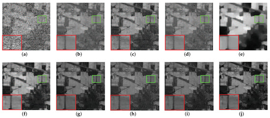
Figure 14.
The comparison of the effect of band 109 denoising before and after in the Indian pines dataset experiment: (a) original image, (b) WNNM, (c) LRMR, (d) WSNM, (e) LRTV, (f) LRTDTV, (g) LRTDGS, (h) , (i) , (j) novel GHSSTV method.
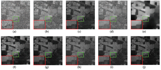
Figure 15.
The comparison of the effect of band 219 denoising before and after in the Indian pines dataset experiment: (a) original image, (b) WNNM, (c) LRMR, (d) WSNM, (e) LRTV, (f) LRTDTV, (g) LRTDGS, (h) , (i) , (j) novel GHSSTV method.
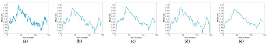
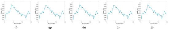
Figure 16.
The vertical mean profiles of band 109 by all the compared methods for the Indian pines dataset: (a) original image, (b) WNNM, (c) LRMR, (d) WSNM, (e) LRTV, (f) LRTDTV, (g) LRTDGS, (h) , (i) , (j) novel GHSSTV method.
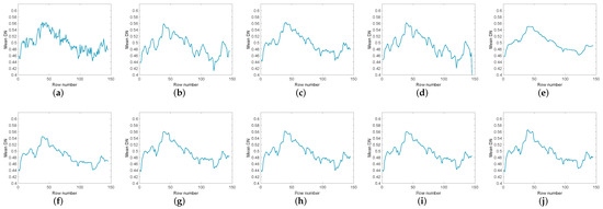
Figure 17.
The vertical mean profiles of band 219 by all the compared methods for the Indian pines dataset: (a) original image, (b) WNNM, (c) LRMR, (d) WSNM, (e) LRTV, (f) LRTDTV, (g) LRTDGS, (h) , (i) , (j) novel GHSSTV method.
4.3. Application for HSI Classification
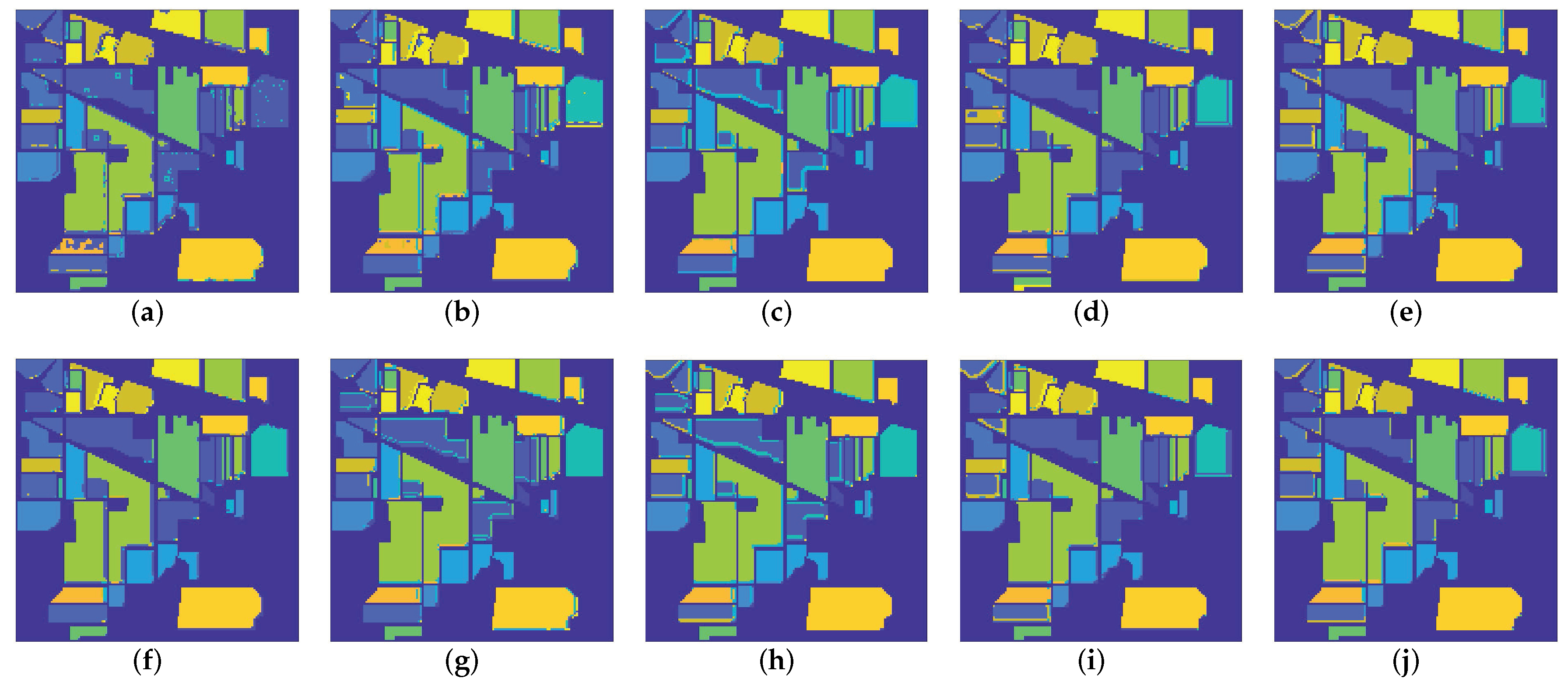
To illustrate the significant effect of denoising on subsequent applications such as classification, and to verify the characteristic reservation ability of the proposed method. In this section, we select the Indian pines dataset [48] with noise case 6 for classification experiments. The 3-dimensional discrete wavelet transform (3D-DWT) method [51] is adopted to classify the HSIs before and after denoising. To show the effectiveness of the GHSSTV method, we compare all the competing methods mentioned above. All of the above methods use overall accuracy (OA) and average accuracy (AA) [52] for numerical comparison, where OA represents the proportion of correctly classified samples to the total number of test samples, and AA represents the average of individual classification accuracy. Moreover, the classification maps for all the competing methods are shown in Figure 18, and the classification accuracy of various methods before and after denoising are reported and compared in Table 5. From Figure 18 and Table 5, it can be easily observed that the accuracy of the classification results after denoising has been significantly improved. In addition, the HSI classification results after denoising by the GHSSTV method are better than other methods.
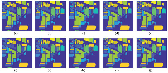
Figure 18.
Classification maps for all the competing methods on Indian pines dataset: (a) Noisy image, (b) WNNM, (c) LRMR, (d) WSNM, (e) LRTV, (f) LRTDTV, (g) LRTDGS, (h) , (i) , (j) novel GHSSTV method.
Table 5.
Classification accuracy (percentage) of all competing methods on the indian pines data set.
4.4. Discussion
Next, we will discuss model parameters and convergence.
(1) Sensitivity Analysis of Parameter : In the GHSSTV model, there are three important parameters to be determined. Considering the fact that , , and have certain proportional relationship. In general, we simply set the parameter as 1, which emphasizes the sparsity of the gradient domain. For the Frobenius term parameter that simulates Gaussian noise, unlike RPCA [13], the parameter is set to 10,000 or 20,000 based on previous experience and multiple trials. Through repeated experiments, 3 or 4 are selected as parameter to balance the effect of the sparse noise in the GHSSTV model. Under such parameter Settings, our model achieves the best results.
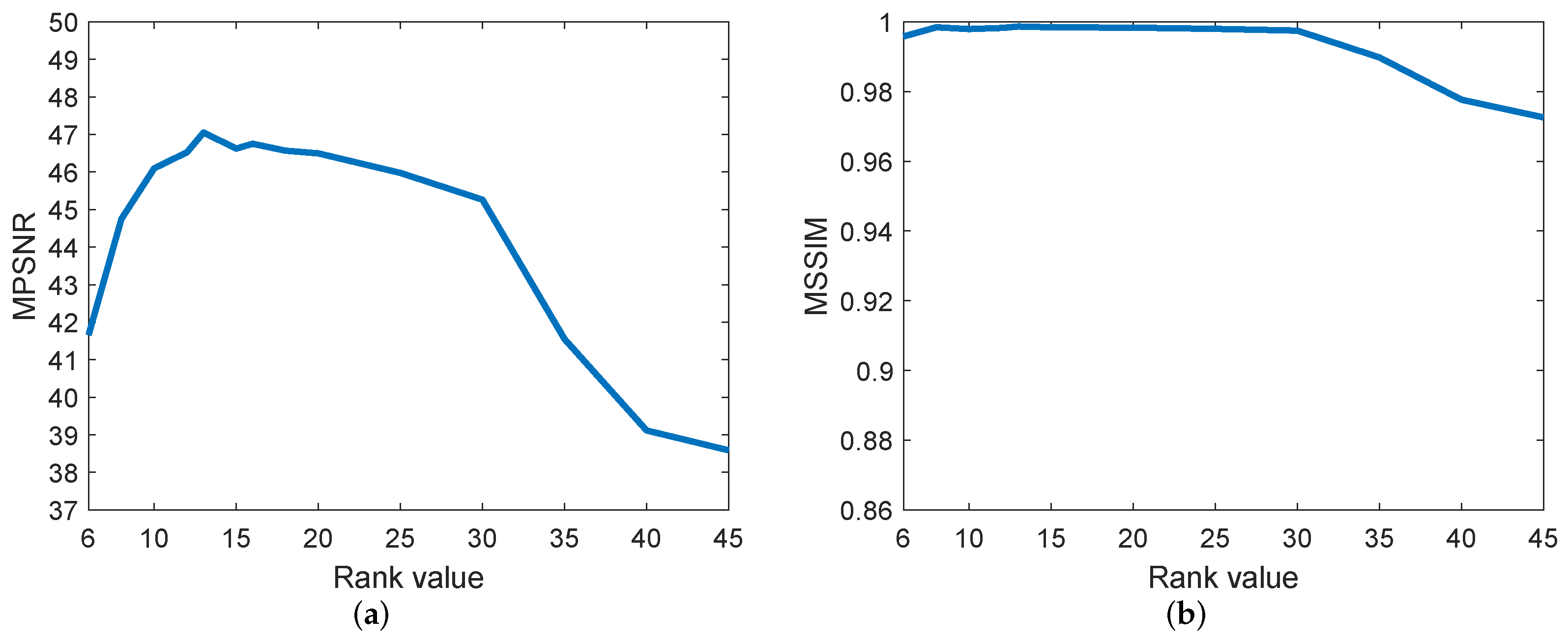
(2) Effectiveness of the Rank Constraint: For 3-D images, we need to give the estimated rank of three directions by using Tucker decomposition. The first two values correspond to two spatial modes, and typically the values are set to eighty percent of the length and width respectively. The third value is generally between 5 and 20. Figure 19 shows the curves for the variation of the evaluation index MPSNR and MSSIM values with the size of the rank. From Figure 19, we can find the most suitable value accurately.
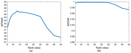
Figure 19.
MPSNR and MSSIM values change with spectral rank in the simulated Indian pines data experiment. (a) MPSNR value, (b) MSSIM value.
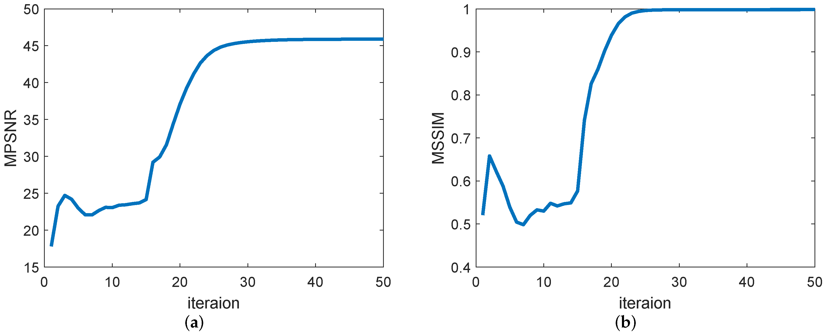
(3) Convergence analysis: Figure 20 shows the changes in the values of the evaluation indicators MPSNR and MSSIM as the number of iterations of the GHSSTV method. It is easy to see that when the number of iterations is around 30, the curve no longer rises but tends to be stable, which indicates that the algorithm is convergent.

Figure 20.
MPSNR and MSSIM values change with the number of iterations in the simulated Indian pines data experiment. (a) MPSNR value, (b) MSSIM value.
(4) computational time comparison: All the experiments are conducted in MATLAB 2019a with an Intel i5 CPU at 2.9GHz and 16 GB of memory. For the Indian Pine data set with size and Pavia data set with size , we average the time taken by the two groups of simulation experiments to achieve the best effect under the condition of noise case 1–6. The average running time of various methods is shown in Table 6. It should be noted here that the method proposed in this paper can achieve good results when it is iterated about 45 times. In order to get the best results this method can achieve, Table 6 shows the time taken for for 50 and 2500 iterations, respectively.
Table 6.
The average running time (in seconds) of different methods in the simulation experiment.
5. Conclusions
In this paper, we propose the GHSSTV model based on the group sparsity property of HSI in four directions of HSSTV. The new model performs very well in image denoising. It is worth mentioning that we use a norm for the tensor of the gradient domain, which guarantees the sparsity of clean images in both the spectral and spatial directions. This makes the GHSSTV method outstanding in removing sparse noise. In addition, we use the Frobenius norm term to simulate severe Gaussian noise. Finally, Through a series of experiments, it is proved that the GHSSTV method has obvious advantages over other classical denoising methods. In the future, we will further optimize the model and investigate the low-rank characteristics of the gradient-domain to enhance its ability to remove more complex noise in some real scenes.
Author Contributions
Conceptualization, P.Z.; methodology, P.Z.; writing—original draft preparation, P.Z.; writing—review and editing, P.Z. and J.N.; funding acquisition, J.N. All authors have read and agreed to the published version of the manuscript.
Funding
This research was funded by the National Key Research and Development Program of China under Grant 2017YFC0403302.
Institutional Review Board Statement
Not applicable.
Informed Consent Statement
Not applicable.
Data Availability Statement
Publicly available datasets were analyzed in this study. “AVIRIS Indian Pines data set” at https://engineering.purdue.edu/biehl/MultiSpec/hyperspectral.html, accessed on 8 March 2021; “HYDICE urban data set” at http://www.tec.army.mil/hypercube, accessed on 8 March 2021; “Pavia Centre dataset” at http://www.ehu.eus/ccwintco/index.php/, accessed on 8 March 2021.
Conflicts of Interest
The authors declare no conflict of interest.
References
- Bioucas-Dias, J.M.; Plaza, A.; Camps-Valls, G.; Scheunders, P.; Nasrabadi, N.; Chanussot, J. Hyperspectral remote sensing data analysis and future challenges. IEEE Trans. Geosci. Remote Sens. 2013, 1, 6–36. [Google Scholar] [CrossRef] [Green Version]
- Goetz, A.F. Three decades of hyperspectral remote sensing of the earth: A personal view. Remote Sens. Environ. 2009, 113, S5–S16. [Google Scholar] [CrossRef]
- Willett, R.M.; Duarte, M.F.; Davenport, M.A.; Baraniuk, R.G. Sparsity and structure in hyperspectral imaging: Sensing, reconstruction, and target detection. IEEE Signal Process. Mag. 2013, 31, 116–126. [Google Scholar] [CrossRef] [Green Version]
- Rudin, L.I.; Osher, S.; Fatemi, E. Nonlinear total variation based noise removal algorithms. Phys. D Nonlinear Phenom. 1992, 60, 259–268. [Google Scholar] [CrossRef]
- Dabov, K.; Foi, A.; Katkovnik, V.; Egiazarian, K. Image denoising by sparse 3-d transform-domain collaborative filtering. IEEE Trans. Image Process. 2001, 16, 2080–2095. [Google Scholar] [CrossRef] [PubMed]
- Maggioni, M.; Katkovnik, V.; Egiazarian, K.; Foi, A. Nonlocal transform-domain filter for volumetric data denoising and reconstruction. IEEE Trans. Image Process. 2012, 22, 119–133. [Google Scholar] [CrossRef] [PubMed]
- Manjón, J.V.; Coupé, P.; Martí-Bonmatí, L.; Collins, D.L.; Robles, M. Adaptive non-local means denoising of mr images with spatially varying noise levels. J. Magn. Reson. Imaging 2010, 31, 192–203. [Google Scholar] [CrossRef] [Green Version]
- Xue, J.; Zhao, Y. Rank-1 tensor decomposition for hyperspectral image denoising with nonlocal low-rank regularization. In Proceedings of the 2017 International Conference on Machine Vision and Information Technology (CMVIT), Singapore, 17–19 February 2017; pp. 40–45. [Google Scholar]
- Peng, Y.; Meng, D.; Xu, Z.; Gao, C.; Yang, Y.; Zhang, B. Decomposable nonlocal tensor dictionary learning for multispectral image denoising. In Proceedings of the IEEE Conference on Computer Vision and Pattern Recognition (CVPR), Columbus, OH, USA, 23–28 June 2014. [Google Scholar]
- Bai, X.; Xu, F.; Zhou, L.; Xing, Y.; Bai, L.; Zhou, J. Nonlocal similarity based nonnegative tucker decomposition for hyperspectral image denoising. IEEE J. Sel. Top. Appl. Earth Obs. Remote Sens. 2018, 11, 701–712. [Google Scholar] [CrossRef] [Green Version]
- Xue, J.; Zhao, Y.Q.; Bu, Y.; Liao, W.; Chan, J.C.W.; Philips, W. Spatial-spectral structured sparse low-rank representation for hyperspectral image super-resolution. IEEE Trans. Image Process. 2021, 30, 3084–3097. [Google Scholar] [CrossRef]
- Zhang, H.; Liu, L.; He, W.; Zhang, L. Hyperspectral image denoising with total variation regularization and nonlocal low-rank tensor decomposition. IEEE Trans. Geosci. Remote Sens. 2019, 58, 3071–3084. [Google Scholar] [CrossRef]
- Candès, E.J.; Li, X.; Ma, Y.; Wright, J. Robust principal component analysis? J. ACM 2011, 58, 1–37. [Google Scholar] [CrossRef]
- Gu, S.; Zhang, L.; Zuo, W.; Feng, X. Weighted nuclear norm minimization with application to image denoising. In Proceedings of the IEEE Conference on Computer Vision and Pattern Recognition (CVPR), Columbus, OH, USA, 23–28 June 2014; pp. 2862–2869. [Google Scholar]
- Xie, Y.; Qu, Y.; Tao, D.; Wu, W.; Yuan, Q.; Zhang, W. Hyperspectral image restoration via iteratively regularized weighted schatten p-norm minimization. IEEE Trans. Geosci. Remote Sens. 2016, 54, 4642–4659. [Google Scholar] [CrossRef]
- Zhang, H.; He, W.; Zhang, L.; Shen, H.; Yuan, Q. Hyperspectral image restoration using low-rank matrix recovery. IEEE Trans. Geosci. Remote Sens. 2013, 52, 4729–4743. [Google Scholar] [CrossRef]
- He, W.; Zhang, H.; Zhang, L.; Shen, H. Hyperspectral image denoising via noise-adjusted iterative low-rank matrix approximation. IEEE J. Sel. Top. Appl. Earth Observ. Remote Sens. 2015, 8, 3050–3061. [Google Scholar] [CrossRef]
- Cao, W.; Wang, Y.; Sun, J.; Meng, D.; Yang, C.; Cichocki, A.; Xu, Z. Total variation regularized tensor rpca for background subtraction from compressive measurements. IEEE Trans. Image Process. 2016, 25, 4075–4090. [Google Scholar] [CrossRef]
- Chang, Y.; Yan, L.; Chen, B.; Zhong, S.; Tian, Y. Hyperspectral image restoration: Where does the low-rank property exist. IEEE Trans. Geosci. Remote Sens. 2020, 59, 6869–6884. [Google Scholar] [CrossRef]
- Chang, Y.; Yan, L.; Zhao, X.-L.; Fang, H.; Zhang, Z.; Zhong, S. Weighted low-rank tensor recovery for hyperspectral image restoration. IEEE Trans. Cybern. 2020, 50, 4558–4572. [Google Scholar] [CrossRef] [Green Version]
- Chang, Y.; Yan, L.; Fang, H.; Zhong, S.; Liao, W. Hsi-denet: Hyperspectral image restoration via convolutional neural network. IEEE Trans. Geosci. Remote Sens. 2018, 57, 667–682. [Google Scholar] [CrossRef]
- Harshman, R.A.; Lundy, M.E. Parafac: Parallel factor analysis. Comput. Stat. Data Anal. 1994, 18, 39–72. [Google Scholar] [CrossRef]
- Kilmer, M.E.; Braman, K.; Hao, N.; Hoover, R.C. Third-order tensors as operators on matrices: A theoretical and computational framework with applications in imaging. SIAM J. Matrix Anal. A 2013, 34, 148–172. [Google Scholar] [CrossRef] [Green Version]
- Zheng, Y.B.; Huang, T.Z.; Zhao, X.L.; Jiang, T.X.; Ma, T.H.; Ji, T.Y. Mixed noise removal in hyperspectral image via low-fibered-rank regularization. IEEE Trans. Geosci. Remote Sens. 2019, 58, 734–749. [Google Scholar] [CrossRef]
- Fan, H.; Chen, Y.; Guo, Y.; Zhang, H.; Kuang, G. Hyperspectral image restoration using low-rank tensor recovery. IEEE J. Sel. Top. Appl. Earth Observ. Remote Sens. 2017, 10, 4589–4604. [Google Scholar] [CrossRef]
- Chen, Y.; Huang, T.Z.; He, W.; Zhao, X.L.; Zhang, H.; Zeng, J. Hyperspectral image denoising using factor group sparsity-regularized nonconvex low-rank approximation. IEEE Trans. Geosci. Remote Sens. 2021, 60, 5515916. [Google Scholar] [CrossRef]
- Renard, N.; Bourennane, S.; Blanc-Talon, J. Denoising and dimensionality reduction using multilinear tools for hyperspectral images. IEEE Geosci. Remote Sens. 2008, 5, 138–142. [Google Scholar] [CrossRef]
- Wang, M.; Wang, Q.; Chanussot, J. L0 gradient regularized low-rank tensor model for hyperspectral image denoising. In Proceedings of the 2019 10th Workshop on Hyperspectral Imaging and Signal Processing: Evolution in Remote Sensing (WHISPERS), Amsterdam, The Netherlands, 24–26 September 2019; pp. 1–6. [Google Scholar]
- Wu, X.; Zhou, B.; Ren, Q.; Guo, W. Multispectral image denoising using sparse and graph laplacian tucker decomposition. Comput. Vis. Media 2020, 6, 319–331. [Google Scholar] [CrossRef]
- Zeng, H.; Xie, X.; Cui, H.; Zhao, Y.; Ning, J. Hyperspectral image restoration via cnn denoiser prior regularized low-rank tensor recovery. Comput. Vis. Image Underst 2020, 197, 103004. [Google Scholar] [CrossRef]
- Li, S.; Dian, R.; Fang, L.; Bioucas-Dias, J.M. Fusing hyperspectral and multispectral images via coupled sparse tensor factorization. IEEE Trans. Image Process. 2018, 27, 4118–4130. [Google Scholar] [CrossRef]
- Xu, T.; Huang, T.Z.; Deng, L.J.; Zhao, X.L.; Huang, J. Hyperspectral image superresolution using unidirectional total variation with tucker decomposition. IEEE J. Sel. Top. Appl. Earth Observ. Remote Sens. 2020, 13, 4381–4398. [Google Scholar] [CrossRef]
- Ozawa, K.; Sumiyoshi, S.; Sekikawa, Y.; Uto, K.; Yoshida, Y.; Ambai, M. Snapshot multispectral image completion via self-dictionary transformed tensor nuclear norm minimization with total variation. In Proceedings of the 2021 IEEE International Conference on Image Processing (ICIP), Anchorage, AK, USA, 19–22 September 2021; pp. 364–368. [Google Scholar]
- He, W.; Zhang, H.; Zhang, L.; Shen, H. Total-variation-regularized low-rank matrix factorization for hyperspectral image restoration. IEEE Trans. Geosci. Remote Sens. 2015, 54, 178–188. [Google Scholar] [CrossRef]
- Chang, Y.; Yan, L.; Fang, H.; Luo, C. Anisotropic spectral-spatial total variation model for multispectral remote sensing image destriping. IEEE Trans. Image Process. 2015, 24, 1852–1866. [Google Scholar] [CrossRef]
- Aggarwal, H.K.; Majumdar, A. Hyperspectral image denoising using spatio-spectral total variation. IEEE Geosci. Remote Sens. 2016, 13, 442–446. [Google Scholar] [CrossRef]
- Yuan, Q.; Zhang, L.; Shen, H. Hyperspectral image denoising employing a spectral—Spatial adaptive total variation model. IEEE Trans. Geosci. Remote Sens. 2012, 50, 3660–3677. [Google Scholar] [CrossRef]
- Zeng, H.; Xie, X.; Cui, H.; Yin, H.; Ning, J. Hyperspectral image restoration via global l 1-2 spatial—Spectral total variation regularized local low-rank tensor recovery. IEEE Trans. Geosci. Remote Sens. 2020, 59, 3309–3325. [Google Scholar] [CrossRef]
- Wang, Y.; Peng, J.; Zhao, Q.; Leung, Y.; Zhao, X.L.; Meng, D. Hyperspectral image restoration via total variation regularized low-rank tensor decomposition. IEEE J. Sel. Top. Appl. Earth Observ. Remote Sens. 2017, 11, 1227–1243. [Google Scholar] [CrossRef] [Green Version]
- Chen, Y.; He, W.; Yokoya, N.; Huang, T.Z. Hyperspectral image restoration using weighted group sparsity-regularized low-rank tensor decomposition. IEEE Trans. Cybern. 2019, 50, 3556–3570. [Google Scholar] [CrossRef]
- Takeyama, S.; Ono, S.; Kumazawa, I. A constrained convex optimization approach to hyperspectral image restoration with hybrid spatio-spectral regularization. Remote Sens. 2020, 12, 3541. [Google Scholar] [CrossRef]
- Gabay, D.; Mercier, B. A dual algorithm for the solution of nonlinear variational problems via finite element approximation. Comput. Math. Appl. 1976, 2, 17–40. [Google Scholar] [CrossRef] [Green Version]
- Tucker, L.R. Some mathematical notes on three-mode factor analysis. Psychometrika 1966, 31, 279–311. [Google Scholar] [CrossRef]
- Wang, M.; Wang, Q.; Chanussot, J.; Li, D. Hyperspectral image mixed noise removal based on multidirectional low-rank modeling and spatial–spectral total variation. IEEE Trans. Geosci. Remote Sens. 2020, 59, 488–507. [Google Scholar] [CrossRef]
- Ng, M.K.; Chan, R.H.; Tang, W.C. A fast algorithm for deblurring models with neumann boundary conditions. SIAM J. Sci. Comput. 1999, 21, 851–866. [Google Scholar] [CrossRef] [Green Version]
- Liu, G.; Lin, Z.; Yan, S.; Sun, J.; Yu, Y.; Ma, Y. Robust recovery of subspace structures by low-rank representation. IEEE Trans. Pattern Anal. Mach. Intell. 2012, 35, 171–184. [Google Scholar] [CrossRef] [PubMed] [Green Version]
- Ishteva, M.; Lathauwer, D.; Absil, P.A.; Huffel, S. Fusing Differential-geometric Newton method for the best rank-(R1, R2, R3) approximation of tensors. Numer. Algorithms 2009, 51, 179–194. [Google Scholar] [CrossRef]
- Available online: https://engineering.purdue.edu/biehl/MultiSpec/hyperspectral.html (accessed on 8 March 2021).
- Available online: http://www.ehu.eus/ccwintco/index.php/ (accessed on 8 March 2021).
- Available online: http://www.tec.army.mil/hypercube (accessed on 8 March 2021).
- Cao, X.; Xu, L.; Meng, D.; Zhao, Q.; Xu, Z. Integration of 3-dimensional discrete wavelet transform and Markov random field for hyperspectral image classification. Neurocomputing 2017, 226, 90–100. [Google Scholar] [CrossRef]
- Wang, L.; Zhao, C. Hyperspectral Image Processing; Springer: Cham, Switzerland, 2015. [Google Scholar]


Publisher’s Note: MDPI stays neutral with regard to jurisdictional claims in published maps and institutional affiliations. |
© 2022 by the authors. Licensee MDPI, Basel, Switzerland. This article is an open access article distributed under the terms and conditions of the Creative Commons Attribution (CC BY) license (https://creativecommons.org/licenses/by/4.0/).