Abstract
Rust disease is an important problem for leek cultivation worldwide. It reduces market value and in extreme cases destroys the entire harvest. Farmers have to resort to periodical full-field fungicide applications to prevent the spread of disease, once every 1 to 5 weeks, depending on the cultivar and weather conditions. This implies an economic cost for the farmer and an environmental cost for society. Hyperspectral sensors have been extensively used to address this issue in research, but their application in the field has been limited to a relatively low number of crops, excluding leek, due to the high investment costs and complex data gathering and analysis associated with these sensors. To fill this gap, a methodology was developed for detecting leek rust disease using hyperspectral proximal sensing data combined with supervised machine learning. First, a hyperspectral library was constructed containing 43,416 spectra with a waveband range of 400–1000 nm, measured under field conditions. Then, an extensive evaluation of 11 common classifiers was performed using the scikit-learn machine learning library in Python, combined with a variety of wavelength selection techniques and preprocessing strategies. The best performing model was a (linear) logistic regression model that was able to correctly classify rust disease with an accuracy of 98.14%, using reflectance values at 556 and 661 nm, combined with the value of the first derivative at 511 nm. This model was used to classify unlabelled hyperspectral images, confirming that the model was able to accurately classify leek rust disease symptoms. It can be concluded that the results in this work are an important step towards the mapping of leek rust disease, and that future research is needed to overcome certain challenges before variable rate fungicide applications can be adopted against leek rust disease.
1. Introduction
Agricultural production systems are under increasing pressure to produce qualitative products in a complex economic system while adhering to strict environmental guidelines [1]. These environmental and economic constraints stimulate farmers to reduce the amount of agrochemical inputs as much as possible. At the same time, crop diseases have been one of the most important yield limiting factors since the dawn of agriculture and require a constant input of crop protection compounds [2]. With advances in smart farming made in the last decade, sustainable crop protection using site-specific technology has advanced enough to start being brought into practice. However, the use of crop sensing tools to provide accurate data on specific diseases is still challenging for the majority of crops, especially at the field level [1,3,4].
Leek (Allium ampeloprasum var. porrum) is a high value vegetable crop grown all over the world [5,6,7]. One of the most important yield limiting factors in commercial leek cultivation is rust disease, caused by the pathogen Puccinia allii Rud. [8,9,10]. The pathogen damages the crop by forming small, orange pustules, which reduce its market value. In extreme cases, this disease can completely destroy the harvest. This happens when enough inoculum is present in the field combined with the presence of free moisture on the crop surface and temperatures ranging from 12 to 20 °C. Leek cultivation is performed year-round in most cultivation systems, making it likely that at some point in the cultivation process favourable climatic conditions for the pathogen occur in temperate climates. The threat presented by this pathogen therefore causes the need for regular full-field fungicide treatments, at intervals between once a week to once every five weeks depending on the cultivar and the weather conditions [10]. This represents a significant economic cost for the farmer and puts a strain on the environment [11]. Moreover, constant full-field application of a small range of fungicides can have detrimental effects due to the build-up of fungicide resistance in the pathogen population [10]. It has further been shown that rust disease inoculum mainly stems from existing leek infection sites, with only minor significance of alternate hosts and survival spores [12]. This means that despite regular fungicide treatments, there is still a self-propagating presence of rust disease in leek growing areas. This continuous infection cycle, together with the high environmental and economic costs, show the need for more advanced crop protection strategies.
Precision agriculture has the potential to help solve this problem (not only the disease itself, but also the environmental and economic costs of its control) by applying the correct dose at the correct place at the correct time [13,14,15]. Even though precision agriculture has risen in popularity with the development of new sensing technologies, its core principles have been in practice for a much longer time. The first records of detection and variable rate fungicide treatment of leek rust disease can be traced back as far as 1995 [12]. Farmers at that time are reported to already have experimented with waiting to apply crop protection measures until first symptoms were visible and with spraying only the infected sites in the field. However, these disease detection strategies relied on visual inspection of the crop by either the farmer or a specialist trained in the diagnosis of disease symptoms [4]. This is an extremely labour-intensive process, which is not feasible for an entire field, except in dedicated experimental trials. Modern crop protection strategies aim to replace visual inspection by employing cutting-edge sensors to detect crop diseases in the field [16]. This information provided at high sampling density both in space and time can then be used to apply variable rate fungicide treatments [14]. Of these cutting-edge sensors, hyperspectral sensors have been put forward as valuable tools for disease detection, especially for diseases with pigment changes such as leek rust disease [3,4,14,17,18]. These authors reported that the visible region is interesting regarding changes in pigmentation, with an increase in the orange and red spectral region (600–680), while the NIR-region (near-infrared) reflectance reduces due to cell structural damage. However, despite an extensive literature search, no published work was found regarding the detection of leek rust disease using hyperspectral sensing, even though leek rust disease has been described in the literature for the past 40 years [12,19,20,21,22,23,24,25,26,27,28]. Instead, the rust disease control strategies cited here focus on searching for resistant cultivars and effective control strategies using fungicides. This could be explained by the fact that most of these articles were situated between 1978 and 2000, before hyperspectral sensors became commonplace in research.
Several authors have used hyperspectral sensing for detecting rust disease in other arable crops such as wheat and sugarcane [1,3,18,29,30,31,32,33,34,35]. Looking at recent findings in the literature regarding variable rate crop protection with hyperspectral sensors, it is clear that one of the biggest remaining challenges is disease detection under field conditions. [1,3,4]. This is because the analysis of hyperspectral data often involves the use of complex algorithms, such as machine learning techniques, which are often trained on data gathered in laboratory conditions that is not necessarily representative for field conditions. A summary of such techniques may be found in the recent review by Paulus and Mahlein (2020) [36]. In the field, more unknown biotic and abiotic factors influence measurements compared to highly controlled laboratory conditions, making it difficult to scale conclusions reached in laboratory studies to the field. [1,16,37]. A recent review specifically aimed at close-range hyperspectral imaging confirms that there has been a lot of progress under controlled conditions (laboratory or greenhouse), but that a lot of challenges remain for field applications at close range [38]. The main challenges are (a) the variability of reflectance due to within-crop shading and the complex geometry of the crop canopy, (b) the extremely large amount of data provided by these techniques, and (c) the high cost of commercially available hyperspectral sensors. Regarding this last point, it is important to realize that for research, the ability to study the entire spectrum can be a valuable asset, because it allows the researcher to determine which wavebands are important features. It further allows the researcher to use preprocessing techniques such as smoothing, with large smoothing windows, to reduce noise. For practical/commercial applications, it would however be better to employ multispectral or RGB cameras (red-green-blue cameras) where possible, because they are cheaper and simpler. The possibility of being able to use simpler sensors is one of the outcomes of hyperspectral crop sensing studies.
The aim of this work was to develop a novel method for detecting leek rust disease under field conditions using a linescan hyperspectral sensor. The objectives to reach this goal were: (a) construction of a labelled hyperspectral library containing field data corresponding to four classes (healthy leek crops, leek rust disease symptoms, weeds, and soil); (b) training a machine learning disease detection model based on this dataset; (c) validation of this model on completely new, unlabelled hyperspectral images
2. Materials and Methods
2.1. Test Field
Due to weather conditions, there was limited availability of naturally occurring leek rust disease in commercial farmers’ fields, and artificial inoculation proved difficult. For this reason, and to increase the variability in the hyperspectral training dataset, two data collection sites were selected. Because the aim was to develop an in-situ disease detection methodology, both measurement locations were subjected to standard farming procedures for leek cultivation.
Data was first collected from leek plot trials at two locations. The first measurement site was the experimental field of the ‘Provinciaal Proefcentrum voor de Groenteteelt Oost-Vlaanderen’ (PCG), Kruishoutem (Kruisem), Belgium, with coordinates of 50°56′40.3404″ N, 3°31′26.4108″ E. This field was used by the experimental centre to conduct a leek rust disease fungicide trial, whereby the Lucretius cultivar was cultivated under normal farming conditions and the efficacy of a range of fungicides was assessed by comparing levels of naturally occurring infection under different spraying regimes. Leek plants were planted in ridges with a width of 0.65 m and a within row distance of 0.10 m, with four ridges per crop row. Plots were delineated with a length of 2.5 m per plot (Figure 1). Measurements were taken in December 2018 and in February 2019. Data was measured at 6 points along the crop row (Figure 1), scanning in the direction perpendicular to the crop row (Figure 1A). The soil type in this field was loamy sand, with a relatively dark colour. The second data collection site was a dedicated disease detection experimental field at the Bottelare experimental farm (Merelbeke, Belgium) of Ghent University and Ghent University College with coordinates of 50°57′45.2″ N, 3°45′36.3″ E. The soil type in Bottelare consisted of a sandy loam, with a reddish-brown colour. Leek plants of cultivar Pluston were pre-germinated and grown in pots, after which they were transplanted to the field in ridges with a width of 0.75 m and a height of 0.30 m, at a within-row distance of 0.12 m. The field was then divided into plots of 3 by 3 m, to match the width of the measurement frame in both directions (making it possible to measure along the crop row), and artificially inoculated on 18 March 2019. The inoculation consisted of four treatments: inoculation with rust disease, with leek white tip disease (Phytophthora porri Foister), with both diseases at the same time, on the same plants, and finally a control without artificial inoculation. Four plots were treated for each of these four treatments, leading to a total of 16 plots. Inoculation followed a randomized block design. Since the first inoculation proved unsuccessful, a second inoculation attempt was performed on 4 April 2019, which was relatively successful. However, disease pressure in the Bottelare experimental field never grew to more than a few plants infected per plot, for either disease. Measurements were taken at approximately one-week intervals between March 2019 and May 2019 (Table 1), with concurrent measurements of % leaf area infected by rust disease (Figure 2). These measurements were performed along the crop row (Figure 1B). Only the middle two rows of each plot were measured, to avoid edge effects. Results for white tip disease are not shown in this work.
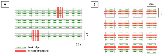
Figure 1.
(A) Layout of the leek field at the experimental centre, ‘Provinciaal Proefcentrum voor de Groenteteelt Oost-Vlaanderen’ (PCG) in Kruishoutem, cultivated under normal farming conditions. Lines indicate the delineation of plots, each representing a different fungicide used in the fungicide trial of the experimental centre in Kruishoutem. PCG plots had a dimension of 2.5 by 2.6 m. The direction of measurement is perpendicular to the crop row. (B) Layout of the leek test plots at Bottelare. Direction of measurement is along the crop row. Each plot represents a site that received one of four inoculation treatments (leek rust disease, leek white tip disease, both diseases, no disease). Results for white tip disease are not shown in this work. Bottelare plots had dimensions of 3 by 3 m.

Table 1.
Measurement scheme of the PCG and Bottelare data acquisition campaigns. Each ‘plot’ contained 4 rows of leek, but only the middle 2 rows were measured to avoid edge effects.
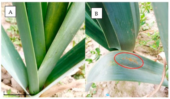
Figure 2.
(A) Healthy leek crop with 0% leaf area infected. (B) leek plant infected with rust disease, showing orange pustules on approximately 3% of leaf area infected. Scale in cm.
2.2. Visual Assessment of Rust Disease Severity
During the first measurement campaign at PCG, 6 sites were selected in the crop row for scanning based on the visual presence of rust disease. During the second scanning campaign, the same 6 sites were scanned again (Table 1; Figure 1). The average infection was measured over 25 plants for both plots, using the percentage of area covered with rust symptoms per plant as a measure for disease intensity, which conforms with the EPPO PP 1/120(2)—Guideline for the efficacy evaluation of fungicides on foliage diseases of Allium crops. The intensity of infection was only available from the experimental centre for the first measurement day in December. The first plot contained low rust infection with an average of 0.84% of the leaf area infected, while the second plot showed high rust infection, with an average of 10.32%. This gave two datasets, one with relatively low disease pressure and one with high disease pressure.
Since the Bottelare test plots showed very low levels of infection, a different disease severity assessment was used, based on the methodology described in Clarkson et al. (1997) [19]. The low amount of pustules per plant measured at the Bottelare experimental facility were likely due to the weather, which was extremely dry for the time of year, limiting spread of infection [8]. The data gathered at the Bottelare experimental farm contained mostly plants with zero rust pustules and a small amount of plants with 0–10 rust pustules per plant on average, representing an early stage of leek rust infection.
2.3. Sensor Setup
Measurements were performed with a hyperspectral pushbroom sensor with a range of 400 to 1000 nm (Specim, Oulu, Finland) and a full width at half maximum value of 5.5 nm, which is the distance between the centre and the edge of the band. Data was collected following a previously determined optimal scanning configuration, with an exposure time of 1 ms, a measurement height of 0.30 m, and a scanning angle of 17° [39]. The sensor was moved over the crop canopy with a customised aluminium frame (Figure 3). The aluminium frame formed an upturned U-shaped structure, which rested on four wheels. Between the supports of the frame, an aluminium bar with a length of 3 m was positioned at adjustable height. The sensor box was attached to this bar by a wheels-and-rail system. The aluminium frame pieces and the aluminium bar could be dismounted and broken up into several smaller pieces for transport. An electric motor powered by a 12 V battery moved the sensor box along the length of the bar at a pre-set constant speed, using a rubber driver belt. Two 500 W tungsten halogen lamps (Powerplus, Ah Joure, The Netherlands) were attached on both sides of the sensor box to provide additional illumination for the hyperspectral camera, following the setup of Whetton et al. (2018) [35]. It was essential that these lamps were halogen, to ensure they emitted radiation with a continuous spectrum [3]. A generator was used to power the sensor and artificial lamps. A battery-powered pyranometer (Skye Instruments, Llandrindod Wells, UK) was used to measure incoming solar radiation. Two reference values, a ‘dark’ reference and a ‘white’ or ‘bright’ reference, were measured at the start of each measurement, and repeatedly during measurements if the incoming solar radiation (measured with the pyranometer) varied more than 75 W/m2. The value of 75 W/m2 was empirically observed to be greater than the natural fluctuations of incident light when cloud conditions remained stable. The dark reference was the signal measured while the camera shutter or lens cap was closed, representing the background signal caused by electrical currents in the sensor. The white reference value was measured by scanning a white reference target (SphereOptics, Germany, Alucore reflectance target, 500 × 500 mm, 95% reflectance, calibrated) with the hyperspectral camera. All data storage was done on external solid state drives.
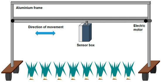
Figure 3.
Aluminium measurement frame with sensor box containing a pushbroom hyperspectral sensor, which is propelled by an electric motor at constant speeds over a lateral aluminium bar. The entire frame is then moved to measurement sites, over the crop row.
2.4. Hyperspectral Library Building
Since the pixel resolution was on the sub-millimetre scale, it was possible to visually select representative regions of interest (ROI) from hyperspectral images (belonging to both the PCG and Bottelare datasets) for each of the four classes (healthy, rust, weeds, soil), using ENVI software (Harris Geospatial, Boulder, CO, USA). Images were selected based on the clear visual presence of pure pixels for each of the four training classes, needed for ROI delineation. Each ROI consisted of an area of image pixels (spatial resolution 0.38 mm) with underlying spectra. This selection was done manually in ENVI, with the mouse button, defining the regions in the image that were clearly visible as soil, healthy leek, rust disease or weeds. The spectra belonging to these pixels were then exported from ENVI to the final hyperspectral training library (in ‘.csv’ format). This method of extracting spectra from a ROI and treating each spectrum as a sample is concurrent to the work of Xie et al. (2015), where hyperspectral data was used to detect early and late blight disease on tomato leaves [40]. The dataset resulting from these visually selected regions is referred to as the hyperspectral library.
Since the Bottelare dataset contained relatively few infection sites that were clearly visible to the naked eye on the hyperspectral images, the hyperspectral library was based solely on rust spectra measured at PCG (Table 2). More than 10,000 spectra were selected that clearly belonged to rust pustules, both shaded and unshaded. For healthy leek spectra, it was decided to only incorporate the Bottelare dataset, since it was impossible to clearly delineate fully healthy ROIs in the hyperspectral images measured at PCG, because the infection was so severe. ROIs were selected from different leaves of different plants until again more than 10,000 healthy spectra were gathered. Because the PCG dataset showed extremely low weed presence, only weed spectra from the Bottelare dataset were incorporated in the hyperspectral library. Here, weed pressure was extremely high, with dozens of weed species on the crop ridge. Again, more than 10,000 weed spectra were selected and incorporated into the hyperspectral library. These spectra were obtained from pixels that were evenly spread over the weed mass present in a representative scan taken before disease pressure was present in the field. Because weed coverage was so intense in Bottelare, it was difficult to clearly delineate ROIs that contained only soil and no plant matter with relative certainty. It was therefore necessary to select and incorporate soil spectra based on the PCG measurements. The size of each individual ROI varied, from 2 by 2 pixels for individual leek rust symptoms to several dozens by dozens of pixels for soil, healthy leek, and weeds. However, the final number of training spectra for each training class was made identical at 10,854, leading to a hyperspectral library containing 43,416 spectra.
Table 2.
Sampling location of the regions of interest used in the construction of the hyperspectral library, for each of the four classes.
2.5. Preprocessing and Model Selection
The hyperspectral library was used to optimize preprocessing and modelling, following the flow outlined in Figure 4. The square box with marked ‘Final workflow’ outlines the final workflow for detecting leek rust disease, including the steps: preprocessing 1, soil model, differentiation non-soil from soil pixels in the hyperspectral image, preprocessing 2, and finally the rust model that determines the pixels representing leek rust diseased areas of the crop. The steps that are not outlined in this box represent the steps taken to achieve the final workflow, including the following steps: initial preprocessing, data exploration, followed by an iteration of: selection of disease detection models, their evaluation on unlabelled data, and improved preprocessing. First, the process used to determine the final workflow is discussed in this section. Then, the final workflow is summarized in the next section.
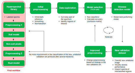
Figure 4.
Preprocessing and model selection cycle. The area highlighted in the leftmost square box with wording ‘Final workflow’ represents the final workflow. The rest of the chart represents the steps taken to determine this final workflow.
The first part of the initial preprocessing step was the pixel per pixel correction of the raw hyperspectral image from the sensor using following formula:
where R_cor is the corrected reflectance spectrum of the measured sample at a certain pixel, R_wr is the averaged white reference reflectance spectrum, representing the ‘maximum’ reflectance spectrum, measured on a calibrated white reference target (SphereOptics, Herrsching, Germany, Alucore reflectance target, 500 × 500 mm, 95% reflectance, calibrated), R_raw is the raw reflectance of the sample measured and R_dr is the averaged dark, or minimum, reflectance spectrum, measured with a closed camera shutter.
R_cor = (R_raw − R_dr)/(R_wr − R_dr)
Initial results showed that there was a lot of noise and variability in the spectral dataset. The second step therefore was to apply a Savitsky-Golay smoothing algorithm (window 33, polyorder 2), followed by a min/max normalisation that scaled the reflectance measurements between 0 and 1 [41]. The smoothing window was determined by trial and error, by iteratively changing the smoothing window from 1 to 55 (after which a greater window had no further effect) and assessing the classification accuracy. Part of the spectrum before 445 nm and after 914 nm were cut from the dataset because they appeared to contain more noise than the rest of the spectrum during data exploration (Figure 5). The presence of noise is a common issue in hyperspectral sensing, especially in field conditions, and can be caused by a variety of environmental and sensor-specific parameters [42]. Data exploration further involved the visual identification of regions in the spectrum that appeared to contain differences between the four classes of the model (healthy leek, rust disease, weeds, and soil).
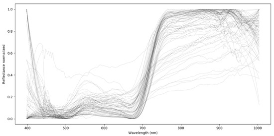
Figure 5.
Random selection of spectra from the hyperspectral library after Savitsky-Golay smoothing and normalisation, showing high amounts of noise at the beginning and end of the spectrum.
These initial preprocessed spectra (after white/dark reference correction, smoothing and normalisation) were then tested for classification using the scikit-learn library of the Python programming environment (Python Software Foundation, Wilmington, DE, USA), with a selection of common classifiers, including: K nearest neighbors classifier, support vector machine classifier, gaussian process classifier, decision tree classifier, random forest classifier, multilinear perceptron classifier, AdaBoost classifier, gaussianNB classifier, logistic regression classifier, Linear Discriminant Analysis classification, and quadratic discriminant analysis classification [43]. The classifiers were tested with both the default model parameters and variations concerning for example kernel or solver type.
To assess the performance of each classifier, the hyperspectral library was split into two datasets: 70% of the data was used for model training, and 30% was used as an independent validation set, also known as the ‘hold-out’ set [44]. The quality of this validation was assessed by computing the accuracy of classification (obtained from the confusion matrix) on the labelled validation set. The best performing model, or models in case results were close, was retained and used to classify a new, unlabelled hyperspectral image, referred to as the ‘new validation set’ in the workflow of Figure 4. The quality of this classification was then assessed by visually comparing the RGB image obtained from the hypercube to the classified image. The spectra of misclassified areas were studied, and the preprocessing or modelling strategy was adapted based on these misclassifications. These adaptations included combinations of several commonly used techniques [45,46,47,48,49]:
- Changing the wavebands used as model input based on (a) manual selection of wavebands and (b) applying wavelength selection algorithms
- Changing the smoothing window
- Changing and combining classifiers
- Including first and/or second derivative data in the model input
- Including ratios and indices in the model input
- Performing principle component analysis (PCA) and/or linear discriminant analysis as a dimensionality reduction step
- Training label manipulation by changing labels in the hyperspectral library of problematic spectra, intentionally feeding ‘falsely’ labelled data to the model to increase model performance (see Section 2.6, Final Disease Detection Workflow) [49]
After changing the preprocessing strategy following the steps mentioned above, the cycle started anew by running each classifier with this new preprocessing strategy and again calculating the accuracy. During this iterative process, some classifiers were excluded from the analysis because they consistently underperformed. This process was repeated until no apparent improvement was observed in the confusion matrix and in the unlabelled classification.
The waveband selection algorithms tested were the standard algorithms provided by the scikit-learn package, namely ‘SelectKBest’ and ‘SelectFromModel’ [43]. These algorithms suffered from the high correlation between neighbouring bands and often resulted in the selection of a group of neighbouring bands from a single spectral region as being ‘optimal’. This might not represent the true optimal combination, since it does not contain information for each region. We therefore adopted a strategy to use these waveband selection algorithms to select the optimal waveband per region of the spectrum. This then lead for example to 1 band for the first 10 bands measured, and another for each consecutive group of 10 bands. Then, the waveband selection algorithm was run again on this new group of 17 ‘optimal’ bands, resulting in a small group of 3–5 bands. Other dimensionality reduction strategies were tested as well, including LDA and PCA.
2.6. Final Disease Detection Workflow
The final workflow consisted of two classification steps: soil classification and leek rust disease classification. These two classification steps each have respective preprocessing steps, represented by ‘Preprocessing 1’ and ‘Preprocessing 2’ in Figure 4.
Preprocessing 1. First, white/dark reference correction was performed on the raw data coming from the hyperspectral camera. A Savitsky-Golay smoothing algorithm (window 33, polyorder 2) was then applied to this data. Then, reflectance values for wavelengths below 445 or higher than 914 nm were cut, retaining only the 174 bands in between. Finally, the first derivative of the reflectance curve was taken.
Soil classification model. Soil classification was achieved by using the value of the 702 nm waveband of this ‘first derivative spectrum’, combined with a standard LDA algorithm from the scikit-learn Python library. No normalisation was applied to this data during this step. This resulted in a matrix containing the location of soil and non-soil pixels. The non-soil pixel indices were then used to isolate non-soil spectra from the (non-preprocessed) hyperspectral library, which were then submitted to the ‘Preprocessing 2’ step. Note that the non-soil spectra were extracted from the non-preprocessed hyperspectral library, meaning that the spectra used in the disease detection model only received the ‘Preprocessing 2’ treatment at the time they are used as model inputs. The ‘Preprocessing 1’ and ‘Soil model’ steps were used exclusively to differentiate between soil and non-soil pixels.
Preprocessing 2. First, white/dark reference correction was performed on the raw data acquired by the hyperspectral camera. A Savitsky-Golay smoothing algorithm (window 33, polyorder 2) was then applied to this data. Then, reflectance values before 445 and after 914 nm were cut, retaining only the 174 bands in between. A normalisation step was added after this, transforming the data to a range between 0 and 1, to reduce effects of within crop shading and differences due to solar radiation. The first derivative was also taken, but after normalisation (contrary to the ‘Preprocessing 1’ step for soil classification, where the first derivative was taken before normalisation because the distinction between soil and non-soil first derivative spectra was more clear prior to normalisation). The normalisation step was necessary to reduce effects of differences in absolute reflectance, such as within crop shading. Using this data, a large amount of false positives occurred due to the misclassification of weed spectra as ‘rust’, even in scans without rust disease present in the field. Analysis of these misclassified spectra showed that these weed spectra showed a relatively high reflectance in and near the 661 nm band (reflectance of up to 0.1 after preprocessing). Rust spectra typically show a much higher reflectance in this band, up to 0.35, which is not surprising given the orange/red appearance of rust pustules. However, some rust spectra in the hyperspectral library showed a reflectance in this band lower than 0.1, making these spectra more similar to the misclassified weed spectra. It is possible that these particular rust spectra were selected (during the construction of the hyperspectral library, see Section 2.4, Hyperspectral Library Building) from pixels located at the edge of the rust pustule, where the rust spectrum is mixed with that of the surrounding plant tissue. It appeared that the similarity between certain rust spectra in the training data with relatively low reflectance (for being rust spectra) in the 661 nm band and certain weed spectra in the training data with relatively high reflectance (for being weed spectra) in the 661 nm band contributed to misclassification.
To solve this issue, the training labels of rust spectra in the hyperspectral library with a reflection in the 661 nm waveband lower than 0.13 (after preprocessing) were changed from ‘rust’ to ‘weed’, essentially performing a form of training label manipulation by intentionally feeding altered information to the training step of the model to increase model performance [49]. By changing the labels from ‘rust’ to ‘weed’ of these specific rust spectra with low reflectance in the 661 nm band, a new training dataset was created, where all rust-labelled spectra have a reflectance in the 661 nm higher than 0.13. As a result, the model learned that spectra with low reflectance in this waveband (below 0.13) should be classified as ‘non-rust spectra’, since all training spectra with a ‘rust’ label showed high reflectance (above 0.13) in this waveband. This step solved the misclassification issue and proved essential to increase model performance.
Rust classification model. The preprocessed dataset was fed to a logistic regression model using only three values: the reflectance values at 556 and 661 nm, combined with the value of the first derivative at 511 nm (see Results section for feature selection process). The class weights were set to 0.4 for rust, 1 for healthy plant parts, and 1 for weeds. The general form of a linear logistic regression model and further details on its structure can be found in the Scikit-learn documentation and in Serneels and Lambin (2001) [43,50].
3. Results
3.1. Data Exploration
Figure 6 shows a plot of the average reflectance spectrum for each of the four classes in the training dataset after normalisation and smoothing. Error bars represent the standard deviation for each wavelength. It can be observed that the healthy leek spectra appeared most ‘stable’, showing lower standard deviation values throughout the spectrum. Note that the minimum was around the 680 nm wavelength, which represents the photosystem II absorption band, which typically shows low reflectance (i.e. high absorbance) in healthy crops [51]. Weed spectra generally showed higher standard deviations, with also low reflection around the 680 nm band but with a larger standard deviation compared to the healthy leek spectra. It is interesting to note the apparent decrease in reflection at wavelengths higher than 880 nm in the weed spectrum. The difference is relatively small however, with a quite high standard deviation in this region. The rust spectrum showed both a high reflectance and a high standard deviation around the 680 nm waveband. Higher reflection in the entire red colour region of the spectrum was clearly visible, even though standard deviation values were high. It is worth noting that the red edge region appeared to start around 680–690 nm. This work therefore adopts the spectral range nomenclature proposed by Malacara (2003), but makes the distinction that the red region is defined from 625 to 690 nm and the red edge region from 690 to 750 nm [52]. The soil reflectance curve appeared more flattened compared to that of the leek, rust, and weed spectra, with less of a steep curve in the red edge region of the spectrum. The 480 nm absorption band (associated with carotenoids in leaves and soil) and the 670 nm chlorophyll absorption band showed clear minima in both the weed and healthy reflectance curves, which is in line with observation by other scientists [53]. The rust and soil reflectance curves showed no minimum at the chlorophyll band, only at the 480 nm band.
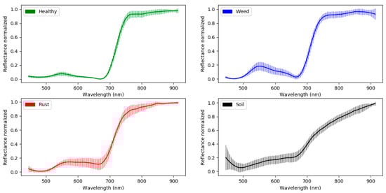
Figure 6.
Average reflectance curve for each of the four data classes included in the hyperspectral training library, after preprocessing. Error bars show standard deviation, giving an indication of the variability of the data per waveband and per class.
To compare the shape of the spectra of each of the four classes, the average reflectance curves from Figure 6 were plotted in one figure (Figure 7). The first important region to examine is the red edge region. The healthy leek spectrum showed relatively low reflectance in the visible region compared to the NIR region, resulting in a large ‘jump’ from the visible to the NIR part of the spectrum. This difference was less pronounced in the spectrum of the weed class, and even less in that of the rust class. The soil class showed an almost continuous incline, which is typical of soil, with only a mild rise in reflectance near the red edge [54]. Comparing the rest of the spectrum, there was little difference after preprocessing in the NIR region between all non-soil classes. The visible region seemed most likely to result in good classification performance, especially the spectral range between 450 and 680 nm, based on visible differences.
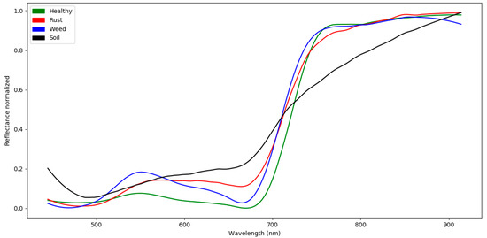
Figure 7.
Comparative plot of the average reflectance spectra of each data class of the hyperspectral training library, after normalisation and initial preprocessing steps.
3.2. Preprocessing and Model Selection
3.2.1. Preprocessing
Of the preprocessing steps listed in the materials and methods section, the following steps proved to have negligible effect on classification accuracy:
- Feature selection: feature selection algorithms did not yield better modelling results, due to the high correlation between neighbouring bands. However, the adapted feature selection strategy where the algorithm was used to select the best waveband for each region of the spectrum, and then the best wavebands overall, also did not yield better results than visual waveband selection based on the spectra in Figure 5 and Figure 6.
- Changing the smoothing window: the smoothing window was important, but did not greatly affect model performance within a given range. During the iterations of the preprocessing optimization (Figure 4), it became clear that any change in smoothing window within the range of 21 to 55 did not greatly alter the classification results.
- Including ratios and indices in the model input: several indices were tested, including normalized difference vegetation index, the red edge position index and variations on the ratio vegetation index [55,56]. None of these indices seemed to significantly improve model classification compared to the use of single wavebands, even when these indices were combined with other indices or with individual wavebands.
- Performing PCA and/or LDA as a dimensionality reduction step.
The steps that were effective for increasing model performance include:
- Changing the wavebands used as model input based on manual selection of wavebands.
- Including first and/or second derivative data in the model input.
- Training label manipulation by changing labels in the hyperspectral library of problematic spectra, intentionally feeding ‘falsely’ labelled data to the model.
- Changing and combining classifiers.
Due to the high correlation of neighbouring bands, traditional feature selection methods did not prove useful. An effort was made to counteract this correlation issue by using such feature selection on each region of the spectrum separately (e.g. for each consecutive 10 bands, determine the most important band, and then out of the resulting 17 bands determine the best 3–5 bands, see Section 2.5). It was observed that these methods did not outperform visual waveband selection based on the plots of the spectral signatures (Figure 7). The most effective waveband selection tool for increasing model performance proved to be the plotting of spectra belonging to misclassified pixels, and observing differences between those spectra and the target spectra. The addition of certain bands of the first derivative spectrum using this strategy also benefited classification. During the iterations, the number of wavebands used in the model was varied from only one or two bands to the full 348 band spectrum, which is the normal spectrum followed by the first derivative. It became clear that too many wavebands (more than 10), containing redundant information, deteriorated classification, while too little information (less than 3 wavebands) was not enough to accurately classify the data (assed using confusion matrix calculation). Furthermore, changing the label of certain input spectra was essential to achieve accurate classification of leek rust disease. The combination of two classifiers, one for soil and one for leek rust disease also greatly improved classification accuracy. From this point on, we therefore distinguish between the soil classification model and the crop classification model.
3.2.2. Model Diagnostics
Soil classification model. Soil classification was achieved with a linear discriminant analysis model, using the value of the first derivative spectrum in the 702 nm band. As seen in Figure 8, the first derivative value of the 702 nm band was 10 times smaller for soil samples compared to the other classes. The accuracy of classification was assessed using 30% of the dataset that was set aside for independent validation, with a corresponding confusion matrix shown in Table 3. A classification accuracy of 94.3% was achieved. However, it is important to note that all soil spectra were correctly classified, with a true positive rate of 1 and a subsequent false negative rate of 0. The 5.7% accuracy loss was due to misclassification of non-soil spectra. The false positive rate was low, at 7.5%, with a subsequent true negative rate of 92.4%, meaning less than 8% of the non-soil samples were misclassified as being soil. Note that the total amount of rust labelled samples in this dataset appears relatively low, while the amount of weed labelled samples appears relatively high. This is the result of the training label manipulation step, in which certain rust spectra were re-labelled as ‘weed’ (see Materials and Methods).
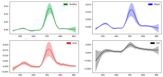
Figure 8.
First derivative of the average reflectance spectrum, after preprocessing, shown for each of the classes included in the hyperspectral training library. Error bars indicate standard deviation of the values of the first derivative, per waveband and per class.
Table 3.
Confusion matrix corresponding to the soil classification model. This model used a linear discriminant analysis classifier trained on the value of the first derivative spectrum at the 702 nm band, of the hyperspectral library (see the Section 2.4). The hyperspectral library was randomly split with a 70/30 ratio for training/validation. Columns represent the actual condition in the population (R). Rows represent the condition predicted by the model (P).
Leek rust classification model. As discussed in the methodology section, leek rust classification was achieved using the reflectance values at 556 and 661 nm, combined with the value of the first derivative at 511 nm in a logistic regression model. The results of the confusion matrix calculations are shown in Table 4. Precision and accuracy of leek rust disease classification were 99% and 98.1%, respectively. The true positive rate was 84.4%, with a subsequent false negative rate of 15.6%, meaning 84.4% of condition positives were correctly classified. The true negative rate was 99.9%, with a subsequent false positive rate of 0.1%, meaning 99.9% of the negative condition was correctly classified.
Table 4.
Confusion matrix with corresponding indices for the leek rust detection model. This model used a logistic regression classifier trained the hyperspectral library (see the Section 2.4), using the reflectance value at 556 and 661 nm, combined with the value of the first derivative at 511 nm. The class weights were set to 0.4 for rust, 1 for healthy and 1 for weeds. The hyperspectral library was randomly split with a 70/30 ratio for training/validation. Columns represent the actual condition in the population (R). Rows represent the condition predicted by the model (P).
3.2.3. Classification of Unlabelled Data
Results of the unlabelled classification still showed some misclassification of weeds in certain situations, even after the training label manipulation step described in the Materials and Methods section. Figure 9 shows a selection of these misclassified (false positive) weed spectra in green, together with rust spectra of confirmed rust pixels (red) and spectra of correctly classified weed spectra (blue). Both the green and blue spectra were selected from the leaves of one grassy weed plant, with one leaf that was classified correctly and one that was classified as a false positive. It is clear that some weed spectra (green) deviated strongly from the normal weed spectrum (blue), causing misclassification.
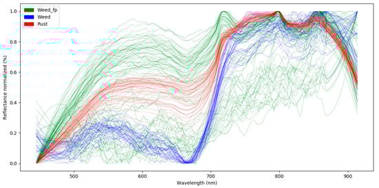
Figure 9.
Example of reflectance spectra of rust pixels (red), correctly classified weed pixels (blue) and weed pixels, which were misclassified by the rust disease classification model as rust (false positives—green).
Two representative images of these unlabelled classifications are shown in Figure 10 and Figure 11. Figure 10 shows the classification of an image from the PCG dataset, measured in February, at a different growing stage and different weather conditions compared to the data used for model building. This image contains leek plants with relatively high rust infection, but low weed pressure. Figure 10A. shows the RGB image, with circles indicating the areas magnified in Figure 10C,D, and an area containing weed pixels (rectangle) that were misclassified as rust disease. Figure 10C,D show a close-up of an area with clear rust symptoms in RGB (Figure 10D) and the classified image (Figure 10C).
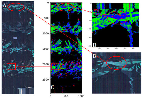
Figure 10.
Classification of a new, unlabelled validation dataset using the soil and leek rust classification models. RGB images shown (A,D) corresponding to the full classified image (B) and a close-up (C). Circles indicate a typical rust infected leaf. Rectangle corresponds to a weed plant that appeared to contain rust disease after classification.
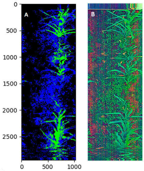
Figure 11.
Classification of a new, unlabelled validation dataset using the soil and leek rust classi-fication models. The infection score for this image is zero, an indication that no (or negligible) rust infection was present. Black pixels represent the soil, green represents healthy leek, and blue pixels represent weeds. (A) classified image and (B) RGB image taken from the hyperspectral datacube.
Figure 11 shows a representative scan for the Bottelare dataset, measured 43 days after the initial infection. It is representative of the Bottelare measurements because it shows no disease scores above zero (contrary to the PCG), with high weed coverage and a different soil type. It also represents a scan taken much later in the season, on 30 April 2019, thus for different weather conditions and a different growing stage compared to the images used in model building. Figure 11A shows the classified image. Figure 11B shows an RGB image taken from the hyperspectral datacube, which has been slightly enhanced using Microsoft Office Powerpoint software (Microsoft, Redmond, WA, USA) to make it clearer. There was no rust disease visibly present in the field. However, during classification of this dataset, a large number of false positives was encountered during the initial preprocessing and model selection steps. As seen in Figure 11, the final classification workflow was able to fully avoid false positives. Note that certain areas of the leek leaf are miscoloured blue, which is the result of the rust classification model being focused on accurately detecting leek rust disease, rather than accuracy concerning weeds versus healthy leek.
4. Discussion
4.1. Measurement Setup
Comparing the leek rust disease detection protocol in this work to that of wheat rust disease reported in the literature, some key differences become apparent [29,35]. First, one of the major constraints in wheat experiments was the absence of a measurement setup that could move the hyperspectral pushbroom sensor over the crop canopy at a continuous pace. The measurement setup in the current work made it possible to measure relatively large areas of the field from a proximal distance that gives a high pixel resolution. This resulted in a dataset with the high spatial variability and large sample size normally associated with field trials, e.g. with drone equipment, while maintaining a pixel resolution normally associated with laboratory trials [3,29,35,40,44,53,57,58]. The ability to select ROIs directly from field data and build a hyperspectral library with ‘pure’ spectra for each class is important, because one of the biggest challenges in disease detection is the translation of results from lab to field scale [1,3,4]. The results shown in Figure 7 seemed promising because there appeared to be a clear difference between healthy, rust, weed and soil spectra. However, it became apparent during modelling that the variability and the noisiness of field data was high, leading to considerable misclassification (Figure 9). A downside of this method of pixel-wise classification compared to the method of using averages over all image pixels, as used in wheat rust disease, is that the averaging of spectra removes a certain amount of noise from the data [29,35]. Since non-averaged spectra were used, a more vigorous smoothing algorithm was needed to compensate for the large amount of noise of some spectra, as seen in Figure 9, where even after vigorous smoothing considerable noise remained. This type of highly variable reflectance spectra could be caused by a number of reasons, for example the overlap of different types of classes in one pixel, creating a hybrid spectrum. Another possible explanation is that due to the low exposure time of the sensor (1 ms), some areas of the crop showed very low, noisy reflectance spectra. This effect would then be magnified by the normalisation preprocessing step. The low exposure time was necessary, however, to avoid saturation under field conditions and to allow sufficiently high scanning frequency to match the speed of the electric motor sliding the hyperspectral camera over the crop canopy, so a sharp image could be produced.
Some other practical difficulties associated with field measurements include windiness, varying solar radiation due to cloud movement, rain and dust damaging the sensor setup, and higher variability in growing conditions and stresses compared to the laboratory environment. During detection of wheat rust disease (using average reflectance measurements over a certain area over the crop), this made it difficult to assess whether any change in the average reflectance curve was caused by disease or by other stress factors or different growing conditions [3]. It was therefore an important advantage to be able to visually select ROIs containing leek rust infection on field data at within-leaf spatial resolution, rather than take average values measured over several plants, because it allowed the comparison of reflectance spectra coming from non-averaged pixels belonging specifically to diseased or healthy leek tissue on the same plant/leaf.
To apply this leek rust disease detection measurement setup in practice, it could be interesting to employ multispectral sensors that specifically focus on the wavebands used by the soil and leek rust disease detection model. Then, multiple sensors could be placed on the sprayer to map the spread of disease throughout the field. This could then be used to either immediately apply variable rate spraying (if data processing occurs fast enough), to adapt future disease management strategies, or even perform selective harvesting based on disease incidence. However, the high cost for buying multiple sensors is an issue, especially if these sensors are specific for one disease. It would be a significant improvement if certain bands could be found that can be used to detect a range of diseases, increasing the profitability of each sensor.
4.2. Preprocessing and Model Selection
Results of the preprocessing optimization (Figure 4) showed that despite the clear differences in the average spectra of Figure 7, several steps were needed to achieve acceptable model performance. The first step involved the development of a dedicated soil classification model. This was necessary, because the use of strategies such as soil pixel deletion based on the Normalized Difference Vegetation Index (NDVI) proved unreliable after normalisation and Savitsky-Golay smoothing, leading to soil NDVI values of over 0.8, as opposed to values of less than 0.3 for soil spectra reported by other authors [30,58,59]. A method was developed that, to the best of our knowledge, is new for the deletion of soil spectra. Exploration of the data showed that the difference between soil spectra and rust/healthy/weed spectra was most distinct when the dataset was subjected to first order derivation and smoothing, without normalisation. Using only the 702 nm wavelength reflectance value, it was possible to correctly classify and isolate soil spectra in the validation set, leading to a true positive rate of 1 (Table 3). With a false positive rate of 0.075, only around 8% of the non-soil pixels were misclassified as soil. Given that 91% of these misclassifications were weed spectra and 9% rust spectra, the chance of rust pixels being misclassified by the soil classification model was 0.7%. Looking at the validation of a completely new, unlabelled hyperspectral image, the performance of the soil classification model was high, giving a clear separation between soil and crop pixels (Figure 10). Even the small white reference target in the centre of the image and the black plastic pot supporting it were classified as soil (or non-plant material). The bottom of the image shows a section where the hyperspectral imager scanned the edge of the aluminium plate that affixes the aluminium frame to the wheel base. In addition, these pixels were classified as soil and excluded from further analysis.
Following soil pixel classification, the remaining non-soil pixels were used to train a model dedicated to distinguishing rust disease symptoms from weeds and healthy leek crops. The goal of this model is the mapping of the spread of leek rust disease throughout the field. Given that disease typically occurs in patches, especially for windborne diseases such as rust, it is not necessary for the model to be able to detect all rust pustules on the crop. If only a certain percentage of rust spots in a certain area are detected, it is enough indication to have to apply fungicides in that area of the field because it is likely the wider area is also infected. Moreover, the economic threshold for leek rust disease is zero, meaning fungicides are to be applied whether one or fifty rust pustules are present [12]. In the context of reducing fungicide usage, it is therefore more important that rust pustules detected are effectively rust, and not a false positive, than to detect every rust pustule present, with the risk of increasing the amount of false positives. This differs from other diseases that are tolerable at mild infection rates, in which case it is important to know exactly how much infection occurs because this affects the decision to spray or not. In the case of leek rust disease, fungicides have to be applied as soon as one pustule is detected, meaning it is not necessary to know the exact number of rust pustules as long as their presence is detected with relative certainty. The focus was therefore on reducing the amount of false positives during modelling.
It was observed during model building iterations that large amounts of false positives stemmed from the misclassification of weed pixels as rust, also in images taken before disease was present in the field. To account for this problem, two extra preprocessing steps were introduced. First, training label manipulation was performed by altering the label from ‘rust to ‘weed’ of all rust training samples with a reflectance (after preprocessing) lower than 0.13 in the 661 nm band. This step greatly reduced the amount of false positives due to weed misclassification. The second step was to shift the model weights to give less weight to the rust class, and more weight to the healthy and weed classes. This further reduced the amount of weed pixel misclassification, to the point where even images with heavy weed infection showed no misclassification (Figure 11).
As seen in Table 4, the final model succeeded in avoiding a large number of false positives, even though this comes at a price of more false negatives. A true positive rate of 84.42% was achieved, meaning 84.42% of the condition positives in the population were detected (Table 4), leading to a relatively large sensitivity to detect the presence of rust disease pustules. Moreover, even though the accuracy of this model was relatively low at 84%, the precision was high at 99%. This again indicates that the model performance focuses on detecting rust disease and accurately classifying these pixels, with less importance given to the correct classification of weeds or healthy leek pixels.
In the model presented in this work, the false positive rate was 0.1%, meaning that 1 out of 1000 non-rust pixels was misclassified. This seems like an acceptably low ratio, but in field conditions, it could be a problem. Given that the sensor has a scanning width of 1024 pixels, this 1 in 1000 false positive ratio is significant. Two important remarks have to be made. First, out of these 1024 pixels, a relatively large amount will be soil pixels (depending on the growing stage). Looking at the confusion matrix of the soil classification model, not a single soil pixel was misclassified as rust (Table 3). Secondly, the 1/1000 false positive ratio is most problematic if the false positives appear randomly. Looking at Figure 9, Figure 10 and Figure 11, it is clear that the false positive values did not appear randomly. Specific weed or healthy leek spectra were misclassified as rust, based on their reflectance spectrum (Figure 9). Moreover, the classification shown in Figure 11 shows that there is no problem of false positives appearing in approximately 3 million classified pixels.
In the final model, the largest amount of misclassifications came from misclassifying healthy plant pixels as ‘weed’ (Figure 10 and Figure 11). It makes sense that spectra of healthy leek crops and healthy weed plants appear more similar and require models that specialize in making this distinction (which is not the purpose of this study). However, as seen in the square at the bottom of Figure 10, there were also some incidents of false rust detection due to misclassification of weed pixels. The spectra in Figure 9 show that these persistently misclassified weed spectra (green) strongly deviate from the normal weed spectrum (blue). We can further see that there is a similarity between the reflectance spectra of misclassified weeds and rust pustules (red). Both curves show an elevation in the amount of reflectance measured in the red region of the spectrum, which is typical of fully developed rust pustules. It could be possible that there is an effect due to low reflectance or shading, causing a low intensity signal in the sensor that gives a distorted spectrum after normalisation. However, the fact that both the correctly classified (blue) and the misclassified (green) spectra were obtained from the same plant does not support this assumption. Another possible explanation is that the misclassified weeds were infected either by rust disease or another pathogen or stress factor, leading to spectra similar to rust disease spectra on leek. This assumption is supported by the fact that this type of misclassification was only observed on hyperspectral images of leek rows showing a high degree of rust infection (Figure 10), and not on images taken before rust disease was present in the crop (Figure 11). Looking at Figure 11, there are no false positives, even though there is ample weed cover, with certain areas showing low reflectance signals due to for example the angle between the sensor and the weed leaf. This supports the assumption that these misclassified spectra indicate rust disease or a different stress in the weed plant, rather than being caused by the measurement conditions or random noise.
Note that due to the lateral movement of the hyperspectral sensor during measurement, there was a distortion (wobble-effect) in the hyperspectral image. However, due to the fact that the data analysis uses spectral information on a pixel-by-pixel basis (rather than on a full plant level), this did not affect data analysis. The presence of vertical stripe noise, which is typical for pushbroom hyperspectral sensors [60], also did not affect the classification in these bands (Figure 10 and Figure 11).
Due to the focus on a low number of false positives, the amount of rust pustules missed during classification increased. In practice, this would mean that the farmer would falsely assume an area of the field is infected and waste fungicides, leading to an increased cost and a pressure on the environment. It is therefore necessary to further research the trade-off between (a) the risk of missing an infected area when the model focus is on reducing false positives, and (b) wasting more fungicides on an increased number false positives, when the focus is on missing as few rust pustules as possible. As stated before, the economic threshold for rust disease is essentially zero, meaning fungicides are applied even at low infection rates due to cosmetic damage. Looking at the confusion matrix (Table 4), the leek rust detection model showed a miss rate of only 15.6%. This means that there is a roughly one in six chance of not detecting a rust pixel, which is relatively low for practical purposes given that as soon as one rust pixel is detected, the immediate surrounding area is treated with fungicides. This could however be an issue if the amount of linescans decreases for practical applications, leading to for example one scan every 0.10 m. The validity of this disease detection model in practice must therefore be tested under field conditions with variable rust disease pressure. Moreover, the spread of rust disease depends highly on the weather, meaning some conditions are worse for ‘missing’ an infected site compared to others. This information also needs to be taken into account for practical applications. Lastly, it needs to be tested whether the reduction in fungicides used outweighs any potentially missed infection sites, which in turn spread infection to the rest of the field.
4.3. Optimal Wavebands for Detecting Leek Rust Disease
The selection of the optimal combination of features is important to remove wavebands with low discriminative power between classes from model training, thus increasing model performance [54]. The optimum waveband combination for leek rust disease detection consisted of 1 band at 702 nm for the soil classification model and three bands, namely the 556 and 661 nm band, combined with the value of the first derivative at 511 nm, for the disease classification model. The 702 band lies at the start of the red edge region, which signifies the ‘jump’ in the reflectance curve typically seen in plant spectra (where chlorophyll absorption takes place), but not as prominently in soil spectra (Figure 7). The 511 nm band lies in the cyan colour part of the spectrum, the 556nm band in the green part, and 661 nm band in the red part [52]. This result is not surprising, given that leek leaves are normally blue-greenish in colour, while rust pustules appear a bright orange-red. It is important to note that three bands is a relatively low amount of wavebands to include in a rust detection model, compared to a recent study reporting six selected bands for wheat rust detection [29]. These researchers found the 538, 598, 689, 702, 751, and 895 nm bands to be optimal for detection of wheat rust disease, highlighting the importance of the visual region, which includes all of the bands used in the leek rust detection model presented in this work, but also of the NIR region. The importance of the visual region of the spectrum for rust detection on wheat has already been suggested in 2004 by Moshou et al. [34], and has later been confirmed by numerous authors for rust disease of wheat and sugarcane, and for other diseases such as Fusarium disease on wheat [31,35,61,62]. It can be noted that contrary to the results found for leek rust disease, many of the authors above included the NIR region into their rust disease model. The addition of NIR bands was found to not increase model performance compared to the current rust disease detection model setup. However, as indicated by other authors, this region also contains discriminative information and could be used in addition to the information presented in the visible region, if needed. It can be further observed that in all studies mentioned above, no two works conclude on the same optimal waveband selection. It is for this reason that authors often mention optimal waveband ranges, since there is a large correlation between neighbouring bands when the spectral resolution of the sensor is high enough. This was also observed during model training, where waveband selection algorithms often resulted in the selection of a group of directly adjacent bands as being ‘optimal’. The fact that a relatively simple logistic regression model (compared to more complex deep learning structures) with relatively few bands could be used to detect the pathogen is beneficial for practical applications. This because it is less challenging to implement these models in small processors on farm equipment, and the low number of bands suggest it might be possible to replace the hyperspectral sensor with cheaper, easier to use sensors (RGB, multispectral).
4.4. Challenges and Future Perspective
As mentioned in the introduction, three key problems remain in close-range hyperspectral imaging under field conditions: (a) the variability of reflectance due to within-crop shading and the complex geometry of the crop canopy, (b) the extremely large amount of data provided by these techniques, and (c) the high cost of commercially available hyperspectral sensors [38]. The latter can partially be addressed by the fact that more and more researchers are using these sensors, increasing demand and therefore production, which is gradually decreasing prices. Additionally, the fact that only a few wavebands were needed for leek rust disease detection gives the opportunity to replace the expensive hyperspectral sensor with a much cheaper multispectral sensor that is dedicated to measuring these specific wavebands.
As shown in Figure 10, the disease detection model suffers from the problem of a complex reflectance pattern caused by the crop canopy structure and within-crop shading, leading to a misclassification of weeds and healthy crops. Even after normalisation, this issue could not be resolved. However, this problem did not affect the ability of the model to detect rust symptoms. Even in the shaded areas of the crop canopy, the classification of rust disease is accurate to a pixel level. The ability to detect single rust pustules opens up possibilities for variable rate fungicide applications, since it is suggested in the literature that it is possible to curatively treat early rust infection [10].
Another problem of close-range hyperspectral imaging is the large amount of data to be processed. If this model is to be used in variable rate applications, a sufficiently high sampling density needs to be achieved to ensure the detection of any disease present with high enough certainty. The mapping of an entire field would require storage capacity easily exceeding the terabyte level, even for small fields. To solve this issue, two possible modes of action are proposed. First, reducing the sampling resolution, either by increasing pixel size (measuring from a greater altitude), or by reducing the amount of lines scanned per m2 of the crop. An increase in altitude would mean that pixel size increases to be larger than individual rust pustules, which could greatly decrease disease detection potential. However, a greater measuring height also increases the width of the scanned area, so that fewer scans are needed to map a certain area. In this work, a scanning height of 0.30 m resulted in a sub-millimetre pixel size, while maintaining a scanning width larger than the width of the canopy of a single leek row. The reduction of the amount of samples per m2 would also increase the chance of missing an infected area of the crop canopy. This reduction can be divided into two options: (a) reducing the amount of lines scanned in the field, where one line consists of a measurement across the entire length of the field, and (b) reducing the amount of samples taken per line scanned. Future experiments have to clarify to which extent either of these options are viable, and what the optimal sampling resolution and distribution is.
Besides the issue of data storage, another important downside of map-based variable rate fungicide applications is the increase in time and fuel needed to first scan the field, then produce maps, and finally return to the field to apply fungicides. This cost could outweigh the gains achieved by variable rate fungicide treatments. A possible solution for this problem would be to use a faster, less fuel intensive vehicle (rover, robot or drone) to produce a disease map. Another strategy to reduce fuel use could be immediate, real-time processing of sensor data measured on the front of a sprayer, directly followed by variable rate fungicide application at the back. This could for example be done with multiple cheaper, multispectral sensors specifically aimed at the wavebands needed for the model. If the sensor signal is immediately processed and this result (diseased or not diseased) is immediately sent to a sprayer, there is no need for data storage, as sensor-based variable rate application can be implemented. However, this would require high computing power and multiple sensors, mounted far enough in front of the spray nozzles to allow time for computation. The speed at which the sprayer could be driven would then depend on both the desired sampling density and the speed at which the signal can be processed. If this means the vehicle needs to move at a low velocity, the fuel and labour costs of the operation could again outweigh the benefits of variable rate fungicide treatments. A possible solution would be the combination of disease detection with other cultivation practices such as weeding. Note that also for these automated (non-map based) methods, it could be useful to map the spread of disease in the field for later use. An important downside of these specialised multispectral sensors would be that they are focused on just one disease. It would therefore be interesting to test whether certain combinations of wavebands can be used to detect more than one disease.
Based on literature on wheat rust detection, the most promising method for variable rate leek rust treatment could be the use of a mapping method but with a lower sample resolution (for example one sample per 0.10 m) [3]. However, the canopy structure in wheat is much more uniform compared to leek. This makes it more likely for a single line to contain relatively large amounts of soil pixels in scans of a leek canopy compared to a wheat canopy, which is denser. Additionally, the difference in canopy structure could potentially mean that rust symptoms are more easily concealed in lower parts of the leek canopy. Dedicated experiments in leek crops are therefore needed to validate this methodology used in wheat [3].
5. Conclusions
Based on the hyperspectral sensing experiments on rust disease in leek canopies carried out in two experimental sites, the developed methodology shows promising results for detection of rust pustules under field conditions. The capacity to differentiate weeds from healthy leek plants can be further improved to increase the usefulness of this system for the farmer. Further development is also necessary to integrate data acquisition and analysis in an automatic framework for immediate analyses after scanning. This would allow for sensor-based variable rate fungicide application by means of real-time on-line measurement of leek disease pressure, by setting up the hyperspectral sensor on a sprayer, followed immediately by automatic data analysis and fungicide treatment if necessary. A first step towards this goal is the scanning and mapping of an entire field and producing management zone maps. Even if it is not possible to implement sensor-based fungicides application, it would be interesting to investigate the use of disease maps for future farm management. The hypothesis that this model could be used to curatively treat rust infections should also be investigated. It would further be useful to explore the use of fast, fuel efficient modes of transportation, such as drones, to map the disease pressure in the field before fungicide application. Lastly, it could prove interesting to try to expand the methodology used in this work to a new leek disease and see if it is possible to distinguish between several diseases present in the same crop.
Author Contributions
Conceptualization, S.A., J.G.P. and A.M.M.; data curation, A.M.M.; formal analysis, S.A.; funding acquisition, A.M.M.; investigation, S.A.; methodology, S.A., J.G.P. and A.M.M.; project administration, J.G.P. and A.M.M.; resources, A.M.M.; software, S.A.; supervision, J.G.P. and A.M.M.; validation, S.A., J.G.P. and A.M.M.; visualization, S.A.; writing—original draft, S.A.; writing—review & editing, S.A., J.G.P. and A.M.M. All authors have read and agreed to the published version of the manuscript.
Funding
The author(s) disclosed receipt of the following financial support for the research, authorship, and/or publication of this article: This work was supported by the Research Foundation—Flanders (FWO) for Odysseus I SiTeMan Project [Nr. G0F9216N].
Data Availability Statement
Data available from Ghent University data server upon reasonable request.
Acknowledgments
Apart from the people listed on this paper, a big thanks to the people at Bottelare experimental farm, UGent mechanical workshop, the people from the ‘Provinciaal Proefcentrum voor de Groenteteelt Oost-Vlaanderen’, and the colleagues of our research group who helped me in the field.
Conflicts of Interest
The authors declare no conflict of interest.
References
- Bohnenkamp, D.; Behmann, J.; Mahlein, A.-K. In-Field Detection of Yellow Rust in Wheat on the Ground Canopy and UAV Scale. Remote Sens. 2019, 11, 2495. [Google Scholar] [CrossRef]
- Agrios, G. Plant Pathology, 5th ed.; Academic Press: San Diego, CA, USA, 2005. [Google Scholar] [CrossRef]
- Whetton, R.L.; Waine, T.W.; Mouazen, A.M. Hyperspectral measurements of yellow rust and fusarium head blight in cereal crops: Part 2: On-line field measurement. Biosyst. Eng. 2018, 167, 144–158. [Google Scholar] [CrossRef]
- Zhang, J.; Huang, Y.; Pu, R.; Gonzalez-Moreno, P.; Yuan, L.; Wu, K.; Huang, W. Monitoring plant diseases and pests through remote sensing technology: A review. Comput. Electron. Agric. 2019, 165, 104943. [Google Scholar] [CrossRef]
- De Clercq, H.; Peusens, D.; Roldan-Ruiz, I.; Van Bockstaele, E. Causal relationships between inbreeding, seed characteristics and plant performance in leek (Allium porrum L.). Euphytica 2003, 134, 103–115. [Google Scholar] [CrossRef]
- Smilde, W.; Van Nes, M.; Reinink, K.; Kik, C. Genetical studies of resistance to Phytophthora porri in Allium porrum, using a new early screening method. Euphytica 1997, 93, 345–352. [Google Scholar] [CrossRef]
- Declercq, B.; Van Buyten, E.; Claeys, S.; Cap, N.; De Nies, J.; Pollet, S.; Höfte, M. Molecular characterization of Phytophthora porri and closely related species and their pathogenicity on leek (Allium porrum). Eur. J. Plant Pathol. 2010, 127, 341–350. [Google Scholar] [CrossRef]
- Gilles, T.; Kennedy, R. Effects of an Interaction Between Inoculum Density and Temperature on Germination of Puccinia allii Urediniospores and Leek Rust Progress. Phytopathology 2003, 93, 413–420. [Google Scholar] [CrossRef] [PubMed]
- Bruycker, E.D.; Reyke, L.D.; Plovie, N.; Callens, D.; Roosterd, L.D.; Cardoen, I.; Delobelle, I.; Tierry, L.; van de Steene, F.; Hofte, M. Ziekten En Plagen in Prei; 2004; p. 23. [Google Scholar]
- Cap, N.; De Rooster, L.; Darwich, S. Roestbestrijding in Prei. Proeftuin Nieuws, 3 July 2014; 32–35. [Google Scholar]
- Geiger, F.; Bengtsson, J.; Berendse, F.; Weisser, W.W.; Emmerson, M.; Morales, M.B.; Ceryngier, P.; Liira, J.; Tscharntke, T.; Winqvist, C.; et al. Persistent negative effects of pesticides on biodiversity and biological control potential on European farmland. Basic Appl. Ecol. 2010, 11, 97–105. [Google Scholar] [CrossRef]
- de Jong, P.D.; Daamen, R.A.; Rabbinge, R. The reduction of chemical control of leek rust, a simulation study. Eur. J. Plant Pathol. 1995, 101, 687–693. [Google Scholar] [CrossRef][Green Version]
- Taylor, G.A.; Torres, H.B.; Ruiz, F.; Marin, M.N.; Chaves, D.M.; Arboleda, L.T.; Parra, C.; Carrillo, H.; Mouazen, A.M. pH Measurement IoT System for Precision Agriculture Applications. IEEE Lat. Am. Trans. 2019, 17, 823–832. [Google Scholar] [CrossRef]
- Mahlein, A.-K. Plant Disease Detection by Imaging Sensors—Parallels and Specific Demands for Precision Agriculture and Plant Phenotyping. Plant Dis. 2016, 100, 241–251. [Google Scholar] [CrossRef]
- Nawar, S.; Corstanje, R.; Halcro, G.; Mulla, D.; Mouazen, A.M. Delineation of Soil Management Zones for Variable-Rate Fertilization. Adv. Agron. 2017, 143, 175–245. [Google Scholar] [CrossRef]
- Behmann, J.; Mahlein, A.-K.; Rumpf, T.; Römer, C.; Plümer, L. A review of advanced machine learning methods for the detection of biotic stress in precision crop protection. Precis. Agric. 2015, 16, 239–260. [Google Scholar] [CrossRef]
- Grisham, M.P.; Johnson, R.M.; Zimba, P.V. Detecting Sugarcane yellow leaf virus infection in asymptomatic leaves with hyperspectral remote sensing and associated leaf pigment changes. J. Virol. Methods 2010, 167, 140–145. [Google Scholar] [CrossRef] [PubMed]
- Zhang, J.; Pu, R.; Huang, W.; Yuan, L.; Luo, J.; Wang, J. Using in-situ hyperspectral data for detecting and discriminating yellow rust disease from nutrient stresses. Field Crop. Res. 2012, 134, 165–174. [Google Scholar] [CrossRef]
- Clarkson, J.P.; Kennedy, R.; Phelps, K.; Davies, J.; Bowtell, J. Quantifying the effect of reduced doses of propiconazole (Tilt) and initial disease incidence on leek rust development. Plant Pathol. 1997, 46, 952–963. [Google Scholar] [CrossRef]
- De Jong, P. Disease Management of Leek Rust, a Study at Field, Farm and Regional Level. 1995. Available online: https://edepot.wur.nl/206535 (accessed on 31 March 2021).
- Doherty, M.A.; Preece, T. Bacillus cereus prevents germination of uredospores of Puccinia allii and the development of rust disease of leek, Allium porrum, in controlled environments. Physiol. Plant Pathol. 1978, 12, 123–132. [Google Scholar] [CrossRef]
- Huang, J.W. Control of Chinese Leek Rust with a Plant Nutrient Formulation. Plant Pathol. Bull. 1994, 3, 9–17. [Google Scholar]
- Jennings, D.M.; Ford-Lloyd, B.; Butler, G.M. Effect of plant age, leaf position and leaf segment on infection of leek by leek rust, Puccinia allii. Plant Pathol. 1990, 39, 591–597. [Google Scholar] [CrossRef]
- Jong, P.D.; Bree, J. Analysis of the spatial distribution of rust-infected leek plants with the Black-White join-count statistic. Eur. J. Plant Pathol. 1995, 101, 133–137. [Google Scholar] [CrossRef]
- Roberts, A.M.; Walters, D.R. Nitrogen assimilation and metabolism in rusted leek leaves. Physiol. Mol. Plant Pathol. 1988, 32, 229–235. [Google Scholar] [CrossRef]
- Roberts, A.M.; Walters, D.R. Shoot: Root interrelationships in leeks infected with the rust, Puccinia allii Rud.: Growth and nutrient relations. New Phytol. 1989, 111, 223–228. [Google Scholar] [CrossRef]
- Smith, B.M.; Crowther, T.C.; Clarkson, J.P.; Trueman, L. Partial resistance to rust (Puccinia allii) in cultivated leek (Allium ampeloprasum ssp. porrum): Estimation and improvement. Ann. Appl. Biol. 2000, 137, 43–51. [Google Scholar] [CrossRef]
- Theunissen, J.; Schelling, G. Pest and disease management by intercropping: Suppression of thrips and rust in leek. Int. J. Pest Manag. 1996, 42, 227–234. [Google Scholar] [CrossRef]
- Guo, A.; Huang, W.; Ye, H.; Dong, Y.; Ma, H.; Ren, Y.; Ruan, C. Identification of Wheat Yellow Rust Using Spectral and Texture Features of Hyperspectral Images. Remote Sens. 2020, 12, 1419. [Google Scholar] [CrossRef]
- Whetton, R.L.; Waine, T.W.; Mouazen, A.M. Optimising configuration of a hyperspectral imager for on-line field measurement of wheat canopy. Biosyst. Eng. 2017, 155, 84–95. [Google Scholar] [CrossRef]
- Apan, A.; Held, A.; Phinn, S.; Markley, J. Detecting sugarcane ‘orange rust’ disease using EO-1 Hyperion hyperspectral imagery. Int. J. Remote Sens. 2004, 25, 489–498. [Google Scholar] [CrossRef]
- Huang, W.; Lamb, D.W.; Niu, Z.; Zhang, Y.; Liu, L.; Wang, J. Identification of yellow rust in wheat using in-situ spectral reflectance measurements and airborne hyperspectral imaging. Precis. Agric. 2007, 8, 187–197. [Google Scholar] [CrossRef]
- Zhang, J.; Yuan, L.; Pu, R.; Loraamm, R.W.; Yang, G.; Wang, J. Comparison between wavelet spectral features and conventional spectral features in detecting yellow rust for winter wheat. Comput. Electron. Agric. 2014, 100, 79–87. [Google Scholar] [CrossRef]
- Moshou, D.; Bravo, C.; West, J.; Wahlen, S.; McCartney, A.; Ramon, H. Automatic detection of ‘yellow rust’ in wheat using reflectance measurements and neural networks. Comput. Electron. Agric. 2004, 44, 173–188. [Google Scholar] [CrossRef]
- Whetton, R.L.; Hassall, K.L.; Waine, T.W.; Mouazen, A.M. Hyperspectral measurements of yellow rust and fusarium head blight in cereal crops: Part 1: Laboratory study. Biosyst. Eng. 2018, 166, 101–115. [Google Scholar] [CrossRef]
- Paulus, S.; Mahlein, A.-K. Technical workflows for hyperspectral plant image assessment and processing on the greenhouse and laboratory scale. GigaScience 2020, 9. [Google Scholar] [CrossRef] [PubMed]
- Mahlein, A.-K.; Kuska, M.; Behmann, J.; Polder, G.; Walter, A. Hyperspectral Sensors and Imaging Technologies in Phytopathology: State of the Art. Annu. Rev. Phytopathol. 2018, 56, 535–558. [Google Scholar] [CrossRef]
- Mishra, P.; Asaari, M.S.M.; Herrero-Langreo, A.; Lohumi, S.; Diezma, B.; Scheunders, P. Close range hyperspectral imaging of plants: A review. Biosyst. Eng. 2017, 164, 49–67. [Google Scholar] [CrossRef]
- Appeltans, S.; Guerrero, A.; Nawar, S.; Pieters, J.; Mouazen, A. Practical Recommendations for Hyperspectral and Thermal Proximal Disease Sensing in Potato and Leek Fields. Remote. Sens. 2020, 12, 1939. [Google Scholar] [CrossRef]
- Xie, C.; Shao, Y.; Li, X.; He, Y. Detection of early blight and late blight diseases on tomato leaves using hyperspectral imaging. Sci. Rep. 2015, 5, 16564. [Google Scholar] [CrossRef]
- Virtanen, P.; Gommers, R.; Oliphant, T.E.; Haberland, M.; Reddy, T.; Cournapeau, D.; Burovski, E.; Peterson, P.; Weckesser, W.; Bright, J.; et al. SciPy 1.0: Fundamental algorithms for scientific computing in Python. Nat. Methods 2020, 17, 261–272. [Google Scholar] [CrossRef]
- Rasti, B.; Scheunders, P.; Ghamisi, P.; Licciardi, G.; Chanussot, J. Noise Reduction in Hyperspectral Imagery: Overview and Application. Remote Sens. 2018, 10, 482. [Google Scholar] [CrossRef]
- Pedregosa, F.; Varoquaux, G.; Gramfort, A.; Michel, V.; Thirion, B.; Grisel, O.; Blondel, M.; Prettenhofer, P.; Weiss, R.; Dubourg, V.; et al. Scikit-Learn: Machine Learning in Python. JMLR 2011, 12, 2825–2830. [Google Scholar]
- Abdulridha, J.; Ehsani, R.; De Castro, A. Detection and Differentiation between Laurel Wilt Disease, Phytophthora Disease, and Salinity Damage Using a Hyperspectral Sensing Technique. Agriculture 2016, 6, 56. [Google Scholar] [CrossRef]
- Rinnan, Å.; Berg, F.V.D.; Engelsen, S.B. Review of the most common pre-processing techniques for near-infrared spectra. TrAC Trends Anal. Chem. 2009, 28, 1201–1222. [Google Scholar] [CrossRef]
- Caporaso, N.; Whitworth, M.B.; Fisk, I.D. Near-Infrared spectroscopy and hyperspectral imaging for non-destructive quality assessment of cereal grains. Appl. Spectrosc. Rev. 2018, 53, 667–687. [Google Scholar] [CrossRef]
- Lowe, A.; Harrison, N.; French, A.P. Hyperspectral image analysis techniques for the detection and classification of the early onset of plant disease and stress. Plant Methods 2017, 13, 1–12. [Google Scholar] [CrossRef] [PubMed]
- Sankaran, S.; Mishra, A.; Ehsani, R.; Davis, C. A review of advanced techniques for detecting plant diseases. Comput. Electron. Agric. 2010, 72, 1–13. [Google Scholar] [CrossRef]
- Heaton, J. An Empirical Analysis of Feature Engineering for Predictive Modeling. In Proceedings of the Conference Proceedings-IEEE SOUTH-EASTCON, Norfolk, VA, USA, 30 March–3 April 2016. [Google Scholar] [CrossRef]
- Serneels, S.; Lambin, E.F. Proximate causes of land-use change in Narok District, Kenya: A spatial statistical model. Agric. Ecosyst. Environ. 2001, 85, 65–81. [Google Scholar] [CrossRef]
- Murchie, E.; Lawson, T. Chlorophyll fluorescence analysis: A guide to good practice and understanding some new applications. J. Exp. Bot. 2013, 64, 3983–3998. [Google Scholar] [CrossRef] [PubMed]
- Malacara, D. Color vision and colorimetry: Theory and applications. Color Res. Appl. 2002, 28, 77–78. [Google Scholar] [CrossRef]
- Hunt, E.R.; Doraiswamy, P.C.; McMurtrey, J.E.; Daughtry, C.S.; Perry, E.M.; Akhmedov, B. A visible band index for remote sensing leaf chlorophyll content at the canopy scale. Int. J. Appl. Earth Obs. Geoinf. 2013, 21, 103–112. [Google Scholar] [CrossRef]
- Hong, Y.; Guo, L.; Chen, S.; Linderman, M.; Mouazen, A.M.; Yu, L.; Chen, Y.; Liu, Y.; Liu, Y.; Cheng, H.; et al. Exploring the potential of airborne hyperspectral image for estimating topsoil organic carbon: Effects of fractional-order derivative and optimal band combination algorithm. Geoderma 2020, 365. [Google Scholar] [CrossRef]
- Curran, P.J.; Dungan, J.L.; Gholz, H.L. Exploring the relationship between reflectance red edge and chlorophyll content in slash pine. Tree Physiol. 1990, 7, 33–48. [Google Scholar] [CrossRef]
- Xue, J.; Su, B. Significant Remote Sensing Vegetation Indices: A Review of Developments and Applications. J. Sens. 2017, 2017, 1–17. [Google Scholar] [CrossRef]
- Sugiura, R.; Tsuda, S.; Tamiya, S.; Itoh, A.; Nishiwaki, K.; Murakami, N.; Shibuya, Y.; Hirafuji, M.; Nuske, S. Field phenotyping system for the assessment of potato late blight resistance using RGB imagery from an unmanned aerial vehicle. Biosyst. Eng. 2016, 148, 1–10. [Google Scholar] [CrossRef]
- Bravo, C.; Moshou, D.; Oberti, R.; West, J.S.; McCartney, A.; Bodria, L.; Ramon, H.; Orberti, R.; West, J.S.; McCartney, A.; et al. Foliar Disease Detection in the Field Using Optical Sensor Fusion. Agric. Eng. Int. CIGR J. 2004, VI, 8. [Google Scholar]
- Rouse, J.W.; Haas, R.H.; Schell, J.A.; Deering, D.W. Monitoring the Vernal Advancement and Retrogradation (Green Wave Effect) of Natural Vegetation. 1974; NASA/GSFC Type III Final Report, Greenbelt, Md, 371. [Google Scholar]
- Gómez-Chova, L.; Alonso, L.; Guanter, L.; Valls, G.C.-; Calpe, J.; Moreno, J. Correction of systematic spatial noise in push-broom hyperspectral sensors: Application to CHRIS/PROBA images. Appl. Opt. 2008, 47, F46–F60. [Google Scholar] [CrossRef] [PubMed]
- Bauriegel, E.; Giebel, A.; Geyer, M.; Schmidt, U.; Herppich, W. Early detection of Fusarium infection in wheat using hyper-spectral imaging. Comput. Electron. Agric. 2011, 75, 304–312. [Google Scholar] [CrossRef]
- Krishna, G.; Sahoo, R.N.; Pargal, S.; Gupta, V.K.; Sinha, P.; Bhagat, S.; Saharan, M.; Singh, R.; Chattopadhyay, C. Assessing Wheat Yellow Rust Disease through Hyperspectral Remote Sensing. Int. Arch. Photogramm. Remote Sens. Spatial Inf. Sci. 2014, XL8, 1413–1416. [Google Scholar] [CrossRef]
Publisher’s Note: MDPI stays neutral with regard to jurisdictional claims in published maps and institutional affiliations. |
© 2021 by the authors. Licensee MDPI, Basel, Switzerland. This article is an open access article distributed under the terms and conditions of the Creative Commons Attribution (CC BY) license (https://creativecommons.org/licenses/by/4.0/).