Maximal Instance Algorithm for Fast Mining of Spatial Co-Location Patterns

Abstract

The explosive growth of spatial data and the widespread use of spatial databases emphasize the need for spatial data mining. The subsets of features frequently located together in a geographic space are called spatial co-location patterns. It is difficult to discover co-location patterns because of the huge amount of data brought by the instances of spatial features. A large fraction of the computation time is devoted to generating row instances and candidate co-location patterns. This paper makes three main contributions for mining co-location patterns. First, the definition of maximal instances is given and a row instance (RI)-tree is constructed to find maximal instances from a spatial data set. Second, a fast method for generating all row instances and candidate co-locations is proposed and the feasibility of this method is proved. Third, a maximal instance algorithm with no join operations for mining co-location patterns is proposed. Finally, experimental evaluations using synthetic data sets and a real data set show that maximal instance algorithm is feasible and has better performance.

1. Introduction

Spatial co-location mining is to mine the positive relationship of different spatial features in spatial data. It is somewhat difficult to find co-location instances since the instances of spatial features are embedded in a continuous space and share neighbor relationships. Association rule mining algorithms cannot be directly applied to co-location pattern mining since there are no pre-defined transactions in spatial data sets [1]. Thus, the following three basic approaches have been proposed for mining co-locations: Huang, et al. first proposed a join-based approach [1,2]. This approach mines co-locations by using the concept of proximity neighborhood and identifies co-location instances by joining table instances, ensuring the correctness and completeness of this approach. Then, the partial-join approach [3] and the join-less approach [4,5] were proposed for fast mining of co-location patterns. The partial-join approach first transactionizes continuous spatial data (builds cliques) to identify the intraX instances of co-location (belonging to a clique) and the interX instances of co-location (belonging between two cliques) and then joins the intraX instances and the interX instances, respectively, to calculate the value of the participation index. This approach mines co-location patterns more efficiently than the join-based approach since it reduces a large number of join operations. The join-less approach uses the star neighborhood to identify spatial relationships. It is more efficient compared with the join-based approach and the partial-join approach since it generates co-location patterns without join operations.

In recent years, inspired by the transaction-based approach [6] and the transaction-free approach [7] in pattern mining, researchers have proposed many advanced/improved co-location mining approaches. The problem of mining co-location patterns with rare spatial events was first addressed by Huang et al. [8]. The concept of maximal clique has been proposed and applied for co-location mining in the literature, for example, [9,10,11]. Yao et al. proposed an adaptive maximal co-location (AMCM) algorithm to address two limitations in the co-location mining method [12]. A multi-level method was developed to identify regional co-location patterns in two steps: first, global co-location patterns were detected and other non-prevalent co-location patterns were identified as candidates for regional co-location patterns; second, an adaptive spatial clustering method was applied to detect the sub-regions where regional co-location patterns are prevalent [13]. Some researchers have studied the relationship between the spatial co-location pattern and clustering [14,15,16], which provides a new idea for co-location mining algorithm. Ouyang et al. studied the co-location mining problem for fuzzy objects and proposed two new kinds of co-location pattern mining for fuzzy objects, single co-location pattern mining (SCP) and range co-location pattern mining (RCP), for mining co-location patterns at a membership threshold or within a membership range [17]. Zhou et al. have also made a lot of contributions to the co-location problem [18,19,20]. A novel clique-based approach for discovering complete and correct prevalent co-location patterns was proposed by Bao and Wang [21]. Celik et al. designed an indexing structure for co-location patterns and proposed algorithms (Zoloc-Miner) to discover zonal co-location patterns efficiently for dynamic parameters [22]. The concept of negative co-location patterns was defined by Jiang et al. [23]. Based on the analysis of the relationship between negative and positive participation indexes, they proposed methods for negative participation index calculation and negative pattern pruning strategies. Yu investigated a projection-based co-location pattern mining paradigm [24].

Although those approaches have solved the problem of co-location mining, they still have shortcomings—for example, the join-based approach requires a large number of join operations, building cliques is time consuming in the partial-join approach, and the computation time of the join-less approach increases with an increase in the co-location size. Most of these shortcomings are caused by instance join and excessive calculation of the participation index. For this reason, this paper presents a maximal instance algorithm for the fast mining of co-location patterns. The major contributions are the following:

• A maximal instance algorithm for mining co-location patterns is presented. This algorithm can generate row instances and co-locations without join operations, which can make co-location mining more efficient.
• The concept of maximal instance is introduced and used to generate all row instances of co-locations.
• Experiments show that the maximal instance algorithm is feasible and has better performance.

2. Maximal Instance Algorithm

In Figure 1a, each instance is uniquely identified by $T. i$, where T is the spatial feature type and i is the unique ID inside each spatial feature type, and the lines between instances represent neighbor relationships. Figure 1b shows the instances of co-location $\left\{A, B, C\right\}$ being generated by instance joins. A maximal instance is a row instance that does not appear as a subset of another row instance. In other words, maximal instances cannot combine with other instances to generate row instances of higher-size co-locations. For example, $\left\{A.1, B.2\right\}$ in Figure 1a is not a maximal instance since it is a subset of the row instance $\left\{A.1, B.2, C.1\right\}$, which in turn is a maximal instance. A maximal instance must be a maximal clique (a maximal clique is defined as a clique that does not appear as a subset of another clique in the same co-location pattern), but a maximal clique may not be a maximal instance since maximal cliques may not be row instances. Assuming $A.i$, $B.i$, and $B.j$ ($A.i$ is an instance of A, and $B.i$ and $B.j$ are instances of B) form a clique, i.e., they are neighbors to each other, {$A.i$, $B.i$, $B.j$} is a maximal clique rather than a maximal instance as it is not a row instance. However, $\left\{A.1, B.2, C.1\right\}$ is a maximal instance and also a maximal clique.

2.1. Generation of Row Instances

The generation of row instances is the basic part of co-location mining because only when all row instances are found can the participation index of co-locations be calculated. How to find row instances of co-locations is discussed here.

In the process of generating row instances of all co-locations, there are some differences between our algorithm and previous algorithms. The generation of row instances in the join-based algorithm, based on a join operation, can be represented by formula (1), and the detailed instance join process for the example data set (in Figure 1a) is shown in Figure 1b. The k-size row instances are generated from k-1-size row instances, i.e., high-size row instances are generated by the join operation between low-size row instances. For example, the 2-row instance $\left\{A.1, B.2\right\}$ and $\left\{A.1, C.1\right\}$ can be joined to generate a 3-row instance $\left\{A.1, B.2, C.1 \right\}$. This method for mining co-location is time consuming due to the large number of join operations required as the number of features and their instances increases.

$$E\left(R{I}_1\right)\stackrel{join}{\to }R{I}_2\stackrel{join}{\to }\cdots \stackrel{join}{\to }R{I}_k$$

(1)

Here, $E$ is a set of spatial event types (i.e., $R{I}_1$) and $R{I}_i$ is a set of row instances of i-size co-locations. In a join-based algorithm, the set of all row instances $RI$ is a merge of $R{I}_1$, $R{I}_2, \cdots ,$ and $R{I}_k$, i.e., $RI={{\displaystyle \sum }}_{i=1}^{k}R{I}_i$. Every time the size of co-locations is increased, a join operation needs to be performed, resulting in k-1 being the number of times join operations are needed to generate a k-size row instance. The larger the k, the more the number of join operations needed and the more the execution time consumed. Therefore, the method (called the join-based method in this paper) of generating row instances by join operations is inefficient.

By reviewing the generation of row instances in the join-based algorithm, the relationship between a high-size row instance H generated from L and a low-size row instance L is obvious: L is a subset of H since H must contain the instances in L. In addition, if a high-size row instance exists, it must also exist for its corresponding low-size row instances. The corresponding low-size row instances are actually subsets of the high-size row instances. So, Lemma 1 can be obtained. According to Lemma 1, instead of using low-size row instances to generate high-size row instances, as in traditional algorithms, this paper thinks backward: using high-size row instances to generate low-size row instances.

Lemma 1.

An arbitrary non-empty subset of a k-size row instance must be a row instance of co-location.

Proof of Lemma 1.

This lemma is proved from the definition and generation process of row instances. (1) By definition, a row instance is essentially an R-proximity neighborhood, and the definition of R-proximity neighborhoods is given by Huang as follows: an R-proximity neighborhood is a set $I\subset S$ of instances that form a clique under the relation R. Accordingly, a set I is a row instance if any two instances in I satisfy the neighborhood relation. (2) Huang et al. gave a detailed introduction to the generation of row instances [1]. Similar to the generation of candidate co-locations, row instances are generated by a join strategy. An example in Figure 1 is used to illustrate the generation of row instances. Row instances $\left\{A.1, B.2\right\}$ and $\left\{A.1, C.1\right\}$ are joined to generate $\left\{A.1, B.2, C.1\right\}$. Then the neighbor relationship between $B.4$ and $C.1$. $\left\{A.1, B.2, C.1\right\}$ is a true row instance if $B.2$ has a neighbor relationship with $C.1$. On the contrary, $\left\{A.4, B.5, C.4\right\}$, generated by joining $\left\{A.4, B.5\right\}$ and $\left\{B.5, C.4\right\}$, fails to be a row instance since $A.4$ has no neighbor relationship with $C.4$. Thus, any two instances in a row instance satisfy the neighbor relationship. Let $I_k$ be a set of instances in a k-size row instance. Because k-size row instances are generated from k-1-size row instances, a conclusion is drawn: $I_{k-1}$ is a proper subset of $I_k$ (shown as the formula $I_{k-1}\subseteq I_k$). Therefore, it can be inferred that $I_1\subseteq I_2\subseteq \cdots \subseteq I_k$. So, any set ${\mathrm{I}}_{\mathrm{n}}$ is a proper subset of $I_k$ ($1\le n<k$), i.e., $I_n\subseteq I_k$. If row instances are treated as sets, the following conclusion can be drawn: $R{I}_n\subseteq R{I}_k$. Here, $R{I}_k$ is a set of k-size row instances and $1\le n<k$. In summary, an arbitrary non-empty subset of a k-size row instance must be a row instance of co-locations. □

Accordingly, (1) a maximal instance is the maximal row instance for a co-location and it cannot join with another instance to generate a high-size row instance and (2) a further conclusion can be drawn from Lemma 1 that non-empty subsets of maximal instances are all row instances of co-locations. Once all maximal instances are found, all row instances can be generated by finding non-empty subsets of them. This method (shown in formula (2), $M=\left\{m_1, m_2, \cdots , m_k\right\}$ is a set of maximal instances) for generating row instances does not require join operations, which can reduce a lot of computing time. The set of all row instances $RI$ is a merge of non-empty subsets of maximal instances. Empty sets are not considered here since it is meaningless.

$$E\to M\stackrel{gen\_non-empty subset}{\to }RI$$

(2)

A simple comparison is made to illustrate that this method is more efficient than the join-based method for generating row instances. The join-based method generates row instances by join operations. First, 2-size row instances are generated by joining spatial instances that have a neighbor relationship. Then high-size row instances are generated size by size until no higher-size row instances are generated. k-1 is the number of join operations required to generate all row instances, which is time consuming. Our method is to first generate the highest-size row instances (maximal instances) and then generate all row instances by finding non-empty subsets of the highest-size row instances, which requires no join operations and finding subsets only once. One obvious difference between the two methods is that the join-based method generates row instances from low sizes to high sizes and our method generates row instances from the highest size to low sizes. A large number of join operations are not needed in our method, which makes our method less time consuming.

Let k be the number of maximal instances, $m_i$ represent a maximal instance ($1\le \mathrm{i}\le \mathrm{k}$), $NS\left(m_i\right)$ represent the set of non-empty subsets of $m_i$, $\mathfrak{B}\left(m_i\right)$ be the power set of $m_i$, $\left|m_i\right|$ be the number of instances in $m_i$, and $\left|RI\right|$ be the number of row instances. The two lemmas can be derived: $RI=\cup NS\left(m_i\right)=\left(\cup \mathfrak{B}\left(m_i\right)\right)-\varnothing$; $\left|RI\right|={{\displaystyle \sum }}_{i=1}^k{2}^{\left|m_i\right|}-k$. The proofs are as follows. It should be noted that the universal set here is the set of spatial instances I.

Lemma 2.

$RI=\cup NS\left(m_i\right)=\left(\cup \mathfrak{B}\left(m_i\right)\right)-\varnothing$.

Proof of Lemma 2.

First, according to the conclusion that non-empty subsets of maximal instances are all row instances of co-locations, there is $RI=\cup NS\left(m_i\right)$. Second, $NS\left(m_i\right)=\mathfrak{B}\left(m_i\right)-\varnothing$ since $\mathfrak{B}\left(m_i\right)$, the power set of $m_i$, is defined as a set of all subsets of $m_i$; $NS\left(m_i\right)$ is the set of non-empty subsets of $m_i$. Therefore,

$$\begin{array}{cc}RI& =\cup NS\left(m_i\right)\\ & =\cup \left(\mathfrak{B}\left(m_i\right)-\varnothing \right)\\ & =\cup \left(\mathfrak{B}\left(m_i\right)-\varnothing \right)\\ & =\cup \left(\mathfrak{B}\left(m_i\right)\cap ~\varnothing \right)\\ & =\left(\cup \mathfrak{B}\left(m_i\right)\right)\cap ~\varnothing \\ & =\left(\cup \mathfrak{B}\left(m_i\right)\right)-\varnothing .\end{array}$$

 □

Lemma 3.

$\left|RI\right|={{\displaystyle \sum }}_{i=1}^k{2}^{\left|m_i\right|}-k$.

Proof of Lemma 3.

For an n-set, the total number of subsets is $C_n^0+C_n^1+\cdots +C_n^n=2^n$, so $\left|\mathfrak{B}\left(m_i\right)\right|=2^{\left|m_i\right|}$, and $\left|NS\left(m_i\right)\right|=\left|\mathfrak{B}\left(m_i\right)\right|-1$ since $NS\left(m_i\right)=\mathfrak{B}\left(m_i\right)-\varnothing$. Therefore, $\left|RI\right|={{\displaystyle \sum }}_{i=1}^k\left|NS\left(m_i\right)\right|={{\displaystyle \sum }}_{i=1}^k\left(\left|\mathfrak{B}\left(m_i\right)\right|-1\right)={{\displaystyle \sum }}_{i=1}^k\left(2^{\left|m_i\right|}-1\right)={{\displaystyle \sum }}_{i=1}^k{2}^{\left|m_i\right|}-k$. □

As shown in

Table 1. Enumeration of the maximal instance and co-location instances.

$\mathit{M}$	Row Instances of All Co-Locations
$\left\{A.1, B.2, C.1\right\}$	$\left\{A.1\right\}$, $\left\{B.2\right\}$, $\left\{C.1\right\}$, $\left\{A.1, B.2\right\}$, $\left\{A.1, C.1\right\}$, $\left\{B.2, C.1\right\}$, $\left\{A.1, B.2, C.1\right\}$
$\left\{B.2, A.5\right\}$	$\left\{B.2\right\}$, $\left\{A.5\right\}$, $\left\{B.2, A.5\right\}$
$\left\{A.5, B.6\right\}$	$\left\{A.5\right\}$, $\left\{B.6\right\}$, $\left\{A.5, B.6\right\}$
$\left\{A.2, B.4\right\}$	$\left\{A.2\right\}$, $\left\{B.4\right\}$, $\left\{A.2, B.4\right\}$
$\left\{A.3, C.2\right\}$	$\left\{A.3\right\}$, $\left\{C.2\right\}$, $\left\{A.3, C.2\right\}$
$\left\{C.2, A.1\right\}$	$\left\{C.2\right\}$, $\left\{A.1\right\}$, $\left\{C.2, A.1\right\}$
$\left\{A.4, B.3, C.4\right\}$	$\left\{A.4\right\}$, $\left\{B.3\right\}$, $\left\{C.4\right\}$, $\left\{A.4, B.3\right\}$, $\left\{A.4,C.4\right\}$, $\left\{B.3, C.4\right\}$, $\left\{A.4, B.3, C.4\right\}$
$\left\{A.4, B.5\right\}$	$\left\{A.4\right\}$, $\left\{B.5\right\}$, $\left\{A.4, B.5\right\}$
$\left\{B.1, C.3\right\}$	$\left\{B.1\right\}$, $\left\{C.3\right\}$, $\left\{B.1, C.3\right\}$

, $M=\{\left\{A.1, B.2, C.1\right\}, \left\{B.2, A.5\right\},\left\{A.5, B.6\right\}, \left\{A.2, B.4\right\},\left\{A.3,C.2\right\}$, $\left\{C.2, A.1\right\},\left\{A.4, B.3, C.4\right\},\left\{A.4, B.5\right\},\left\{B.1, C.3\right\}\}$ is a set of maximal instances found from the example data set in Figure 1a. Row instances of all co-locations listed in the second column of Table 1 are non-empty subsets of maximal instances, and the number of row instances $\left|RI\right|$ can be calculated by Lemma 3.

$$\begin{array}{ll}\left|\mathrm{RI}\right|& =\left(2^3-1\right)+\left(2^2-1\right)+\left(2^2-1\right)+\left(2^2-1\right)+\left(2^2-1\right)+\left(2^2-1\right)+\left(2^3-1\right)+\left(2^2-1\right)+\left(2^2-1\right)\\ & =\left(2^3+2^2+2^2+2^2+2^2+2^2+2^3+2^2+2^2\right)-9\\ & =35.\end{array}$$

 □

2.2. RI-Tree Construction

As described in Section 2.1, maximal instances are used to generate the row instances of co-locations. The RI-tree for finding maximal instances is introduced in this section.

A maximal instance m should satisfy the following two conditions: (1) m is a row instance of a co-location and (2) m cannot join with other instances to generate a high-size row instance.

An RI-tree is a kind of rooted tree. The root of the RI-tree is labeled as F (F is a set of all spatial instances). A branch of the RI-tree is constructed as a corresponding connective sub-graph in the graph G. The node in the RI-tree represents the row instance of co-location patterns. The node u is the parent of the node v, and when v is a row instance of size k co-locations, u is one of the row instances of size k-1 co-locations. An RI-tree is constructed to generate maximal instances, which is the key of co-location mining. As shown in Figure 2, a set of spatial instances with their spatial relationships (i.e., Euclidean distance) is input, and an algorithm implemented in Python outputs all maximal instances. In this process, neighbor relationships between instances of the same spatial feature type are not taken into consideration since our goal is to find the positive relationship between different spatial feature types.

Based on the definitions of RI-tree and maximal instance, there is the process of constructing an RI-tree.

Process of constructing an RI-tree:

(1)

Create the root of the RI-tree and label it as F.

(2)

Push all spatial instances into a set F in alphabetic and numerical descending order.

(3)

Pop an instance from $R{I}_1$ and delete it in $R{I}_1$. Then create a child node of the root F for this instance.

(4)

Find out the instances that are neighbors of this instance, have different spatial features from this instance, and are bigger than this instance.

• If not, return to (3).
• If so, push them into a set T in alphabetic descending order and create a child node for them.

(5)

Find out the instances that are neighbors of the last instance in T and delete them in $R{I}_1$.

• If not, push T in M; return to (3).
• If so and if they also have a neighborhood relationship with the rest of the instances in T, put them at the end of T and create a child node for them. Return to (5).
• If so but if they are not all neighbors with other instances in T, push T in M, create another child node of the root for the last instance in T, and generate a new T by combining it with the last instance in T. Return to (5).

(6)

Repeat the operation above till $R{I}_1$ is empty.

Figure 3 shows the process of constructing an RI-tree for the example data set in Figure 1a. The leaf nodes of this RI-tree, such as $\left\{A.1, B.2, C.1\right\}$, $\left\{B.2, A.5\right\}$, $\left\{A.5, B.6\right\}$, $\left\{A.2, B.4\right\}$, $\left\{A.3, C.2\right\}$, $\left\{C.2, A.1\right\}$, $\left\{A.4, B.3, C.4\right\}$, $\left\{A.4, B.5\right\}$, and $\left\{B.1, C.3\right\}$, are maximal instances of the example data set. Let us take $\left\{A.1, B.2, C.1\right\}$ as an example to illustrate the gene ratio of a maximal instance. $A.1$ is a spatial instance popped from the example data set. Create a child node of $A.1$ for $A.1$ and $B.2$ because of the neighbor relationship between $A.1$ and $B.2$. Then find out the instance $C.1$ that has a neighbor relationship with $B.2$ and check whether there is a neighbor relationship between $A.1$ and $C.1$. A child node is created for $A.1, B.2,$ and $C.1$ because of the neighbor relationship between $A.1$ and $C.1$. The spatial instance $D.3$ has a neighbor relationship with $C.1$ but not with $A.1$ and $B.2$, so $\left\{A.1, B.2, C.1\right\}$ is a maximal instance.

2.2.1. Rules of an RI-Tree

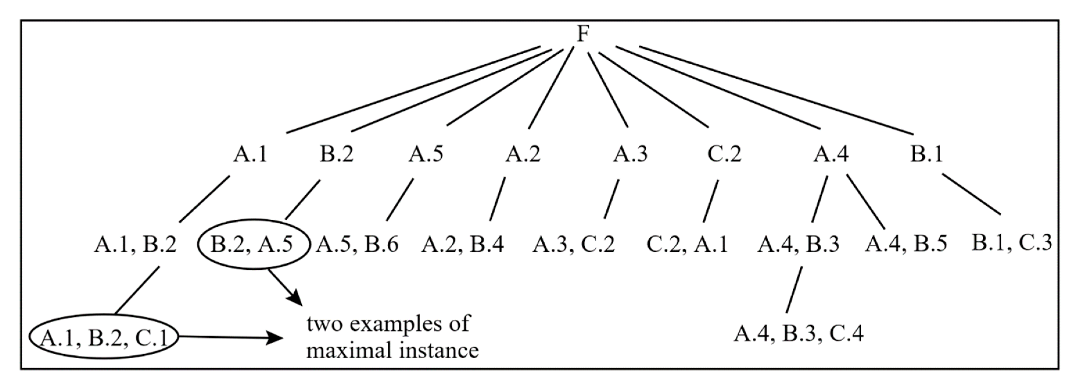
• Before building an RI-tree, all spatial instances are put into the set F. The instance will be deleted from F if a child node of the root is created for it or if it has a neighbor relationship with the child node of the root. For example, a child node of the root is created for $A.5$, so $A.5$ will be deleted from F; $B.2$ and $C.1$ are deleted from F since they have neighbor relationships with $A.5$ ($A.5$ is a child node of the root).
• Each node is a row instance of the co-location, and note that not all row instances are listed in the RI-tree but all neighbor relationships are contained in the RI-tree. The number of row instances is very large if there are a lot of instances in the spatial data. The aim of an RI-tree is to generate the maximal instance; there is no need to list all row instances in an RI-tree. A node in an RI-tree contains neighbor relationships between all instances in the node.
• The nodes of the n-th layer of an RI-tree are n-1-size row instances. The spatial instances in F are selected as the child node of the root, i.e., nodes in the second layer of the RI-tree. From layer 3 to layer n, there are size 2 row instances, size 3 row instances, $\cdots$, and n-1-size row instances. The highest size of the row instance of the example data in Figure 1 is 3 since the RI-tree constructed for this example data has only four layers.
• After creating a child node of the root, scan its neighbor relationships. The neighbor relationships are identified by the Euclidean distance metric. Two instances have a neighbor relationship if their Euclidean distance is less than the user-defined minimum distance threshold [1]. If this node has a neighbor relationship with another instance, a child node of this node will be created under this branch for these two instances; if there is no common neighbor of instances in this node, another instance will be popped from F and a child node of the root will be created for it. For example, instance $B.2$ is a child node of the root and the node “$B.2, A.5$” is created under this branch since $B.2$ has a neighbor relationship with $A.5$. There is no common neighbor of $B.2$ and $A.5$, but $A.5$ still has relationship with $B.6$, so a new child node of the root is created for $A.5$, and the node $A.5$ has “$A.5, B.6$” as a child node.
• The RI-tree is built from left to right. When a leaf node appears in one branch of the RI-tree, another branch can be established. A node is a leaf node if there is no common neighbor of instances in this node, which means the end of the branch where this node is located.
• The leaf nodes of an RI-tree are maximal instances because a leaf node is a row instance in which all instances are neighbors and no other instance can join with it to generate a high-size row instance. It is obvious that the leaf node meets the conditions of maximal instance. The number of maximal instances equals the number of branches of the RI-tree.

2.2.2. Completeness of the RI-Tree

None of the neighbor relationships is omitted in the process of finding maximal instances. All the spatial instances are scanned, and all neighbor relationships between instances of different spatial types are considered in the process of constructing an RI-tree. Although not all neighbor relationships are shown in the RI-tree, they are considered when creating nodes. For example, the node “$A.1, B.2, C.1$” contains the neighbor relationships between $A.1$ and $B.2$, $A.1$ and $C.1$, and $B.2$ and $C.1$, although the neighbor relationships between $A.1$ and $C.1$ on one hand and $B.2$ and $C.1$ on the other are not shown in the RI-tree. The neighbor relationships are also not duplicated. Once all neighbor relationships of an instance are identified, this instance will be deleted in F.

2.3. Generation of Co-Locations

Candidate co-location generation: The basic algorithms rely on a combinatorial approach and use apriori_gen [25] to generate size k+1 candidate co-locations from size-k-prevalent co-locations. However, this paper generates candidate co-locations from maximal instances, which does not require any join operations. $C=\left\{e_1, e_2, \cdots , e_k\right\}$ is a candidate co-location if $m=\left\{i_1, i_2, \cdots , i_k\right\}$ is a maximal instance, $i_n$ is an instance of spatial event types $e_n$, and $1\le n\le k$. For example, $\left\{A.1, B.2, C.1\right\}$ is a maximal instance, so $T=\left\{A, B, C\right\}$ is a candidate co-location. Candidate co-locations are also generated from candidate co-locations that are not prevalent. Candidate co-locations generated from maximal instances are not all prevalent. Candidate co-locations that fail to be a prevalent pattern are selected, and their subsets are corresponding low-size candidate co-locations. That is because of the anti-monotonicity of the participation index. If $pi\left(C\right)<min\_prev$ (C is a candidate co-location,$\mathrm{and} pi\left(C\right) \mathrm{is} \mathrm{the} \mathrm{participation} \mathrm{index} \mathrm{of} C$), there must exist $pi\left(c\right)\ge pi\left(C\right)$ (c is a subset of C) and c may be a prevalent co-location, so c is a candidate co-location. Taking Figure 1 as an example, if $min\_prev$ is set to 0.4, $T=\left\{A, B, C\right\}$ is not a prevalent co-location since $pi\left(T\right)=min\left\{pr\left(T, A\right), pr\left(T, B\right), pr\left(T, C\right)\right\}=\min (2/5,2/6,2/4)=1/3<0.4$, where pr is the participation ratio. Therefore, $\left\{A,B\right\},\left\{A,C\right\}$, and $\left\{B,C\right\}$ (subsets of $\left\{A,B,C\right\}$) are candidate co-locations.

Pruning: To make our algorithm more efficient, this step introduces the pruning strategies that can greatly reduce the unnecessary calculation time. Prevalence-based pruning [1] is also used in our algorithm. The refinement filtering of co-locations is done by the participation index values calculated from their co-location instances. Prevalent co-locations satisfying a given threshold are selected. Actually, there is no need to calculate the participation index of each candidate co-location. Because the participation ratio and the participation index are antimonotone (monotonically nonincreasing) as the size of the co-location increases [1]), if a high-size candidate co-location is prevalent, subsets of this candidate co-location are all prevalent. Therefore, participation indexes of high-size candidate co-locations (generated by maximal instances) are prioritized. If the participation index values are above a given threshold, there is no need to calculate the participation indexes of subsets of a high-size candidate co-location; if the participation index values are below a given threshold, the participation indexes of the subsets of high-size candidate co-locations need to be calculated.

The second pruning strategy can be explained by Lemma 4.

Lemma 4.

Subsets of a candidate co-location are prevalent if it is a prevalent co-location.

Proof of Lemma 4.

This lemma is proved by the antimonotone property of the participation index. $C$ is a candidate co-location; $C^{\prime }$ is a subset of $C$; and k and n ($k>n$) are the number of instances in $C$ and the number of instances in $C^{\prime }$, respectively. From the above formula, it can be concluded that the participation index of a candidate co-location is less than or equal to that of its subset. If $pi\left(C\right)<min\_prev$, then $pi\left(C^{\prime }\right)<min\_prev$ must be established, so the following conclusion can be drawn: subsets of a candidate co-location are prevalent if it is a prevalent co-location.

$$pi\left(C\right)=min\{\frac{\left|{\pi }_{e_1}\left(table\_instance\left(C\right)\right)\right|}{\left|e_1\right|}, \cdots ,$$

$$\frac{\left|{\pi }_{e_k}\left(table\_instance\left(C\right)\right)\right|}{\left|e_k\right|}\}$$

$$=mi{n}_{i=1}^k\left\{pr\left(C,e_i\right)\right\}$$

$$\le mi{n}_{i=1}^n\left\{pr\left(C,e_i\right)\right\}$$

$$\le mi{n}_{i=1}^n\left\{pr\left(C^{\prime },e_i\right)\right\}=pi\left(C^{\prime }\right).$$

 □

Quite a lot of maximal instances are generated in the process of mining co-locations from the real data set introduced in Section 4. $\left\{A, I, T, P, R\right\}$ is a candidate co-location since there are row instances of $\left\{A, I, T, P, R\right\}$ in maximal instances, and $\left\{A, I, T, P, R\right\}$ is the highest-size candidate co-location since there are only five facility types in the real data set. The participation index of $\left\{A, I, T, P, R\right\}$ is calculated first. When $min\_d$ is set to 1, $pi\left(\left\{A, I, T, P, R\right\}\right)=0.1$. $\left\{A, I, T, P, R\right\}$ fails to be a prevalent co-location if $min\_prev$ is set to 0.4. Therefore, $\left\{A, I, T, P\right\}$, $\left\{A, I, T, R\right\}$, $\left\{A, I, P, R\right\}$, $\left\{A, T, P, R\right\}$, and $\left\{I, T, P, R\right\}$, which are the subsets of $\left\{A, I, T, P, R\right\}$, become candidate co-locations. In the subsets of $\left\{A, I, T, P, R\right\}$, those row instances that contain four instances are row instances of size 4 co-locations. The size 4 maximal instances are also row instances of size 4 co-locations. By calculating their participation indexes, it is clear that $\left\{A, T, P, R\right\}$ is a prevalent co-location with $pi\left(\left\{A, T, P, R\right\}\right)=0.48$. According to the anti-monotonicity of the participation index, the participation indexes of $\left\{A, T, P\right\}$, $\left\{A, T, R\right\}$, $\left\{A, P, R\right\}$, and $\left\{T, P, R\right\}$ must be greater than 0.48. $\left\{A, T, P\right\}$, $\left\{A, T, R\right\}$, $\left\{A, P, R\right\}$, and $\left\{T, P, R\right\}$ are prevalent co-locations, so there is no need to calculate their participation indexes, which saves a lot of time. This is the pruning strategy mentioned above.

2.4. Discussions for Maximal Instance Algorithm

The idea of the presented algorithm is different from the existing algorithms. The differences are as follows:

• The existing methods identify high-size row instances from low-size row instances, but the presented algorithm first identifies the highest-size row instances (maximal instances) based on the relationship of spatial instances and then generates all low-size row instances from highest-size row instances.
• The existing methods generate candidate patterns by joining row instances, but the presented algorithm generates candidate patterns from maximal instances without join operations.

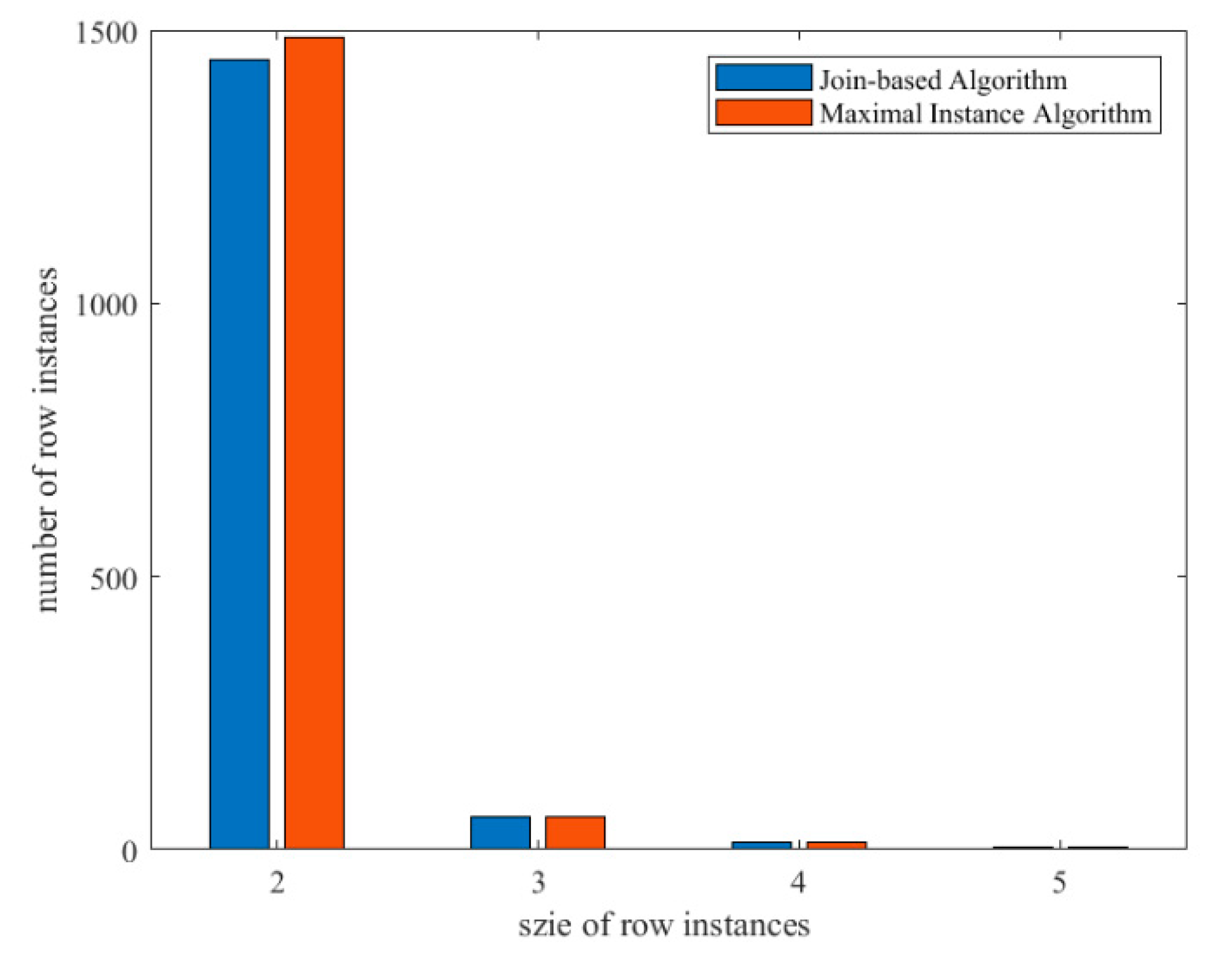
2.4.1. Comparison Analysis of Row Instance Generation

The reason why our method for generating all row instances is more efficient than the join-based algorithm is demonstrated in detail here. Let $T_{gen\_row instance}$ and $T_{gen\_row instance}^{’}$ be the computation cost of generating all row instances by the join-based algorithm and our method. The following equations show the computation cost functions:

$$T_{gen\_row instance}=T_{scan\left(neighobr relationship\right)}+\left(k-1\right)\times T_{join}$$

(3)

$$T_{gen\_row instance}^{’}=T_{gen\_m}+T_{gen\_instance}$$

(4)

$T_{join}$ represents the computation cost of a join operation, $T_{gen\_m}$ represents the computation cost of generating all maximal instances, and $T_{gen\_instance}$ represents the computation cost of finding the subsets of maximal instances. $T_{gen\_m}\approx T_{scan\left(neighobr relationship\right)}$ because generating maximal instances is also a scanning process of neighbor relationship and $T_{gen\_instance}\ll \left(k-1\right)\times T_{join}$.

Therefore,

$$\begin{array}{c}\frac{T_{gen\_row instance}}{T_{gen\_row instance}^{’}}=\frac{T_{scan\left(neighobr relationship\right)}+\left(k-1\right)\times T_{join}}{T_{gen\_m}+T_{gen\_instance}}\\ \approx \frac{T_{scan\left(neighobr relationship\right)}+\left(k-1\right)\times T_{join}}{T_{scan\left(neighobr relationship\right)}+T_{gen\_instance}}\\ >1.\end{array}$$

Apparently, $T_{gen\_row instance}>T_{gen\_row instance}^{’}$. So the conclusion can be drawn that our method of generating all row instances is more efficient than the join-based algorithm.

2.4.2. Comparison Analysis of Maximal Instance Algorithm

The computational cost of our algorithm with three basic algorithms is compared here. Each algorithm has an initial step of materializing neighborhoods. The join-based algorithm first gathers the neighbor pairs per candidate co-location, the partial-join algorithm first generates the disjoint clique neighborhoods using a simple grid partitioning, the join-less algorithm first generates the star neighborhoods, and our algorithm first generates maximal instances. S represents a spatial data set; $T_{neighbor\_pairs}\left(S\right)$, $T_{clique\_neighborhoods\&cut\_relations}\left(S\right)$, $T_{star\_neighborhoods}\left(S\right)$, and $T_{gen\_m}\left(S\right)$ represent the computational costs of the initial steps in each algorithm; and $T_{jb}\left(2\right)$, $T_{pj}\left(2\right)$, and $T_{jl}\left(2\right)$ represent the cost of generating size 2 co-locations in the join-less algorithm, the partial-join algorithm, and the join-based algorithm, respectively. Let $T, T_{jl}, T_{pj}$, and $T_{jb}$ be the total computation cost of our algorithm, the join-less algorithm, the partial-join algorithm, and the join-based algorithm, respectively. The following equations show the total cost functions:

$$T=T_{gen\_m}\left(S\right)+T_{gen\_instance},$$

$$T_{jl}=T_{star\_neighborhoods}\left(S\right)+T_{jl}\left(2\right)+{{\displaystyle \sum }}_{k>2}{T}_{jl}\left(k\right),$$

$$T_{pj}=T_{clique\_neighborhoods\&cut\_relations}\left(S\right)+T_{pj}\left(2\right)+{{\displaystyle \sum }}_{k>2}{T}_{pj}\left(k\right),$$

$$T_{jb}=T_{neighbor\_pairs}\left(S\right)+T_{jb}\left(2\right)+{{\displaystyle \sum }}_{k>2}{T}_{jb}\left(k\right),$$

Here, k is greater than 2.

Yoo and Shekhar [5] proposed the following comparative relationships:

$$T_{clique\_neighborhoods\&cut\_relations}\left(S\right)+T_{pj}\left(2\right)$$

$$>T_{star\_neighborhoods}\left(S\right)+T_{jl}\left(2\right),$$

$$>T_{neighbor\_pairs}\left(S\right)+T_{jb}\left(2\right)$$

because (1) the join-less algorithm involves an additional cost to generate the star neighborhoods from the neighbor pairs compared with join-based algorithm and (2) an additional cost is incurred when finding all size 2 inter-instances with cut relationships in the partial-join algorithm, the overall cost is expected to be a little greater than the cost to generate the star neighborhood set.

Lemma 5.

$T_{star\_neighborhoods}\left(S\right)>T_{gen\_m}\left(S\right)$.

Proof of Lemma 5.

The star neighborhood partition model in the join-less algorithm takes each spatial object as a central object and finds out the remaining objects in its neighborhood. Thus, this process is performed n times, where n is the number of spatial objects. The process of generating all maximal instances needs to be executed $\left|C_m\right|$ times, where $\left|C_m\right|$ is the number of maximal instances. Apparently, $n>\left|C_m\right|$, so the star neighborhood partition model in the join-less method is more time consuming than the process of generating the maximal instance in our method.

$$\frac{T_{star\_neighborhoods}\left(S\right)}{T_{gen\_m}\left(S\right)}\approx \frac{n\times t_{scan\left(neighbor relationship\right)}}{\left|C_m\right|\times t_{scan\left(neighbor relationship\right)}}$$

$$=\frac{n}{\left|C_m\right|}$$

$$>1.$$

 □

Lemma 6.

$T_{gen\_m}\left(S\right)>T_{neighbor\_pairs}\left(S\right)+T_{jb}\left(2\right)$.

Proof of Lemma 6.

Gathering the neighbor pairs per candidate co-location is the most basic operation in co-location mining. The neighbor pairs are used to generate maximal instances, and it involves additional cost compared with gathering the neighbor pairs per candidate co-location and calculating their prevalence measures. □

According to Lemma 5 and Lemma 6, the following equation can be reached:

$$\begin{array}{c}{T}_{clique\_neighborhoods\&cut\_relations}\left(S\right)+T_{pj}\left(2\right)\\ >T_{star\_neighborhoods}\left(S\right)+T_{jl}\left(2\right)\\ >T_{gen\_m}\left(S\right)\\ >T_{neighbor\_pairs}\left(S\right)+T_{jb}\left(2\right).\end{array}$$

(5)

The advantage of the maximal instance algorithm lies in the latter part. Three basic algorithms generate bigger-size co-locations size by size after generating size 2 co-locations. This operation needs to be repeated k-2 times to generate all co-locations. No operation can be omitted, and a cross-size operation is not allowed (size k co-locations cannot be directly generated from size k-2 co-locations; size k co-locations are generated from size k-1 co-locations after generating size k-1 co-locations from size k-2 co-locations). Therefore, the execution time of each join operation should be added to the total computational costs of the three basic algorithms.

However, once the maximal instance algorithm generates maximal instances, row instances of all size co-locations can be generated from the subsets of maximal instances. There is no need for a join operation. A large amount of time consumption is avoided in this part; the bigger the size of the co-locations, the more obvious the effect, and thus the following equations:

$$T_{gen\_instance}\ll {{\displaystyle \sum }}_{k>2}{T}_{jl}\left(k\right),$$

(6)

$$T_{gen\_instance}\ll {{\displaystyle \sum }}_{k>2}{T}_{pj}\left(k\right),$$

(7)

$$T_{gen\_instance}\ll {{\displaystyle \sum }}_{k>2}{T}_{jb}\left(k\right).$$

(8)

On the basis of Equations (5)–(8), we can say that our algorithm has a lower computational cost than the three basic algorithms.

$$T<T_{jl},$$

$$T<T_{pj},$$

$$T<T_{jb}.$$

2.5. Overview of the Maximal Instance Algorithm

This section introduces the steps in the maximal instance algorithm. As shown in Figure 4, this algorithm has four steps in the flow chart. The participation index is still used as the prevalence measure to determine whether a co-location pattern is prevalent. As shown in Figure 5, the maximal instance algorithm takes a set E of spatial event types, a set I of instances, a distance threshold $min\_d$, and a minimal prevalent threshold $min\_prev$. The algorithm outputs a correct set of co-location patterns with participation index $>min\_prev$. The set $C_1$ of candidate size 1 co-locations and the set $P_1$ of prevalent size 1 co-locations are initialized to E, since the value of the participate index is 1 for all size 1 co-locations. The set $R{I}_1$ of row instances of size 1 co-locations is initialized to I.

Step 1 (maximal instance generation): Our algorithm aims to find the maximal instances first, which is the key to co-location mining. A set of spatial instances with their spatial relationships (i.e., Euclidean distance) is input, each instance is a vector $\mathrm{instance}-\mathrm{id}, \mathrm{location}, \mathrm{spatial} \mathrm{feature} \mathrm{type}$, and an algorithm implemented in Python outputs all maximal instances. In this process, the neighbor relationships between instances of the same spatial feature type are not taken into consideration since our goal is to find the positive relationship between different spatial feature types.

Step 2 (row instance generation): Row instances of co-locations are generated by finding subsets of maximal instances instead of join operations between row instances.

Step 3 (candidate co-location generation): $C=\left\{e_1, e_2, \cdots , e_k\right\}$ is a candidate co-location if $m=\left\{i_1, i_2, \cdots , i_k\right\}$ is a maximal instance, $i_n$ is an instance of spatial event types $e_n$, and $1\le n\le k$. For example, $\left\{A.1, B.2, C.1\right\}$ is a maximal instance, so $T=\left\{A, B, C\right\}$ is a candidate co-location, and a candidate co-location is also generated from candidate co-locations that are not prevalent.

Step 4 (pruning): There are two pruning strategies in the maximal instance algorithm: (1) prevalence-based pruning is also used in our algorithm, and (2) participation indexes of high-size candidate co-locations (generated by maximal instances) are prioritized. If the participation index values are above a given threshold, there is no need to calculate the participation indexes of subsets of the high-size candidate co-location; if the participation index values are below a given threshold, the participation indexes of subsets of high-size candidate co-locations need to be calculated.

3. Experiments

In this section, experiments are carried with synthetic data sets and a real data set to evaluate our algorithm.

3.1. Synthetic Data Set

The synthetic data sets are generated in Python, as shown in Figure 6. There are 60 different spatial event types in a synthetic data set. The number of instances of each spatial feature stored in the set Value is a random number between 5 and 10. E is a set of all spatial event types, and I is a set of instances. Each instance is a point distributed in a spatial framework $D_1\times D_2$ (150$\times$100), and these point data have their own unique coordinates. The neighbor relationships of the synthetic data sets are generated by calculating the Euclidean distance of those points and stored in the set R.

3.2. Real Data Set

The real data set is about college and university locations, hospital locations, library locations, nursing home locations from Maine E911 address data from MainePUC, and point locations of the mineral collecting sites in Maine [26]. Each event in this data set with a different spatial feature types has a unique event ID. Contained in each event is county, town, latitude, longitude, and other information. Location information with only latitude and longitude is considered in this experiment. The event numbers of spatial feature types are shown in

Table 2. Description of event numbers of spatial feature types.

Spatial Feature Type	Abbreviation	Number of Events
College and University	U	286
Hospital	H	74
Library	L	83
Nursing Home	N	45
Mineral Collecting Site	M	32

.

3.3. Experiment Results

A summary of our experiment result is presented here. A real data set of college and university locations, hospital locations, library locations, nursing home locations from Maine E911 address data from MainePUC, and point locations of the mineral collecting sites in Maine is studied in this paper. The longitude and latitude of each facility are used as coordinates to calculate the Euclidean distance. The effects of $min\_d$ on the number of neighbor relationships, participation ratio, and participation index are evaluated. Table 2 shows the number of events for each spatial feature type in the real data set.

Table 3. The participation indexes of co-location patterns.

Co-Location Patterns	$\mathbf{Participation} \mathbf{Indexes} (\mathit{m}\mathit{i}\mathit{n}\_\mathit{d} \mathbf{Is} \mathbf{Set} \mathbf{to} 0.4)$
$\left\{U,H\right\}$	0.61
$\left\{U, L\right\}$	0.63
$\left\{H,L\right\}$	0.81
$\left\{U, H, L\right\}$	0.59
$\left\{U, H, N\right\}$	0.53
$\left\{U, H, M\right\}$	0.44
$\left\{U, L, N\right\}$	0.73
$\left\{U, L, M\right\}$	0.47
$\left\{U, N, M\right\}$	0.41

shows the participation indexes of co-location patterns. When $min\_d$ is set to 0.4 and $min\_prev$ is set to 0.5, co-location patterns $\left\{U, H\right\}$, $\left\{U, L\right\}$, $\left\{H, L\right\}$, $\left\{U, H, L\right\}$, $\left\{U, H, N\right\}$, and $\left\{U, L, N\right\}$ are prevalent and their participation indexes are 0.61, 0.63, 0.81, 0.59, 0.53, and 0.73, respectively. The co-location $\left\{U, H\right\}$ means hospitals are frequently located together in a geographic space with colleges and universities. For example, the University of Southern Maine is adjacent to two hospitals in the south, namely Maine Medical Center and Northern Light Mercy Hospital. The co-location $\left\{U, L\right\}$ means libraries are frequently located together in a geographic space with colleges and universities. This is mainly because some libraries are located inside universities and colleges. For example, the largest library in Maine, the Fogler Library, is located in the University of Maine.

The result quality comparison

Firstly, the quality of the generated maximal instance is tested in terms of the total number of maximal instances, the number of maximal instances per size, and the number of maximal instances with errors and repetitions. The quality result of the maximal instances is shown in the

Table 4. The quality of maximum instances.

	Number
Maximal Instances	1342
Size 2 Maximal Instances	1268
Size 3 Maximal Instances	17
Size 4 Maximal Instances	5
Size 5 Maximal Instances	3
False	7
Repetitive	42

. There are 1342 maximal instances in total. After removing the repetition, the number of size 2, size 3, size 4, and size 5 maximal instances is 1268, 17, 5, and 3, respectively. These 1342 maximal instances are not all correct. Among them, seven maximal instances with a size greater than 5 are errors. The maximum size of maximal instances is 5 since there are only five feature types in the real data set. Moreover, there are 42 repeated maximal instances in the size 2 maximal instances, but this phenomenon does not appear in the other higher-size maximal instances. It can be seen that the quality of the generated maximal instances is relatively good. These maximal instances of errors and repetitions have little effect on the experimental results.

Figure 7 shows a comparison of row instances generated by the join-based algorithm a and the maximal instance algorithm. Row instance is the basis of co-location participation index. Only when the number of row instances is clear can the participation index of co-locations be calculated and whether co-locations are frequent be judged. Therefore, this paper used the join-based algorithm and the maximal instance algorithm to generate all the row instances, recorded the number of row instances in each size, and made a comparison. The results show that the number of size 3, size 4, and size 5 row instances generated by the two algorithms is the same and only the number of size 2 row instances is slightly different. The maximal instance algorithm generates 42 more size 2 row instances than the join-based algorithm, which is because the maximal instance algorithm generates 42 repeated maximal instances in the size 2 maximal instances. The impact of these 42 row instances on participation is very small.

On comparing the results, it is clear that the maximal instance algorithm only has a slight difference in the size 2 instance, which will not have a great impact on the quality of the generated co-locations.

Effect of$\mathit{min}\_\mathit{d}$on the number of neighbor relationships

The effects of $min\_d$ on the number of neighbor relationships are evaluated. The value of $min\_d$ is changed while the other experimental parameters remain unchanged. The number of neighbor relationships between any two spatial feature types is checked successively. The result is shown in Figure 8. In general, the number of neighbor relationships between any two types increases with an increase in the value of $min\_d$. With the increase in $min\_d$, the numbers of neighbor relationships of $\left\{U, H\right\}$ and $\left\{U, L\right\}$ are far more than that of other patterns. Because of the large number of events of type U, H, and L, the numbers of neighbor relationships of $\left\{U, H\right\}$ and $\left\{U, L\right\}$ increase sharply to more than 7000 when $min\_d$ increases to 0.9.

Effect of$\mathit{min}\_\mathit{d}$on participation ratio and participation index

The effects of $min\_d$ on participation ratio and participation index are evaluated. The value of the parameter $min\_d$ is changed to observe the values of the participation ratio and the participation index of co-locations. Figure 9 shows the change in the participation ratio of co-locations $\left\{U, H, L\right\}$, $\left\{U, H, N\right\}$, $\left\{U, H, M\right\}$, $\left\{U, L, M\right\}$, $\left\{U, L, N\right\}$, and $\left\{U, N, M\right\}$. It is obvious that the values of the participation ratio increase with an increase in $min\_d$. The changes in the participation indexes of different co-locations are shown in Figure 10a,b. The following observations can be made:

(1)

$pi\left(\left\{U, H, L\right\}\right)$ (the value of the participation index of $\left\{U, H, L\right\}$) is always smaller than $pi\left(\left\{U, H\right\}\right)$, $pi\left(\left\{U, L\right\}\right)$, and $pi\left(\left\{H, L\right\}\right)$, and the same is the case in Figure 10b, where $pi\left(\left\{U, H,N\right\}\right)$ is always smaller than $pi\left(\left\{U, H\right\}\right)$, $pi\left(\left\{U, N\right\}\right)$, and $pi\left(\left\{H,N\right\}\right)$. This is because the participation ratio and the participation index are antimonotone (monotonically nonincreasing) as the size of the co-location increases [1] and it shows that our results are correct.

(2)

The combination of the minimum values of the three curves in Figure 9a is the curve of $pi\left(\left\{U, H,L\right\}\right)$ in Figure 10a, since the $pi\left(C\right)$ of a co-location $C=\left\{e_1,\cdots ,e_k\right\}$ is defined as $mi{n}_{i=1}^k\left\{pr\left(C,e_i\right)\right\}$.

3.4. Experimental Evaluation

The synthetic data sets are used to check whether our algorithm has better performance. Two comparative experiments on running time were done to evaluate the performance of the maximal instance algorithm. As shown in Figure 11, the running time of generating row instances is compared when $min\_d$ changes. The time to generate maximal instances is used to indicate the time to generate row instances of the maximal instance algorithm, because once maximal instances are found, row instances are found. The result shows that the running time increases with an increase in $min\_d$ and the maximal instance algorithm consumes less time. Figure 12 shows the effect of the number of spatial instances on the running time, and no matter how the number of spatial instances changes, the maximal instance algorithm still consumes less time. Obviously, the maximal instance algorithm has better performance in the process of generating prevalent co-locations since there is no need for join operations in the maximal instance algorithm. Therefore, it can be concluded that the maximal instance algorithm is more efficient than the three basic algorithms.

4. Conclusions and Future Work

This paper proposes a new concept of maximal instances that is fundamental to our work and proves that generating row instances by maximal instances can make sense. A comparison with generating row instances by join operations proves that generating row instances by maximal instances is more efficient. An RI-tree is constructed to find maximal instances from a spatial data set. The proposed algorithm, the maximal instance algorithm, is based on maximal instances to mine co-location patterns. Since join operations are needed in this algorithm, it can reduce a lot of computing time. A detailed comparison with the three basic algorithms (join-based algorithm, partial-join algorithm, join-less algorithm) shows the advantage of our algorithm in terms of time consumption.

Synthetic data sets and a real data set are used to examine the effect of our algorithm. The real data set is about college and university locations, hospital locations, library locations, nursing home locations from Maine E911 address data from MainePUC, and point locations of the mineral collecting sites in Maine. This data set has five spatial feature types: college and university, hospital, library, nursing home, and mineral collecting site. The prevalent co-locations $\left\{U, H\right\}$, $\left\{U, L\right\}$, $\left\{H, L\right\}$, $\left\{U, H, L\right\}$, $\left\{U, H, N\right\}$, and $\left\{U, L, N\right\}$ are generated when $min\_d$ is set to 0.4 and $min\_prev$ is set to 0.5 ($pi\left(\left\{U, H\right\}\right)=0.61, pi\left(\left\{U, L\right\}\right)=0.63, pi\left(\left\{H, L\right\}\right)=0.81, pi\left(\left\{U, H, L\right\}\right)=0.59,$ $pi\left(\left\{U, H, N\right\}\right)=0.53$, $pi\left(\left\{U,L, N\right\}\right)=0.73$). The participation indexes of the co-locations vary with a change in the experimental parameter $min\_d$ and satisfy anti-monotonicity, and comparative experiments on running time show that the maximal instance algorithm has better performance.

Many application domains include spatio-temporal features. Scientists in these domains are interested in understanding the evolution of the co-location patterns among stationary features as well as co-location patterns over moving feature types. In future work, it will be interesting to explore methods to answer temporal questions such as how a co-location changes over time as well as methods to identify moving object co-location patterns.

References

1. Huang, Y.; Shekhar, S.; Xiong, H. Discovering colocation patterns from spatial data sets: A general approach. IEEE Trans. Knowl. Data Eng. 2004, 16, 1472–1485. [Google Scholar] [CrossRef] [Green Version]
2. Shekhar, S.; Huang, Y. Discovering Spatial co-location patterns: A summary of results. In Advances in Spatial and Temporal Databases; Jensen, C.S., Schneider, M., Seeger, B., Tsotras, V.J., Eds.; Springer: Berlin/Heidelberg, Germany, 2001; p. 2121. [Google Scholar]
3. Yoo, J.S.; Shekhar, S.; Smith, J.; Kumquat, J.P. A partial join approach for mining co-location patterns. In Proceedings of the 12th annual ACM international workshop on Geographic information systems—GIS ’04, Washington, DC, USA, 12–13 November 2004; pp. 241–249. [Google Scholar] [CrossRef]
4. Yoo, J.S.; Shekhar, S.; Celik, M. A Join-Less Approach for Co-Location Pattern Mining: A Summary of Results. In Proceedings of the Fifth IEEE International Conference on Data Mining (ICDM’05), Houston, TX, USA, 27–30 November 2005; p. 4. [Google Scholar]
5. Yoo, J.S.; Shekhar, S. A join-less approach for mining spatial co-location pattern. IEEE Trans. Knowl. Data Eng. 2006, 18, 1323–1337. [Google Scholar]
6. Djenouri, Y.; Lin, J.C.-W.; Nørvåg, K.; Ramampiaro, H. Highly Efficient Pattern Mining Based on Transaction Decomposition. In Proceedings of the 2019 IEEE 35th International Conference on Data Engineering (ICDE), Macao, China, 8–11 April 2019; pp. 1646–1649. [Google Scholar]
7. Zhang, B.; Lin, J.C.-W.; Shao, Y.; Fournier-Viger, P.; Djenouri, Y. Maintenance of Discovered High Average-Utility Itemsets in Dynamic Databases. Appl. Sci. 2018, 8, 769. [Google Scholar] [CrossRef] [Green Version]
8. Huang, Y.; Pei, J.; Xiong, H. Mining Co-Location Patterns with Rare Events from Spatial Data Sets. GeoInformatica 2006, 10, 239–260. [Google Scholar] [CrossRef] [Green Version]
9. Verhein, F.; Al-Naymat, G. Fast Mining of Complex Spatial Co-location Patterns Using GLIMIT. In Proceedings of the Seventh IEEE International Conference on Data Mining Workshops (ICDMW 2007), Omaha, NE, USA, 28–31 October 2007; pp. 679–684. [Google Scholar]
10. Al-Naymat, G. Enumeration of maximal clique for mining spatial co-location patterns. In Proceedings of the 2008 IEEE/ACS International Conference on Computer Systems and Applications, Doha, Qatar, 31 March–4 April 2008; pp. 126–133. [Google Scholar]
11. Kim, S.K.; Kim, Y.; Kim, U. Maximal cliques generating algorithm for spatial colocation pattern mining. In Secure and Trust Computing, Data Management and Applications; Park, J.J., Lopez, J., Yeo, S.S., Shon, T., Taniar, D., Eds.; Springer: Berlin/Heidelberg, Germany, 2011; Volume 186, pp. 241–250. [Google Scholar]
12. Yao, X.; Wang, D.; Peng, L.; Chi, T. An adaptive maximal co-location mining algorithm. In Proceedings of the 2017 IEEE International Geoscience and Remote Sensing Symposium (IGARSS), Fort Worth, TX, USA, 23–28 July 2017; pp. 5551–5554. [Google Scholar] [CrossRef]
13. Deng, M.; Cai, J.; Liu, Q.; He, Z.; Tang, J. Multi-level method for discovery of regional co-location patterns. Int. J. Geogr. Inf. Sci. 2017, 31, 1–25. [Google Scholar] [CrossRef]
14. Huang, Y.; Zhang, P.; Zhang, C. On the Relationships between Clustering and Spatial Co-Location Pattern Mining. Int. J. Artif. Intell. Tools 2008, 17, 55–70. [Google Scholar] [CrossRef] [Green Version]
15. Jiamthapthaksin, R.; Eick, C.F.; Vilalta, R. A framework for multi-objective clustering and its application to co-location mining. In Advanced Data Mining and Applications; Huang, R., Yang, Q., Pei, J., Gama, J., Meng, X., Li, X., Eds.; Springer: Berlin/Heidelberg, Germany, 2009; Volume 5678, pp. 188–199. [Google Scholar]
16. Yu, W. Identifying and Analyzing the Prevalent Regions of a Co-Location Pattern Using Polygons Clustering Approach. ISPRS Int. J. Geo-Infor. 2017, 6, 259. [Google Scholar] [CrossRef] [Green Version]
17. Ouyang, Z.; Wang, L.; Wu, P. Spatial Co-Location Pattern Discovery from Fuzzy Objects. Int. J. Artif. Intell. Tools 2017, 26. [Google Scholar] [CrossRef] [Green Version]
18. Zhou, G.; Wang, L. Co-location decision tree for enhancing decision-making of pavement maintenance and rehabilitation. Transp. Res. Part C: Emerg. Technol. 2012, 21, 287–305. [Google Scholar] [CrossRef] [Green Version]
19. Zhou, G.; Zhang, R.; Zhang, D. Manifold Learning Co-Location Decision Tree for Remotely Sensed Imagery Classification. Remote Sens. 2016, 8, 855. [Google Scholar] [CrossRef] [Green Version]
20. Zhou, G.; Li, Q.; Deng, G.; Yue, T.; Zhou, X. Mining Co-Location Patterns with Clustering Items from Spatial Data Sets. ISPRS-Int. Arch. Photogramm. Remote Sens. Spat. Inf. Sci. 2018, XLII-3, 2505–2509. [Google Scholar] [CrossRef] [Green Version]
21. Bao, X.; Wang, L. A clique-based approach for co-location pattern mining. Inf. Sci. 2019, 490, 244–264. [Google Scholar] [CrossRef]
22. Celik, M.; Kang, J.M.; Shekhar, S. Zonal co-location pattern discovery with dynamic parameters. In Proceedings of the Seventh IEEE International Conference on Data Mining, Omaha, NE, USA, 28–31 October 2007. [Google Scholar]
23. Jiang, Y.; Wang, L.; Chen, H. Discovering both positive and negative co-location rules from spatial data sets. Software Engi-neering and Data Mining (SEDM). In Proceedings of the 2010 2nd International Conference on IEEE, Chengdu, China, 23–25 June 2010. [Google Scholar]
24. Yu, P. FP-Tree. based Spatial Co-Location Pattern Mining; University of North Texas: Denton, TX, USA, 2005. [Google Scholar]
25. Agrawal, R.; Srikant, R. Fast algorithms for mining association rules. In Readings in Database Systems, 3rd ed.; Stonebraker, M., Hellerstein, J.M., Eds.; Morgan Kaufmann Publishers Inc.: San Francisco, CA, USA, 1998; pp. 580–592. [Google Scholar]
26. ArcGIS Hub. Available online: https://hub.arcgis.com/ (accessed on 20 February 2021).
Figure 1. (a) An example data set; (b) instance joins.
Remotesensing 13 00960 g001
Figure 2. Algorithm for generating maximal instances.
Remotesensing 13 00960 g002
Figure 3. The process of constructing a row instance (RI)-tree.
Remotesensing 13 00960 g003
Figure 4. The flow of the maximal instance algorithm.
Remotesensing 13 00960 g004
Figure 5. Algorithm for generating co-location patterns.
Remotesensing 13 00960 g005
Figure 6. Generation process of a synthetic data set.
Remotesensing 13 00960 g006
Figure 7. Comparison of row instances generated by the join-based algorithm a and the maximal instance algorithm.
Remotesensing 13 00960 g007
Figure 8. (a) The number of neighbor relationships of { U ,   L } , { U ,   M } , { U ,   N } , { U ,   H } and { H ,   L } ; (b) the number of neighbor relationships of { H ,   N } , { H ,   M } , { L , M } , { L ,   N } and { M ,   N } .
Remotesensing 13 00960 g008
Figure 9. (a) Pr of co-location { U ,   H ,   L } ; (b) Pr of co-location { U ,   H ,   N } ; (c) Pr of co-location { U ,   H ,   M } ; (d) Pr of co-location { U ,   L ,   M } ; (e) Pr of co-location { U ,   L , N } ; (f) Pr of co-location { U ,   N ,   M } .
Remotesensing 13 00960 g009
Figure 10. (a) Pi of { U ,   H ,   L } , { U ,   H } , { U ,   L } and { H ,   L } ; (b) Pi of { U ,   H ,   N } , { U ,   H } , { U ,   N } and { H ,   N } .
Remotesensing 13 00960 g010
Figure 11. The effect of m i n _ d on the running time.
Remotesensing 13 00960 g011
Figure 12. The effect of the number of spatial instances on the running time.
Remotesensing 13 00960 g012