Article

Semi-Supervised Learning for Seismic Impedance Inversion Using Generative Adversarial Networks

School of Mathematics and Statistics, Xi’an Jiaotong University, Xi’an 710049, China
*
Author to whom correspondence should be addressed.
Remote Sens. 2021, 13(5), 909; https://doi.org/10.3390/rs13050909
Submission received: 31 December 2020 / Revised: 14 February 2021 / Accepted: 22 February 2021 / Published: 28 February 2021

Abstract

:
Seismic impedance inversion is essential to characterize hydrocarbon reservoir and detect fluids in field of geophysics. However, it is nonlinear and ill-posed due to unknown seismic wavelet, observed data band limitation and noise, but it also requires a forward operator that characterizes physical relation between measured data and model parameters. Deep learning methods have been successfully applied to solve geophysical inversion problems recently. It can obtain results with higher resolution compared to traditional inversion methods, but its performance often not fully explored for the lack of adequate labeled data (i.e., well logs) in training process. To alleviate this problem, we propose a semi-supervised learning workflow based on generative adversarial network (GAN) for acoustic impedance inversion. The workflow contains three networks: a generator, a discriminator and a forward model. The training of the generator and discriminator are guided by well logs and constrained by unlabeled data via the forward model. The benchmark models Marmousi2, SEAM and a field data are used to demonstrate the performance of our method. Results show that impedance predicted by the presented method, due to making use of both labeled and unlabeled data, are better consistent with ground truth than that of conventional deep learning methods.

1. Introduction

Seismic data are nonlinearly related to the Earth’s model parameters. Physical properties of subsurface medium such as P and S wave velocity, density and impedance (product of density and seismic velocity) can be inferred from seismic data by solving an inverse problem. The commonly used inversion methods in field of geophysics such as impedance inversion, AVO inversion and full waveform inversion aim to obtain the Earth model for which the predicted data best fit the observed seismic data [1,2,3,4,5]. Seismic impedance inversion is an effective technique for reservoir characterization and fluid prediction. However, seismic impedance inversion is usually ill-posed, nonlinear and non-unique because of unknown seismic wavelet, observed data with band limitation and various noise. It is necessary to regularize the results by imposing some constraints on the solution space or incorporating prior knowledge (i.e., well log data) into the model space to make the inverse problem well-posed. The problem of seismic inversion can be traditionally solved by two typical approaches: deterministic and stochastic methods [2,6,7] through an optimization routine. Moreover, the classical geophysical inversion needs to know the forward operator that characterizes the physical relation between the measured data and the model parameters such as wave equations or the convolution model. However, it is hard, if not impossible, to get the accurate forward model in the real subsurface surroundings. The wave equation or convolution model is always an approximation of the wave propagation or relationship between measured seismic data and physical parameters due to complexity of the medium in geological structures and environments, saturated fluids, etc. In recent years, machine learning has been popularized and successfully applied in different fields such as computer science, information engineering and geophysics. Machine learning especially deep learning methods have shown great potential for different tasks in the field of geophysics such as seismic inversion, interpretation and seismic signal recognition [8,9,10,11,12,13,14,15,16,17,18,19,20,21,22]. Machine learning, a data driven method, is a powerful tool that utilizes the neural networks to approximate the nonlinear mapping between the data space and the model space by weighted nonlinear basis functions. It has been proven to be effective to solve nonlinear inverse problems when noise exists which is common in geophysical data. Yuji Kim et al. compared the geophysical inversion based on the least-squares method with the machine learning (artificial neural networks) approach to solve the reflectivity inversion and they concluded that machine learning, especially deep learning, displays inversion results with higher resolution than that of the geophysical inversion [23]. Recently, supervised learning algorithms have been explored for seismic inversion intensively, i.e., Motaz et al. (2018) utilized recurrent neural networks for petrophysical parameters estimation [24]. Das et al. and Wu et al. used convolutional neural networks (CNNs) to invert seismic impedance by training the network using the synthetic seismograms on the earth models constrained by rock physics relations and their results showed that the prediction of the trained network are sensitive to the depositional facies type and source wavelet parameters used in the training data set [12,25]. Mustafa et al. used Temporal Convolutional Network (TCN) to estimate acoustic impedance, which not only successfully captured the long-term trends but also preserved the local patterns [26]. Du et al. proposed SeisInv-ResNet for pre-stack seismic inversion to obtain the P-wave impedance, S-wave impedance and other rock physics parameters [27]. However, the supervised-learning algorithms are given a set of measurement and labeled data as inputs, thus, a big challenge for those methods is the lack of labeled data. On the other hand, the effectiveness of deep learning methods highly depends on the quantity and diversity of the training data set. In seismic impedance inversion, the well log data are main source of the training labels, which are limited in real case due to high cost. An alternative approach to overcome this problem is taking advantage of both labeled and unlabeled data. To this end, Alfarraj et al. proposed a semi-supervised machine learning workflow for acoustic impedance inversion from zero-offset seismic data by combining an inverse model based on CNN and recurrent neural networks (RNN) with a forward model that is based on the Aki-Richards approximation, in which they used a learned seismic forward model as a geophysical constraint to regularize the training process of inversion [28]. Wang et al. introduced cycle-consistent generative adversarial network (Cycle-GAN) for impedance inversion and the Cycle-GAN had a better performance than the conventional CNN method by making use of the unlabeled data [10]. Cai et al. employed the Wasserstein cycle-consistent GAN (WCycle-GAN) by integrating the Wasserstein loss with gradient penalty loss as the target loss function to improve the performance of Cycle-GAN [29].
In this paper, we propose a semi-supervised learning workflow for seismic impedance inversion based on GAN. A CNN is trained as a seismic forward model to learn seismic traces from impedance and then the GAN is trained which is supervised by limited well logs and constrained by the forward model. The remainder of this paper is organized as follows. In Section 2, we briefly introduce the theory of GAN and the architecture of networks including the generator, the discriminator and the forward model, as well as the formulation and training details of the proposed method. In Section 3, we present, analyze and discuss the experimental results on two types of typical seismic models such as 2-D Marmousi2, an inline section of 3-D SEAM model and a field dataset. The experimental results are further compared with that of CNN and other state-of-the-art deep learning algorithms. Finally, Section 4 summarizes this paper.

2. GAN-Based Networks

Three networks are involved in the proposed workflow, a generator, a discriminator and a forward model. In this section, the architectures of these networks are first introduced, then the details of the formulations and training process of the whole workflow are presented.

2.1. GAN

Since proposed by Goodfellow et al., GANs have attracted wide attention and been successfully applied in various fields such as image processing and computer vision, natural language processing, engineering, data science, etc. [30,31,32]. GANs and their variants are available on the website https://github.com/hindupuravinash/the-gan-zoo, accessed on 30 December 2020, with name “The GAN Zoo”. Recently, GANs have also successfully been implemented in the field of geophysics such as seismic data interpolation and impedance inversion [10,33,34]. The GANs are composed of two models: a generator and a discriminator. These two models can produce the mapping of data from noise domain to a target domain using neural networks. The generator aims to capture the distribution of true examples for generating new data, while the discriminator, usually a binary classifier, is used to discriminate the generated examples from the true examples as accurate as possible.
The original GANs learn the mapping from a noise domain to a target domain [30]. In such unconditioned GANs, there is no control on modes of the data being generated [35]. In seismic impedance inversion, we inverse impedance conditioning on seismic data. Therefore, we build our method based on a conditional GAN (cGAN) framework to learn the mapping from each seismic trace to the corresponding impedance [35].
GANs suffers from the training instability [36]. Arjovsky et al. proposed Wasserstein GAN (WGAN) to improve the performance and training stability of GANs [36]. They use Earth-Mover distance to measure the distance between two distributions instead of Kullback–Leibler (KL) divergence and Jensen–Shannon (JS) divergence in original GANs and use weight clipping to enforce a Lipschitz constraint on discriminator. Gulrajani et al. proposed WGAN with gradient penalty (WGAN-GP), in which they penalize the norm of the discriminator’s gradient instead of weight clipping [37]. WGAN-GP outperforms the WGAN and can be trained more stably. In this study, we introduce the strategies of WGAN-GP into the cGAN framework.
In our method, the generator is trained to predict impedance from the input seismic trace. The architecture of the generator is illustrated in Figure 1. The generator has a fully convolutional structure in which the outputs can be obtained from the inputs with arbitrary sizes. Three residual blocks are stacked between two 1D convolution layers as shown in Figure 1b. The structure of each residual block is shown in Figure 1a. All convolutions employ the zero-padding to keep the data size constant through the whole network. Rectified linear unit (ReLU) is adopted as activation function and batch normalization (BN) is used in the network, which can speed up the convergence of the network [38,39]. We use 1D convolution kernels with size of 300, which is comparable to the number of time samples for the 30 Hz Ricker wavelet [12,25], in the first convolution layer of the network and the first convolution layer in each residual block. In consideration of the large computational consumption caused by large kernels, we use small 1D convolution kernels with kernel size of 3 in the rest convolution layers of the network.
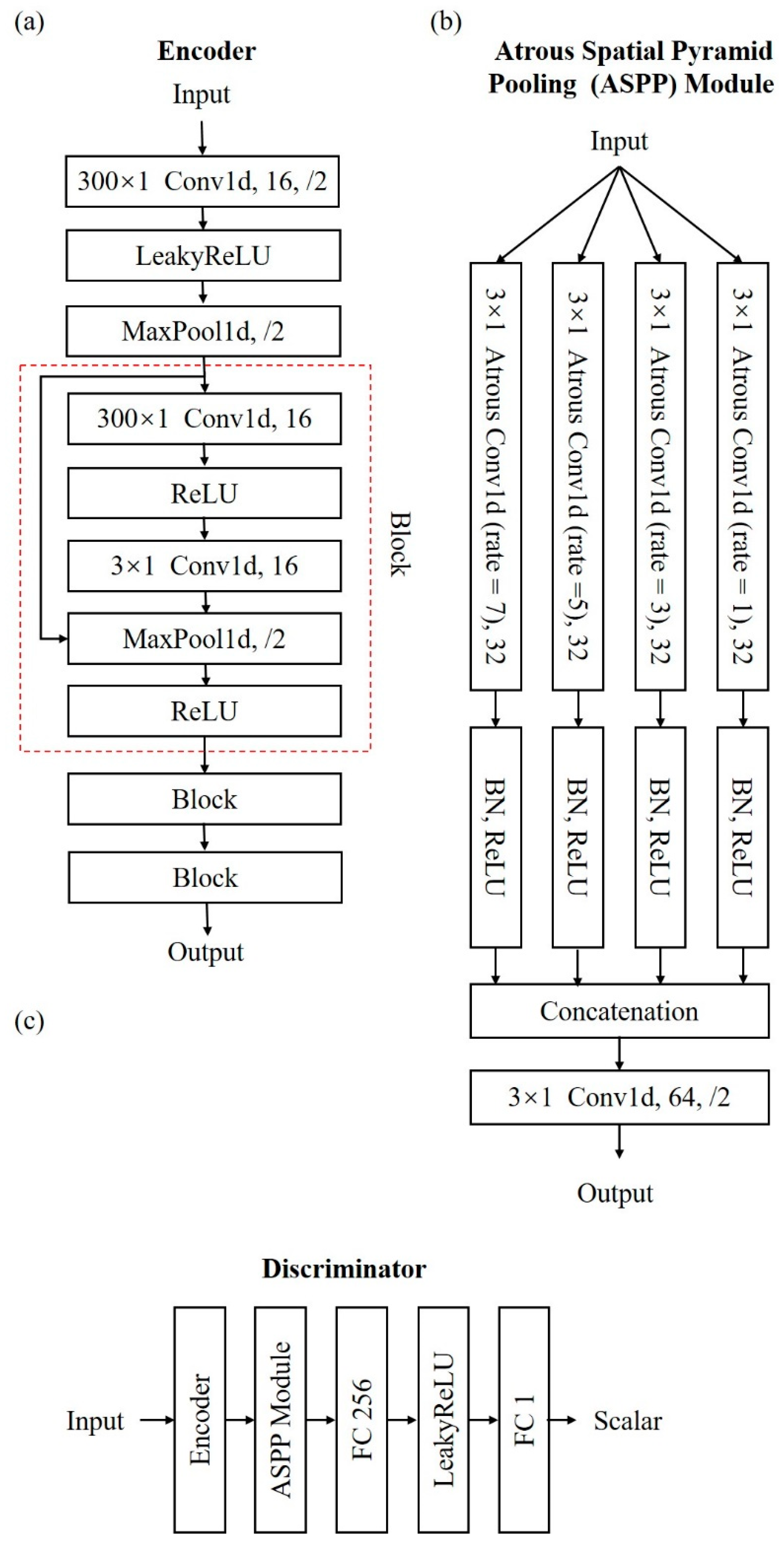
On the other hand, the discriminator is trained to distinguish between the impedance generated by the generator and true impedance from the corresponding seismic traces. The generated impedance or true impedance and the corresponding seismic traces are concatenated together as the input of discriminator. The architecture of the discriminator is illustrated in Figure 2. The discriminator consists of an encoder, an atrous spatial pyramid pooling (ASPP) module and two fully connected layers, which are shown in Figure 2a–c, respectively [40]. The encoder has a similar structure to the generator. We utilize max pooling with stride of 2 in the encoder to downsample the feature maps. ASSP is after the encoder to capture features at multiple scales [40]. In the ASPP module, the resulting feature of four 3 × 1 1D convolutions with dilations of 1, 3, 5, 7 are concatenated. At the end of the discriminator, we use two fully connected layers to output a single scalar.

2.2. Forward Model

We train a CNN as the seismic forward model to learn the synthetic seismic data from impedance, which learns the opposite task to the generator. The architecture of the forward model is same with the generator, as shown in Figure 1. Compared to physical forward operator (i.e., wave theory) [2,3], a deep learning forward model is a generalized form to capture the relationship between data and earth model parameters which may not be described by equations.

2.3. Formulation and Training Details

The forward model F learns the mapping from impedance domain I to seismic domain S . In most seismic exploration, there are limited number of labeled samples from well logs and sufficient unlabeled samples. In this study, we separate the samples into three non-overlapping parts: labeled sample pairs
D l = { ( x l 1 , y l 1 ) , , ( x l N l , y l N l ) | x l i S , y l i I } , unlabeled samples D u = { x u 1 , , x u N u | x u i S } and validation sample pairs D v a l = { ( x v a l 1 , y v a l 1 ) , , ( x v a l N v a l , y v a l N v a l ) | x v a l i S , y v a l i I } . Note that N u N l . The traditional supervised learning is employed to train the forward model F on D l . We use the mean squared error (MSE) loss as the loss function to train F , which can be written as:
L F = E ( x l , y l ) D l [ | | F ( y l ) x l | | 2 2 ]
We obtain F * when the validation loss is minimal in the set epochs. Then, we freeze F * and train the generator and discriminator.
In our method, we introduce the strategies in WGAN-GP into the cGAN framework. Our GAN contains a generator G and a discriminator D . D aims to distinguish between the generated impedance and true impedance under the condition of the corresponding seismic trace. The loss function of D consists of adversarial loss and gradient penalty which is used to enforce the Lipschitz constraint [37]. The loss function of D can be expressed as:
L D = E ( x l , y l ) D l [ D ( x l , y l ) ] + E x l S [ D ( x l , G ( x l ) ) ] Adversarial   loss + λ E x l S [ ( | | y ˜ D ( x l , y ˜ ) | | 2 1 ) 2 ] Gradient   penalty
where y ˜ are randomly sampled points along the straight lines between y l and G ( x l ) , defined by
y ˜ = ϵ y l + ( 1 ϵ ) G ( x l )
where ϵ ~ U [ 0 , 1 ] .   λ is penalty coefficient.
The generator G aims to predict impedance from the input seismic traces. The training of G is supervised by impedance labels and constrained by the forward model F . The loss function of G consists of adversarial loss, impedance loss and seismic loss, which can be formulated as:
L G = E x l S [ D ( x l , G ( x l ) ) ] +   Adversarial   loss α E ( x l , y l ) D l [ | | G ( x l ) y l | | 2 2 ] Impedance   loss + β E x u S [ | | F * ( G ( x u ) ) x u | | 2 2 ] Seismic   loss
where α and β are weights that balance the loss terms. The impedance loss refers to the loss between the generated impedance and the labels and seismic loss is the loss between output of the freezed forward model F * and the unlabeled seimic traces.
All the network parameters are initialized with initialization approach in [41] and trained from scratch with a learning rate of 0.001. Adam optimizer is used in the training with a batch size of 10 [42]. During training, we train D for five steps and then perform one step on G . In the training experiment, the value of adversarial loss is much larger than the value of seismic loss, which makes the seismic loss play a very small role during the training. Therefore, we set large weight coefficients for the seismic loss to balance the adversarial loss and seismic loss. On the other hand, we require more constraints from labeled data than unlabeled data in seismic loss. Thus, we give large weight coefficients to the seismic loss for labeled data constraint. The specific weighting parameters are chosen by trial and error. For all the following experiments in this paper, we set the penalty coefficient λ = 10 in Equation (2) and weights of loss function α = 1000, β = 500 in Equation (4), respectively.

3. Experimental Results, Analysis and Discussion

Marmousi2 model and SEAM model are widely used to validate the performance of deep learning inversion methods [22,26,28]. These two models are used to test the performance of the proposed workflow in seismic impedance inversion in this part first. In addition, we apply the proposed method to the field data to further validate its performance in the last experiment.

3.1. Marmousi2 Model

Marmousi2 P-wave velocity model [43] is an open and generally representative model in the field of geophysics, which has complex stratigraphic structures. The Marmousi2 model is firstly used to validate the proposed method. We calculate reflectivity of this model by using the difference of impedance between two layers, such as the reflectivity of the ith interface of being r i = z i + 1 z i z i + 1 + z i , herein, z i = ρ i v i is the acoustic impedance of the ith layer, ρ i and v i are the density and p-wave velocity of the i th layer, respectively. Seismic data is generated by convoluting the reflectivity with zero-phase Ricker wavelet of 30Hz as shown in Figure 3, in which the abnormal area on the top-left side represents the gas charged sand channel, while the sharp edges and complicated curved interfaces exist on the right side of the profile. The synthetic seismic profile has 13,601 traces with 2800 time points. We choose 101 evenly-spaced traces from the seismic and impedance profile as labeled data denoted by D l ( N l = 101), which is less than 1% of the total traces. For the rest 13,500 traces, we randomly select 10% (1350 sample pairs) as D v a l   ( N v a l   = 1350) and 90% seismic traces as D u   ( N u   = 12,150).
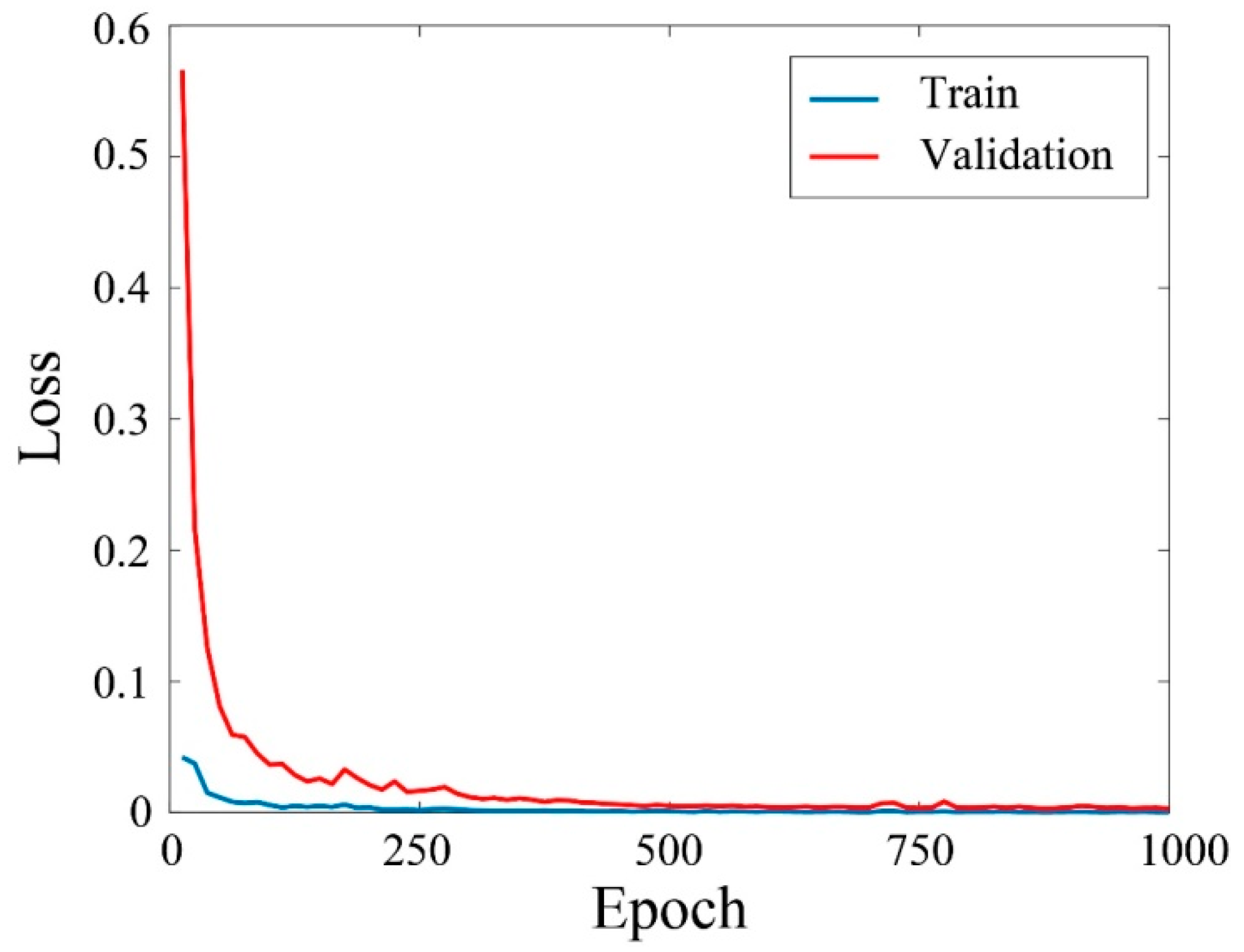
In our framework, we first train the forward model F on D l to synthesize seismic traces from impedance. Then, we freeze the forward model F * after 1000 epochs training as the network converges in 1000 epochs and we obtain F * when the validation loss is minimal. The training and validation convergence curves is illustrated in Figure 4. Subsequently, we train D and G to minimize L D and L G in Equations (2) and (4) for 1000 epochs. After the entire training procedure, the generator G is utilized to predict impedance from seismic data. To show the performance of the proposed method compared to conventional deep learning inversion methods in the case of limited labeled data, we choose a conventional CNN method as baseline. The CNN has the same architecture as that of the generator as well as forward model and it is trained with supervised learning on D l to minimize the MSE between the predicted impedance and labels. The training details of CNN and the forward model are exactly the same.
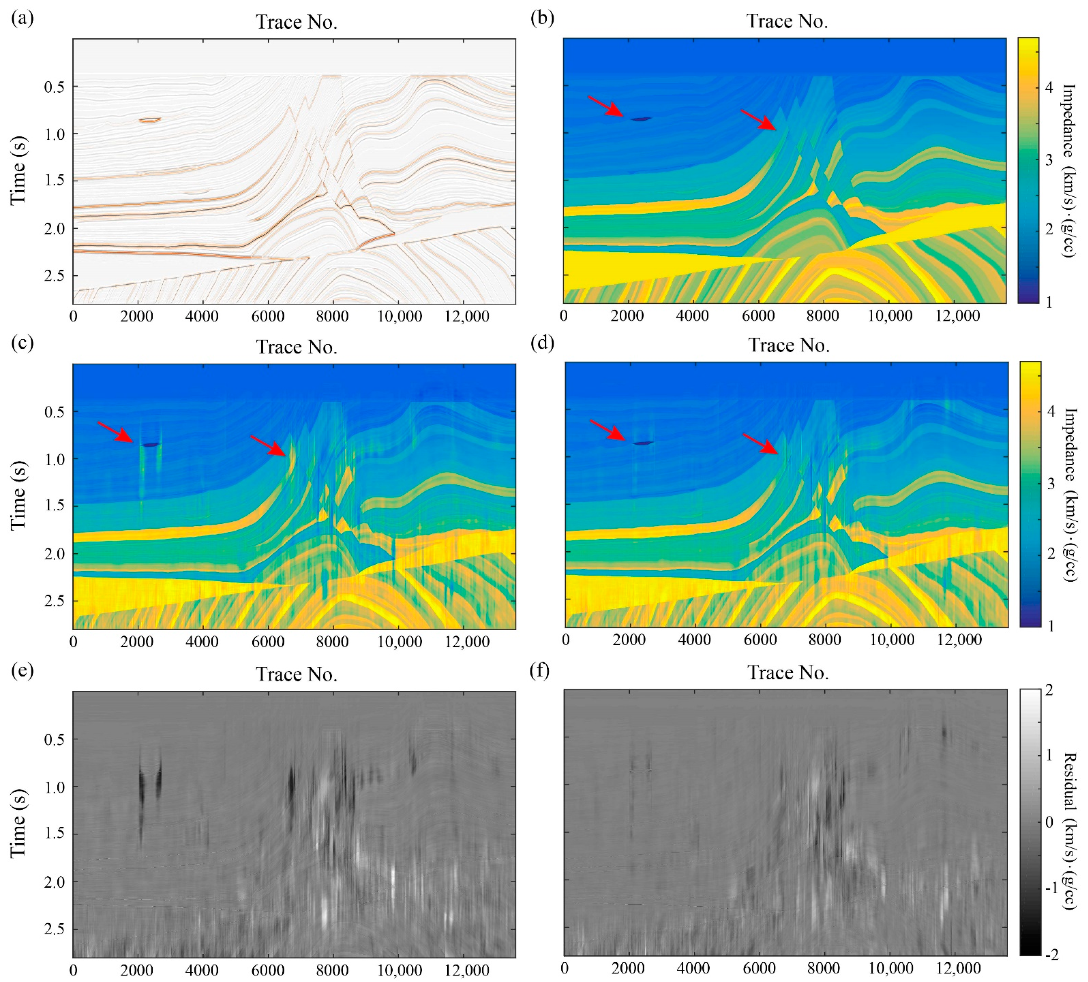
We first show the seismic section predicted by the forward model F * in Figure 5a. The predicted seismic section is highly consistent with true seismic section compared to Figure 3 with metrics: average r 2 coefficient of being 0.9903, Pearson’s Correlation Coefficient (PCC) of being 0.9955 and MSE of being 9.544 × 10 6 , respectively. The impedance profiles predicted by conventional CNN method and our method are illustrated in Figure 5c,d, respectively. The true impedance profile and the residual profiles are also respectively shown in Figure 5b,e,f for comparison. It can be seen that the impedance predicted by our method is closer to the true impedance than that of CNN, especially for the gas charged sand channel and the area of complex structures indicated by red arrows. Figure 5 obviously indicates that the proposed method improves the result on CNN around the edges of the abnormal region and the complex structures. The average r 2 coefficient, PCC and MSE between the predicted impedance profiles and true impedance are also calculated and shown in Table 1. All the metrics of our method are better than those of the CNN method, which demonstrates the effectiveness of the proposed method.
In addition, the impedance of Marmousi2 model around the area of the gas charged sand channel and complex structure marked by the red arrows in Figure 5 are more difficult to be estimated. The prediction of impedance from those areas are challenging for the conventional CNN method due to the lack of labeled training data. We choose two highly representative traces with Trace No. 2700 and 7440, which belong to D v a l , to show the performance of our method by comparing with the result of CNN as illustrated in Figure 6. Figure 6a,b show the variations of impedance with respect to time for the Trace No. 2700 and Trace No. 7440, respectively. The red line, green line and blue line respectively refer to the true impedance, impedance predicted by CNN and the proposed method. The Trace No. 2700 is next to the right border of the channel, where a sudden transition of impedance occurs, while the Trace No. 7440 passes through most layers of the profile incorporating complicated structures such as sharp edges. Figure 6 indicates that the impedance predicted by our method basically matches well with the true values of impedance for both traces. The prediction of CNN largely deviates from the true impedance at the time range of 0.7 s to 1.2 s for Trace No. 2700 and the time after 0.7 s for the Trace No. 7440. It is noted that the large deviation from CNN respectively occurs at the area of the gas charged sand channel for Trace No. 2700 and the appearance of sharp edges for Trace No. 7440. The PCC of the proposed method on Trace No. 2700 and No. 7440 are 0.9970 and 0.9880, respectively, while those of CNN method are 0.9384 and 0.8855 respectively. Hence, the proposed method predicts more accurate impedance than that of the conventional CNN. The improvement of our method is mainly contributed by the utilization of the unlabeled data during training.

3.2. SEAM Model

In order to further validate the feasibility of our method, we conduct our workflow on another dataset, SEAM, which is open and also widely used for the validation of deep learning inversion methods [16,29,44]. The SEAM model is a 3-D seismic survey with strong lateral varying density and p-wave velocity which is challenging for inversion algorithms. A 2-D cross-section impedance is used in our tests, which is obtained by the multiplication of density and p-wave velocity. The selected 2-D profile as illustrated in Figure 7, which has 1751 traces with 2501 time points and the time interval is 8ms. We choose 34 evenly-spaced traces (1.94%) as D l . The proportion of labeled data is less than that in [16,44]. For the other 1719 traces, we randomly choose 171 traces (10%) as D v a l and 1546 traces (90%) as D u . We train the network with the same way as that in the Marmousi2 model, then we perform impedance inversion over all 2-D profile with the trained network. Figure 7 shows the true impedance section (Figure 7a), the impedance predicted by the aforementioned CNN method (Figure 7b) and the impedance predicted by our method (Figure 7c). It can be seen that our method gives a better prediction than the CNN method. Furthermore, we compute the average r 2 coefficient and PCC over all the impedance pseudo-wells (1751 traces) in the seismic section to quantitatively evaluate the performance of the proposed method, as shown in Table 2. Table 2 lists the result of our method with those of the state-of-the-art deep learning inversion methods. Table 2 clearly indicates that the values of PCC and r 2 of our method are, respectively, 0.9902 and 0.9753, which are larger than that of other methods such as CNN (0.9770, 0.9436), joint learning 2-D TCN (unavailable, 0.8399) [16], 2-D TCN (0.9259, 0.7977) [44], 1-D TCN (0.9088, 0.6709) [26] and LSTM (0.8526, 0.4738) [44].
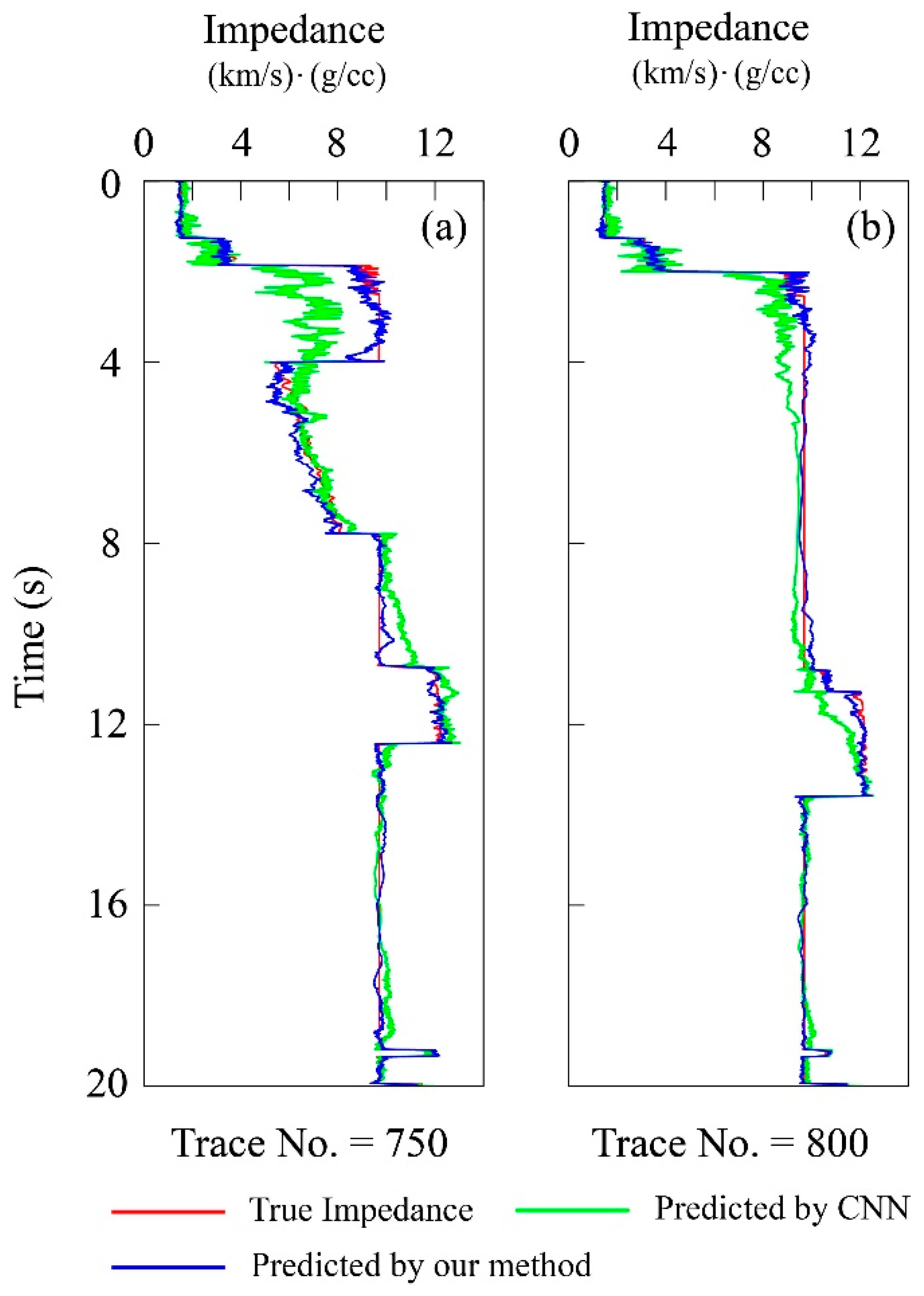
In order to demonstrate the effectiveness of the proposed method in the complicated SEAM model, we select two representative traces such as Trace No. 750 and Trace No. 800 as marked with red dashed line in Figure 7a to clearly show the details of prediction. Trace No. 750 is located in the most complex part of the SEAM model, which passes through the low-velocity zone between layers with high velocities and the deeper layer of Trace No. 750 is incorporated with rugged salt interfaces. Trace No. 800 is located in the relatively simple area of the model, which pass the whole area of the salt body. Figure 8a,b illustrates the variations of impedance prediction of CNN method (green line) and the proposed method (blue line) with respect to time for the Trace No. 750 and Trace No. 800 and the true impedance (red line) is also shown in those figures for comparison. The PCC of the proposed method on Trace No. 750 and No. 800 are 0.9948 and 0.9977, respectively, while those of CNN method are 0.9256 and 0.9834 respectively. Figure 8 clearly indicates that the impedance predicated with the presented method matches well with the true values through the whole shallow to deeper layers. Especially, the prediction of our method at the low-velocity zone for the Trace No. 750 displays a consistent result with true impedance. These detailed results further prove the performance of our method.

3.3. Volve Field Data

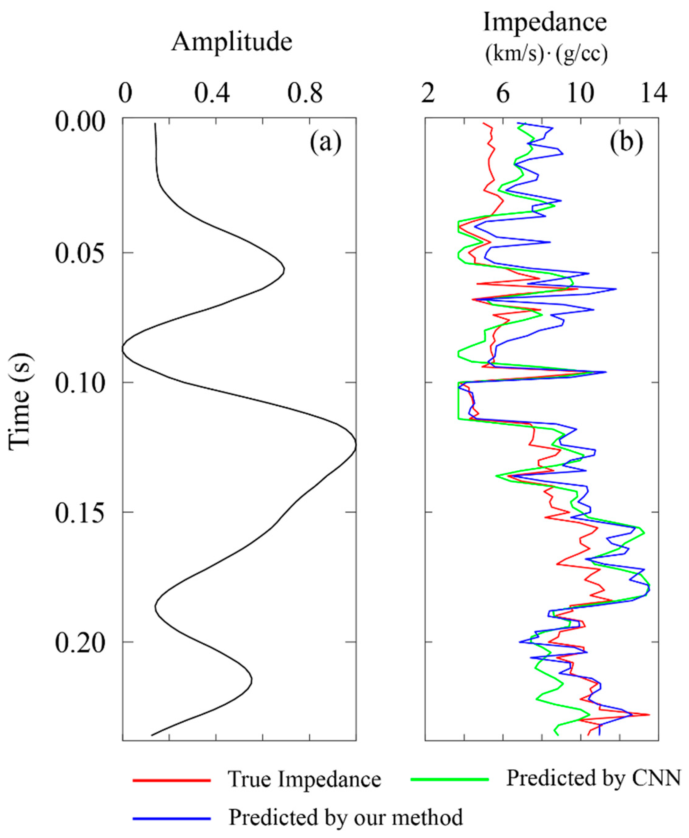
We use Volve field data to validate the effectiveness of the proposed method. The Volve field, a clastic reservoir, is located in offshore Norway as illustrated in Figure 9. We obtain the dataset from the open source code of [25]. The dataset has 1300 impedance traces, which are generated based on the statistics of the impedance log from the well location as shown in Figure 9b using the data augmentation method [25]. We randomly choose 750 traces as labeled training data D l , which is the same as [25]. For the rest of 550 traces, we randomly choose half (275 traces) of them as D u and the other half is used as D v a l . In this experiment, we change all the kernels with size 300 to size 80 in all the networks in our method, because the data only has 160 time points in this experiment. We then followed proposed workflow to train the networks and invert the impedance at the well location. Figure 10a shows the input seismic data along the well as illustrated in Figure 9b. Figure 10b compares the impedance predicted by our method (blue line) with that of the CNN method (green line) [25] and the true impedance at the well location is also shown in Figure 10 (red line). In general, there are good sides for results of both CNN and the proposed method. At the very beginning (around 0.01 s) and time interval between 0.06 s and 0.07 s, CNN shows better result while the proposed method behaves a good match with the true impedance for the time span after 0.2 s. However, the PCC of our method is 0.88 which is higher than that of CNN being 0.82. Furthermore, we repeated the Volve data experiment for five times to show the influence of random samples on the results. Each time, we randomly choose the training samples accordingly mentioned above. The PCCs of these five times are 0.8772, 0.8895, 0.8656, 0.8791, 0.8939 respectively and aforementioned 0.88 is the average. The result of the Volve field data proves effectiveness of the proposed method on real scenario.

3.4. Discussion

The proposed workflow includes three networks, a generator, a discriminator and a forward network. The generator and forward network share same architecture as fully convolutional residual network (FCRN) in [12] and only small adjustment is made to fit into the WGAN-GP framework. For example, the kernel size we used is 300, which is same as [12,25,28]. We did not conduct ablation study to show the superiority of the chosen hyperparameters. For sure there would be network module or architecture with higher accuracy or efficiency to improve the proposed method. Our preliminary tests show that dilated convolution [45], with same receptive field as the original kernel and appropriate dilation value in suitable position, can dramatically reduce the number of network parameters but producing a higher accurate result. Comparing to the supervised network with same prediction result in Figure 4, the training time of the proposed algorithm almost quadrupled since there are three networks to train and more loss terms to calculate. However, the prediction efficiency is the same because only the trained generator is used after training process. For the synthetic tests, the wavelet is the same for all time and locations, which is not a premise for the field data prediction. To avoid the wavelet time varying effect, for the Volve field data prediction, only a short time span of seismic data (0.236 s) is used for the tests. Only one-shot impedance prediction is given for the proposed workflow. It is necessary to quantify the uncertainty of the prediction for quantitative geoscientific interpretation or inversion. Das et al. proposed to use approximate Bayesian computation (ABC) for the posterior uncertainty quantification [25]. The uncertainty estimation in impedance inversion can be achieved using Bayesian deep learning [46]. Bayesian models offer grounded mathematical foundation but with prohibitive computation cost. The regression results uncertainty from generator, also known as epistemic uncertainty, can be estimated by the Monte Carlo dropout Bayesian approach [47]. A dropout layer can be added after the convolution layer in the generator. In the prediction stage, multiple Monte Carlo samples can be retrieved due to different weights from the dropout layer for different execution [48]. This is one of the research topics for impedance estimation currently and also for the future.

4. Conclusions

We propose a semi-supervised learning workflow based on GAN for seismic impedance inversion. The GAN-based network is composed of a forward model, a generator and a discriminator, in which the CNN is trained as a forward model to learn seismic data from impedance. In this way, the forward model is a data-driven model that can better capture the geophysical feature of the training data by comparing with the traditional forward operator such as convolutional model. The generator in GAN is trained to predict impedance from the input seismic data by minimizing adversarial loss and seismic loss which make uses of both labeled and unlabeled data. We introduce the strategies in WGAN-GP into the cGAN framework. The process of training generator is supervised by the labeled data and constrained by the forward model. The discriminator is trained to distinguish between the generated impedance and true impedance corresponding to the input seismic traces as accurately as possible through minimizing the adversarial loss and gradient penalty loss. The gradient penalty is introduced to enforce the Lipschitz constraint in the training of the discriminator. Tests on Marmousi2 model and SEAM model show that the proposed method predicts more accurate impedance than that of the conventional CNN and other state-of-the-art deep learning inversion methods. The test results show that the proposed workflow outperforms the conventional CNN method in Marmousi2 model especially in challenging areas and the performance metrics are improved in SEAM model. In addition, the field data are also applied to demonstrate the performance of the proposed method, the result indicates that the presented method improves the prediction of CNN.

Author Contributions

All the authors made significant contributions to this work. B.W. and D.M. designed the framework of the network and performed the experiments; H.Z. and B.W. analyzed the results; H.Z. and D.M. wrote the paper; H.Z. and B.W. acquired the funding support. All authors have read and agreed to the published version of the manuscript.

Funding

This research was funded by the National Natural Science Foundation of China under Grants 41974132, 41504091 and 41974122, by Natural Science Basic Research Program of Shaanxi Program under Grant 2020JM-018, by Fundamental Research Funds for the Central Universities under Grant xjj2018260.

Institutional Review Board Statement

Not applicable.

Informed Consent Statement

Not applicable.

Data Availability Statement

The data for Marmousi2 Model and SEAM model are obtained from https://wiki.seg.org/wiki/Open_data#SEAM_open_data (accessed on 30 December 2020), the Volve field data is obtained from https://github.com/vishaldas/CNN_based_impedance_inversion/tree/master/Volve_field_example (accessed on 30 December 2020).

Acknowledgments

The authors would like to thank SEG and GARY S. MARTIN et al. for the two open models: Marmousi2 and SEAM model, Vishal Das et al. for the open source code and prediction results of Volve field data. We also thank Qiao Xie for conducting the dilated convolution tests for the CNN impedance inversion. We are thankful to the editors and the three anonymous reviewers for their constructive comments and suggestions that significantly improve the quality of the manuscript.

Conflicts of Interest

The authors declare no conflict of interest.

References

  1. Tarantola, A. A Strategy for nonlinear elastic inversion of seismic-reflection data. Geophysics 1986, 51, 1893–1903. [Google Scholar] [CrossRef]
  2. Buland, A.; More, H. Bayesian linearized AVO inversion. Geophysics 2003, 68, 185–198. [Google Scholar] [CrossRef] [Green Version]
  3. Virieux, J.; Operto, S. An overview of full-waveform inversion in exploration geophysics. Geophysics 2009, 74, WCC1–WCC26. [Google Scholar] [CrossRef]
  4. Yang, H.; Jia, J.; Wu, B.; Gao, J. Mini-batch optimized full waveform inversion with geological constrained gradient filtering. J. Appl. Geophys. 2018, 152, 9–16. [Google Scholar] [CrossRef]
  5. Sun, M.; Jin, S. Multiparameter Elastic Full Waveform Inversion of Ocean Bottom Seismic Four-Component Data Based on A Modified Acoustic-Elastic Coupled Equation. Remote Sens. 2020, 12, 2816. [Google Scholar] [CrossRef]
  6. Duijndam, A.J.W. Bayesian-estimation in seismic inversion: 1. Principles. Geophys. Prospect. 1988, 36, 878–898. [Google Scholar] [CrossRef]
  7. Gholami, A. Nonlinear multichannel impedance inversion by total-variation regularization. Geophysics 2015, 80, R217–R224. [Google Scholar] [CrossRef]
  8. Huang, W.-L.; Gao, F.; Liao, J.-P.; Chuai, X.-Y. A deep learning network for estimation of seismic local slopes. Pet. Sci. 2021, 18, 92–105. [Google Scholar] [CrossRef]
  9. Zhang, Z.-D.; Alkhalifah, T. Regularized elastic full-waveform inversion using deep learning. Geophysics 2019, 84, R741–R751. [Google Scholar] [CrossRef]
  10. Wang, Y.; Ge, Q.; Lu, W.; Yan, X. Seismic impedance inversion based on cycle-consistent generative adversarial network. In SEG Technical Program Expanded Abstracts 2019; Society of Exploration Geophysicists: Tulsa, OK, USA, 2019; pp. 2498–2502. [Google Scholar] [CrossRef]
  11. Zhang, Z.; Lin, Y. Data-Driven Seismic Waveform Inversion: A Study on the Robustness and Generalization. IEEE Trans. Geosci. Remote. Sens. 2020, 58, 6900–6913. [Google Scholar] [CrossRef] [Green Version]
  12. Wu, B.; Meng, D.; Wang, L.; Liu, N.; Wang, Y. Seismic Impedance Inversion Using Fully Convolutional Residual Network and Transfer Learning. IEEE Geosci. Remote Sens. Lett. 2020, 17, 2140–2144. [Google Scholar] [CrossRef]
  13. Wang, Y.; Ge, Q.; Lu, W.; Yan, X. Well-Logging Constrained Seismic Inversion Based on Closed-Loop Convolutional Neural Network. IEEE Trans. Geosci. Remote Sens. 2020, 58, 5564–5574. [Google Scholar] [CrossRef]
  14. Pan, W.; Torres-Verdin, C.; Pyrcz, M.J. Stochastic Pix2pix: A New Machine Learning Method for Geophysical and Well Conditioning of Rule-Based Channel Reservoir Models. Nat. Resour. Res. 2020. [Google Scholar] [CrossRef]
  15. Jo, H.; Santos, J.E.; Pyrcz, M.J. Conditioning well data to rule-based lobe model by machine learning with a generative adversarial network. Energy Explor. Exploit. 2020, 38, 2558–2578. [Google Scholar] [CrossRef]
  16. Mustafa, A.; AlRegib, G. Joint learning for seismic inversion: An acoustic impedance estimation case study. In SEG Technical Program Expanded Abstracts 2020; Society of Exploration Geophysicists: Tulsa, OK, USA, 2020; pp. 1686–1690. [Google Scholar] [CrossRef]
  17. Li, S.; Liu, B.; Ren, Y.; Chen, Y.; Yang, S.; Wang, Y.; Jiang, P. Deep-Learning Inversion of Seismic Data. IEEE Trans. Geosci. Remote Sens. 2020, 58, 2135–2149. [Google Scholar] [CrossRef] [Green Version]
  18. Wang, B.; Zhang, N.; Lu, W.; Wang, J. Deep-learning-based seismic data interpolation: A preliminary result. Geophysics 2019, 84, V11–V20. [Google Scholar] [CrossRef]
  19. Huang, W. Seismic signal recognition by unsupervised machine learning. Geophys. J. Int. 2019, 219, 1163–1180. [Google Scholar] [CrossRef]
  20. Liu, N.; He, T.; Tian, Y.; Wu, B.; Xu, Z. Common azimuth seismic data fault analysis using residual U-Net. Interpretation 2020, 8, 1–41. [Google Scholar] [CrossRef]
  21. Wang, Z.; Li, B.; Liu, N.; Wu, B.; Zhu, X. Distilling knowledge from an ensemble of convolutional neural networks for seismic fault detection. IEEE Geosci. Remote Sens. Lett. 2020, 1–5. [Google Scholar] [CrossRef]
  22. Qiu, C.; Wu, B.; Liu, N.; Zhu, X.; Ren, H. Deep Learning Prior Model for Unsupervised Seismic Data Random Noise Attenuation. IEEE Geosci. Remote Sens. Lett. 2021, 1–5. [Google Scholar] [CrossRef]
  23. Kim, Y.; Nakata, N. Geophysical inversion versus machine learning in inverse problems. Lead. Edge 2018, 37, 894–901. [Google Scholar] [CrossRef]
  24. Alfarraj, M.; AlRegib, G. Petrophysical property estimation from seismic data using recurrent neural networks. In SEG Technical Program Expanded Abstracts 2018; Society of Exploration Geophysicists: Tulsa, OK, USA, 2018; pp. 2141–2146. [Google Scholar] [CrossRef]
  25. Das, V.; Pollack, A.; Wollner, U.; Mukerji, T. Convolutional neural network for seismic impedance inversion. Geophysics 2019, 84, R869–R880. [Google Scholar] [CrossRef]
  26. Mustafa, A.; Alfarraj, M.; AlRegib, G. Estimation of acoustic impedance from seismic data using temporal convolutional network. In EG Technical Program Expanded Abstracts 2019; Society of Exploration Geophysicists: Tulsa, OK, USA, 2019; pp. 2554–2558. [Google Scholar] [CrossRef] [Green Version]
  27. Du, J.; Liu, J.; Zhang, G.; Han, L.; Li, N. Pre-stack seismic inversion using SeiInv-ResNet. In EG Technical Program Expanded Abstracts 2019; Society of Exploration Geophysicists: Tulsa, OK, USA, 2019; pp. 2338–2342. [Google Scholar] [CrossRef]
  28. Alfarraj, M.; Alregib, G. Semi-supervised Sequence Modeling for Elastic Impedance Inversion. Interpretation 2019, 7, SE237–SE249. [Google Scholar] [CrossRef]
  29. Cai, A.; Di, H.; Li, Z.; Maniar, H.; Abubakar, A. Wasserstein cycle-consistent generative adversarial network for improved seismic impedance inversion: Example on 3D SEAM model. In SEG Technical Program Expanded Abstracts 2020; Society of Exploration Geophysicists: Tulsa, OK, USA, 2020; pp. 1274–1278. [Google Scholar] [CrossRef]
  30. Goodfellow, I.; Pouget-Abadie, J.; Mirza, M.; Xu, B.; Warde-Farley, D.; Ozair, S.; Courville, A.; Bengio, Y. Generative adversarial nets. In Proceedings of the Advances in Neural Information Processing Systems, Montréal, QC, Canada, 8–13 December 2014; pp. 2672–2680. [Google Scholar]
  31. Denton, E.L.; Chintala, S.; Szlam, A.; Fergus, R. Deep generative image models using a Laplacian pyramid of adversarial networks. In Proceedings of the Advances in Neural Information Processing Systems (NIPS), Montreal, QC, Canada, 7–12 December 2015; pp. 1486–1494. [Google Scholar]
  32. Radford, A.; Metz, L.; Chintala, S. Unsupervised representation learning with deep convolutional generative adversarial networks. arXiv 2015, arXiv:1511.06434. [Google Scholar]
  33. Kaur, H.; Pham, N.; Fomel, S. Seismic data interpolation using CycleGAN. In SEG Technical Program Expanded Abstracts 2019; Society of Exploration Geophysicists: Tulsa, OK, USA, 2019; pp. 2202–2206. [Google Scholar] [CrossRef]
  34. Li, Q.; Luo, Y. Using GAN priors for ultrahigh resolution seismic inversion. In SEG Technical Program Expanded Abstracts 2019; Society of Exploration Geophysicists: Tulsa, OK, USA, 2019; pp. 2453–2457. [Google Scholar] [CrossRef]
  35. Mirza, M.; Osindero, S. Conditional generative adversarial nets. arXiv 2014, arXiv:1411.1784. [Google Scholar]
  36. Arjovsky, M.; Chintala, S.; Bottou, L. Wasserstein GAN. 2017. arXiv 2017, arXiv:1701.07875. [Google Scholar]
  37. Gulrajani, I.; Ahmed, F.; Arjovsky, M.; Dumoulin, V.; Courville, A.C. Improved training of wasserstein gans. In Advances in Neural Information Processing Systems; MIT Press: Cambridge, MA, USA, 2017; pp. 5767–5777. [Google Scholar]
  38. Krizhevsky, A.; Sutskever, I.; Hinton, G.E. ImageNet Classification with Deep Convolutional Neural Networks. Commun. ACM 2017, 60, 84–90. [Google Scholar] [CrossRef]
  39. Ioffe, S.; Szegedy, C. Batch Normalization: Accelerating Deep Network Training by Reducing Internal Covariate Shift. arXiv 2015, arXiv:1502.03167. [Google Scholar]
  40. Chen, L.-C.; Papandreou, G.; Kokkinos, I.; Murphy, K.; Yuille, A.L. DeepLab: Semantic Image Segmentation with Deep Convolutional Nets, Atrous Convolution, and Fully Connected CRFs. IEEE Trans. Pattern Anal. Mach. Intell. 2018, 40, 834–848. [Google Scholar] [CrossRef]
  41. He, K.; Zhang, X.; Ren, S.; Sun, J. Delving deep into rectifiers: Surpassing human-level performance on ImageNet classification. In Proceedings of the IEEE International Conference on Computer Vision, Las Condes, Chile, 11–18 December 2015; pp. 1026–1034. [Google Scholar]
  42. Kingma, D.; Ba, J. Adam: A Method for Stochastic Optimization. arXiv 2014, arXiv:1412.6980. [Google Scholar]
  43. Martin, G.S.; Wiley, R.; Marfurt, K.J. Marmousi2: An elastic upgrade for Marmousi. Lead. Edge 2006, 25, 156–166. [Google Scholar] [CrossRef]
  44. Mustafa, A.; Alfarraj, M.; AlRegib, G. Spatiotemporal modeling of seismic images for acoustic impedance estimation. In SEG Technical Program Expanded Abstracts 2020; Society of Exploration Geophysicists: Tulsa, OK, USA, 2020; pp. 1735–1739. [Google Scholar] [CrossRef]
  45. Yu, F.; Koltun, V. Multi-Scale Context Aggregation by Dilated Convolutions. ICLR arXiv 2016, arXiv:1511.07122v3. [Google Scholar]
  46. Junhwan, C.; Dowan, K.; Joongmoo, B. Uncertainty estimation in impedance inversion using Bayesian deep learning. In SEG Technical Program Expanded Abstracts 2020; Society of Exploration Geophysicists: Tulsa, OK, USA, 2020; pp. 3887–3891. [Google Scholar] [CrossRef]
  47. Kendall, A.; Gal, Y. What Uncertainties Do We Need in Bayesian Deep Learning for Computer Vision? arXiv 2017, arXiv:1703.04977. [Google Scholar]
  48. Zhao, T.; Chen, X. Enrich the interpretation of seismic image segmentation by estimating epistemic uncertainty. In SEG Technical Program Expanded Abstracts 2020; Society of Exploration Geophysicists: Tulsa, OK, USA, 2020. [Google Scholar] [CrossRef]
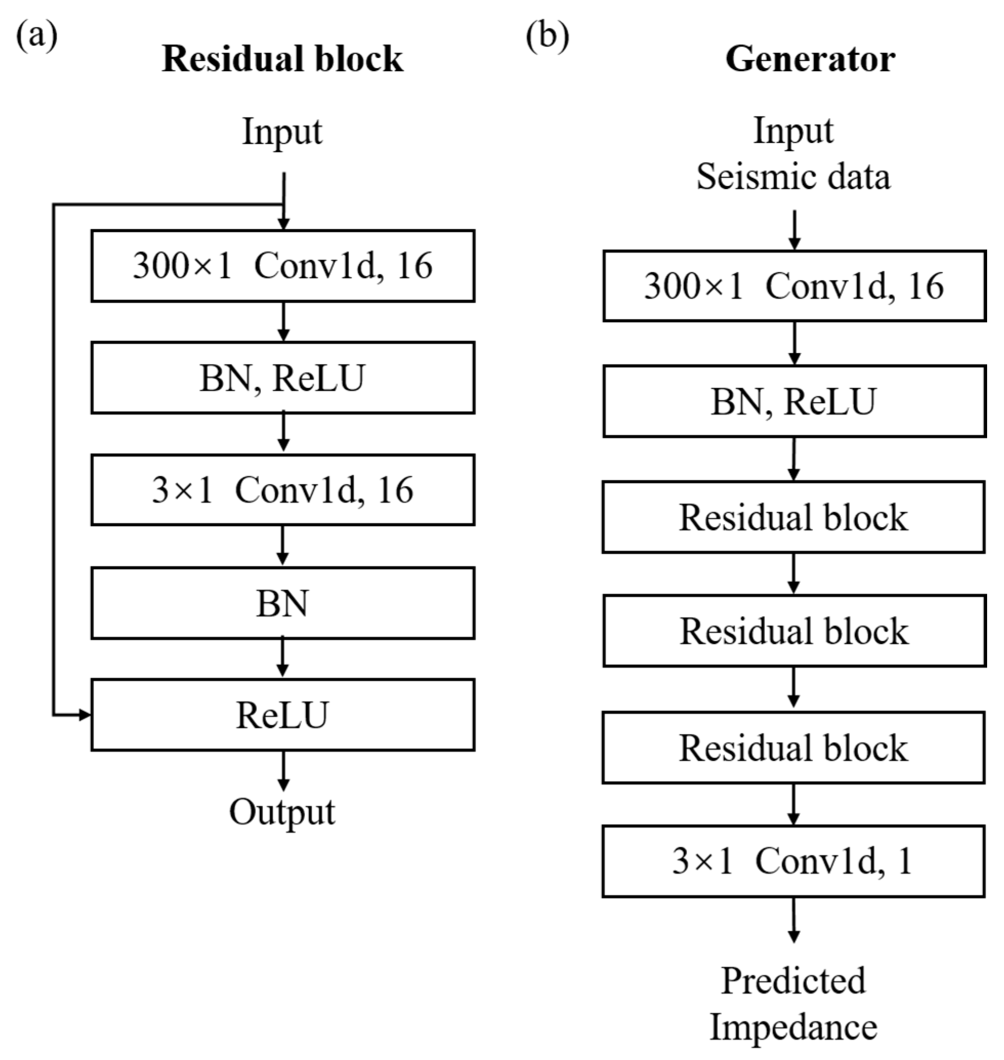
Figure 1. The architecture of the (a) residual block and (b) generator.
Remotesensing 13 00909 g001
Figure 2. The architecture of (a) encoder, (b) Atrous spatial pyramid pooling (ASPP) module and (c) discriminator.
Remotesensing 13 00909 g002
Figure 3. Synthetic seismic data profile of Marmousi2.
Remotesensing 13 00909 g003
Figure 4. The training and validation convergence curves on Marmousi2 model.
Remotesensing 13 00909 g004
Figure 5. Predicted seismic data section, impedance sections, true impedance section and residual sections on Marmousi2 model: (a) the seismic data section predicted by the forward model F * ; (b) the true impedance; (c) the impedance predicted by conventional Convolutional Neural Network (CNN) method; (d) the impedance predicted by the proposed method; (e) the residual of (c,b); (f) the residual of (d,b). The red arrows mark the abnormal gas charged sand channel and the complex structures in the model.
Remotesensing 13 00909 g005
Figure 6. Impedance of the selected representative traces. (a) Trace number: 2700; (b) Trace number: 7440.
Remotesensing 13 00909 g006
Figure 7. Predicted impedance and true impedance of SEAM model: (a) true impedance; (b) impedance predicted CNN method; (c) impedance predicted by proposed method.
Remotesensing 13 00909 g007
Figure 8. Impedance of the selected representative traces. (a) Trace number: 750; (b) Trace number: 800.
Remotesensing 13 00909 g008
Figure 9. (a) Volve field shown in map located in offshore North Sea, (b) Seismic data along with a well trajectory from the Volve field (Figures are from [25]).
Remotesensing 13 00909 g009
Figure 10. (a) Input seismic data along well and (b) true impedance (red line), impedance predicted by CNN (green line) and our method (blue line) along the well. The correlation between true impedance and impedance predicted by our method is 0.88 which is higher than 0.82 in [25].
Remotesensing 13 00909 g010
Table 1. Performance metrics of our method on Marmousi2 model compared with the conventional CNN method.
MetricOur MethodCNN
MSE0.01840.0332
PCC0.99480.9938
r 2 0.98740.9847
Table 2. Performance metrics of our method on a section of SEAM model compared with that of the state-of-the-art deep learning inversion methods.
MetricOur MethodCNNJoint Learning 2-D TCN [16]2-D TCN [44]1-D TCN [26]LSTM [44]
PCC0.99020.9770unavailable0.92590.90880.8526
r 2 0.97530.94360.83990.79770.67090.4738
Publisher’s Note: MDPI stays neutral with regard to jurisdictional claims in published maps and institutional affiliations.