
Performance Comparison of Machine Learning Models for Annual Precipitation Prediction Using Different Decomposition Methods


Abstract
1. Introduction
2. Method
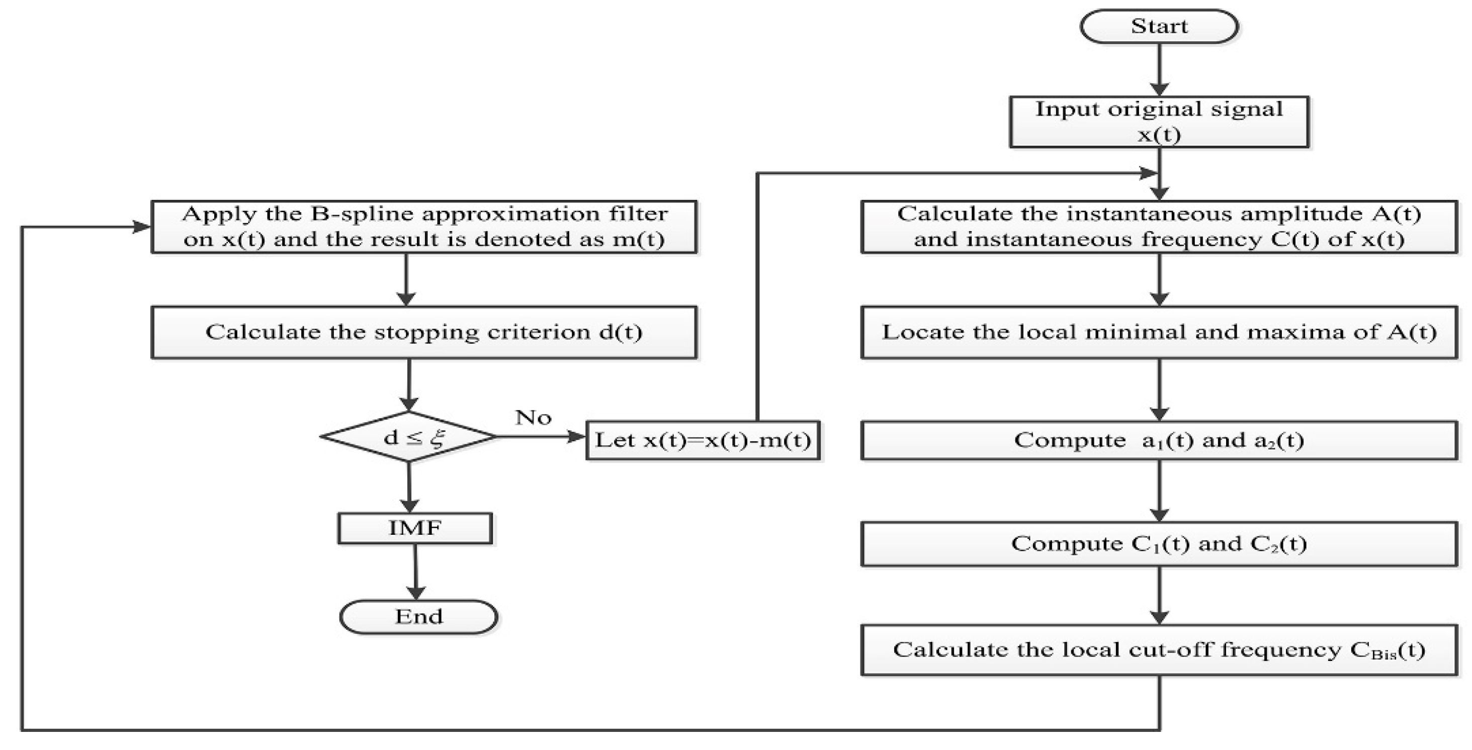
2.1. Time-Varying Filter-Based EMD

2.2. REMD Decomposition Method
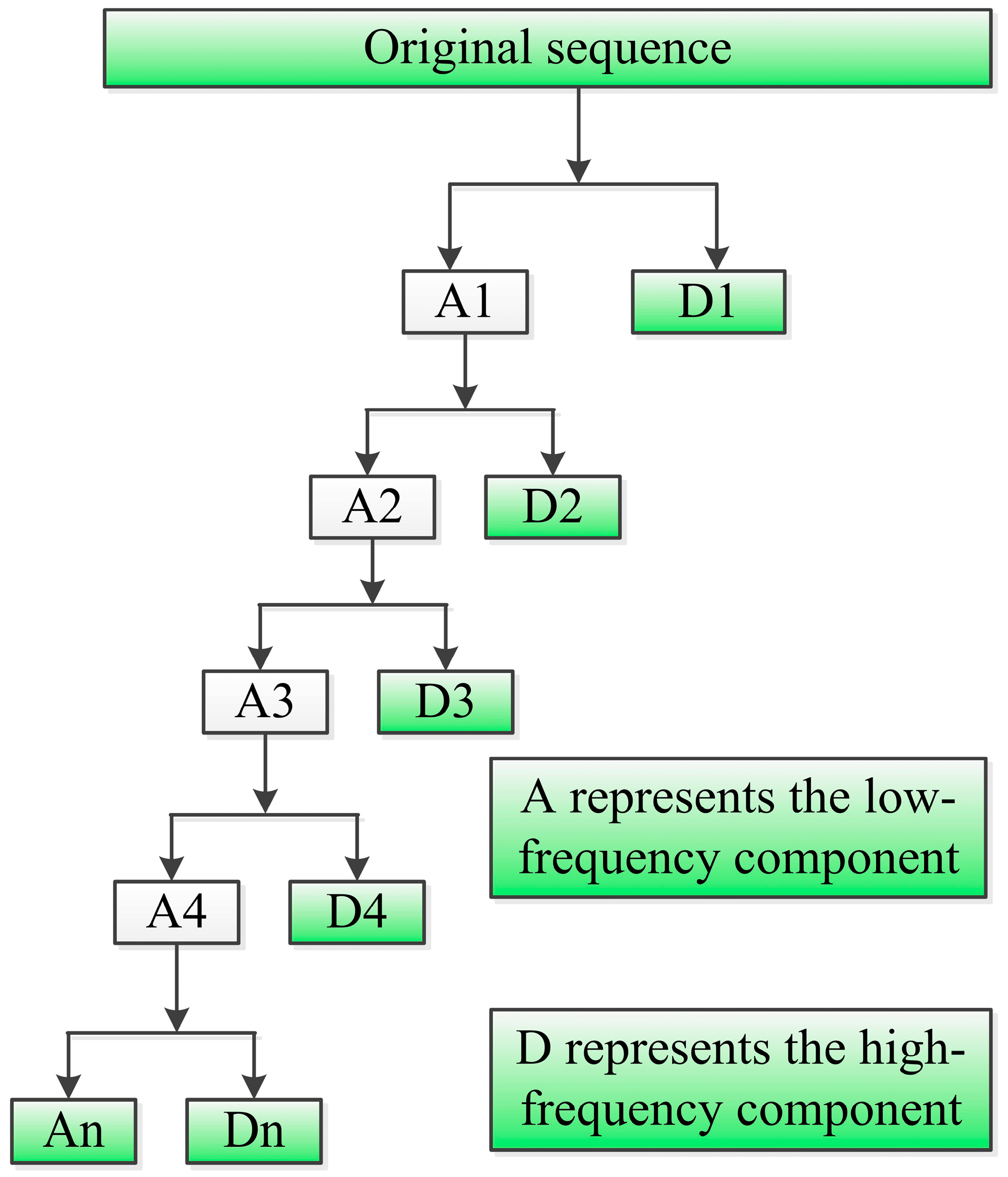
2.3. Complementary Ensemble Empirical Mode Decomposition
2.4. Wavelet Transform
2.5. Extreme-Point Symmetric Mode Decomposition
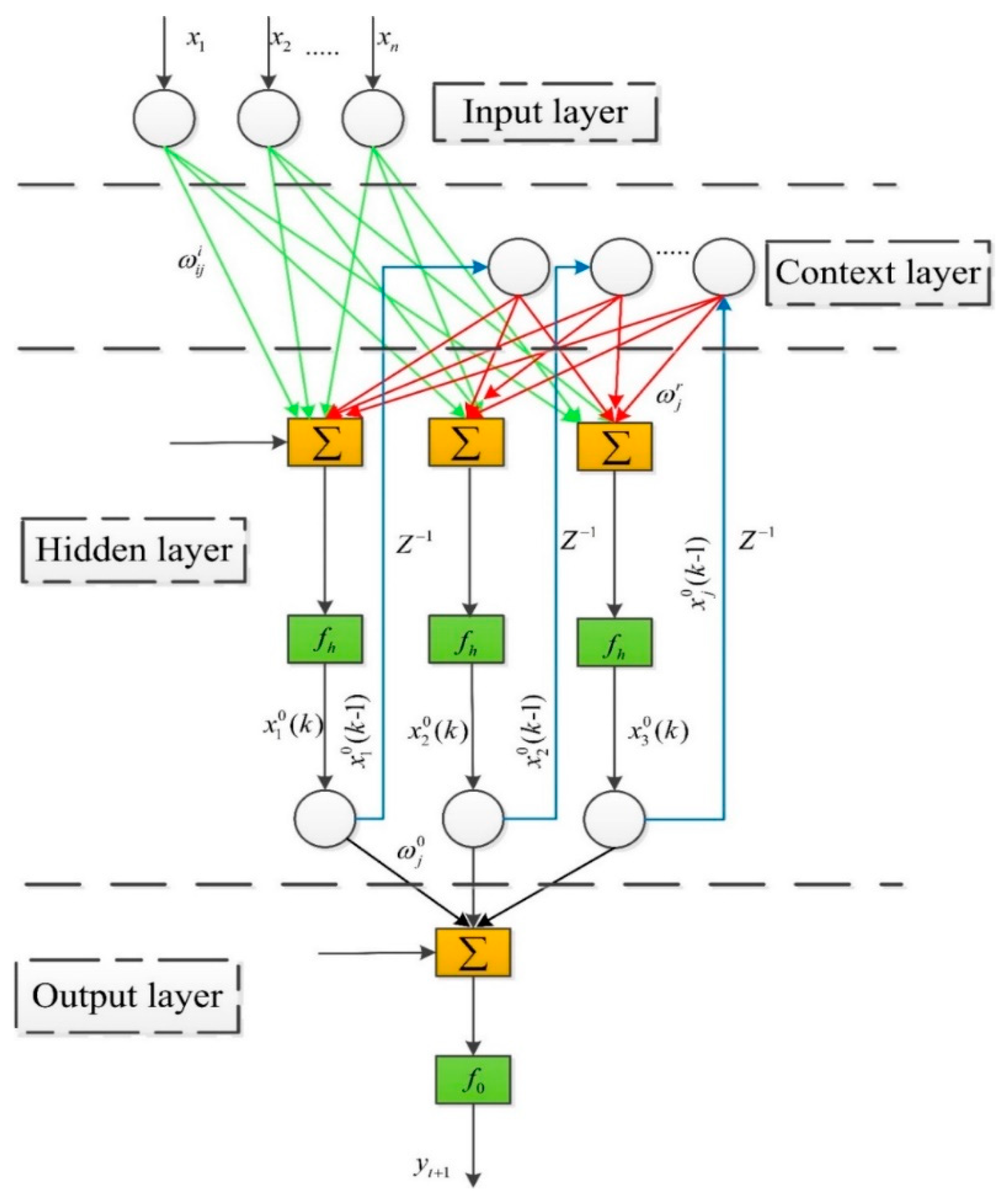
2.6. Elman Neural Network
2.7. Performance Evaluation Criteria
3. Empirical Study
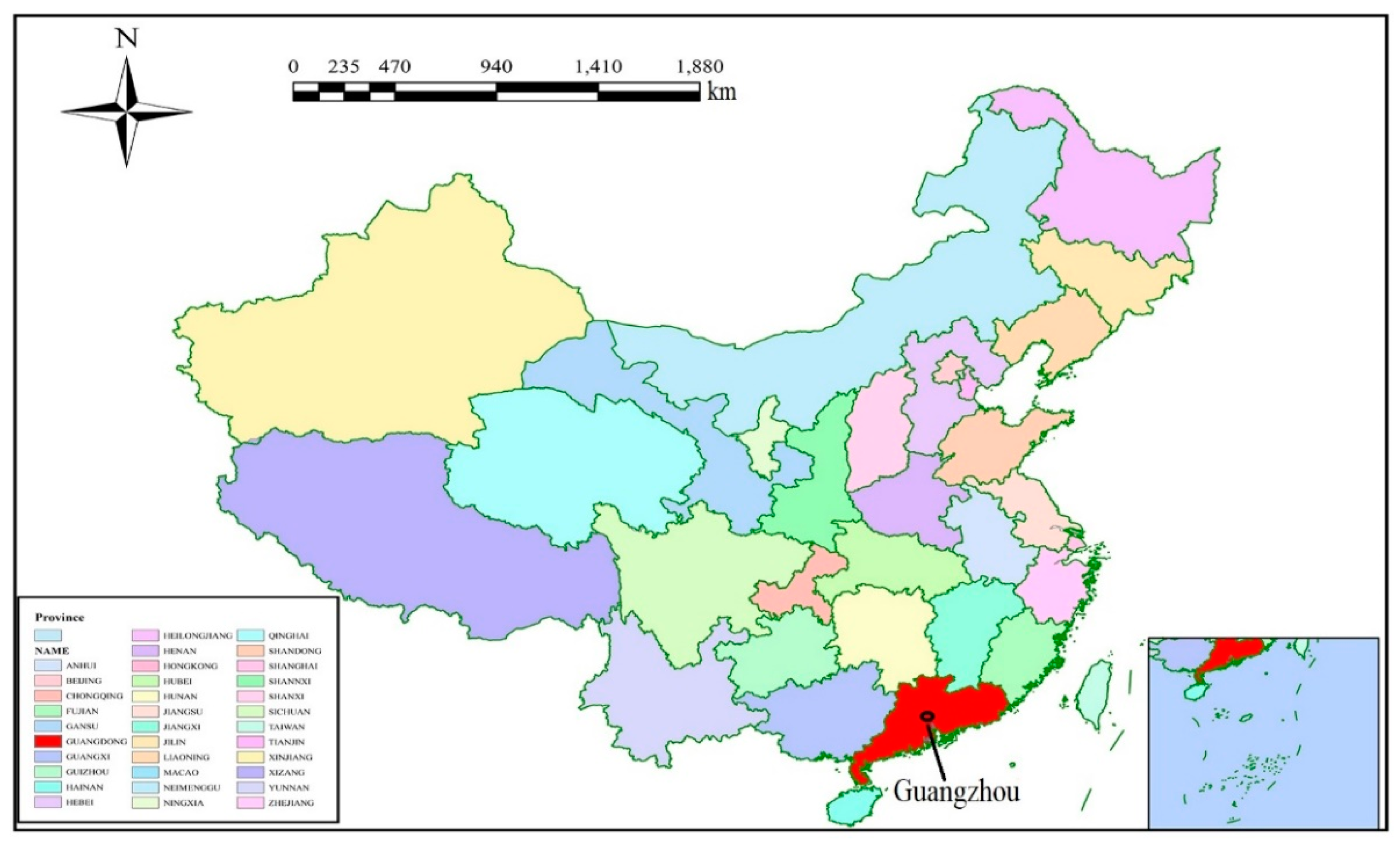
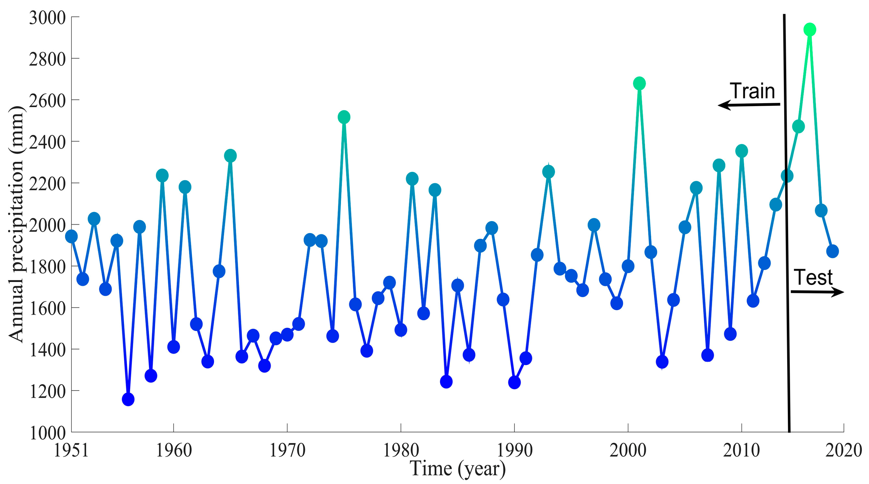
3.1. Study Area and Data Description
3.2. Model Forecasting Results
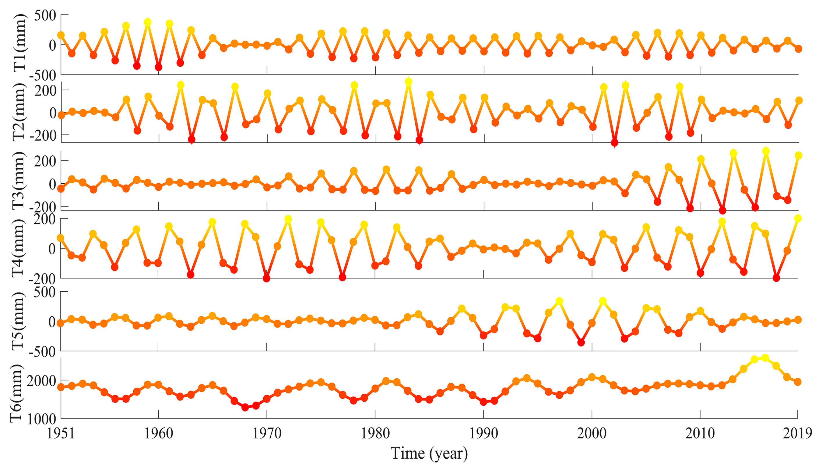
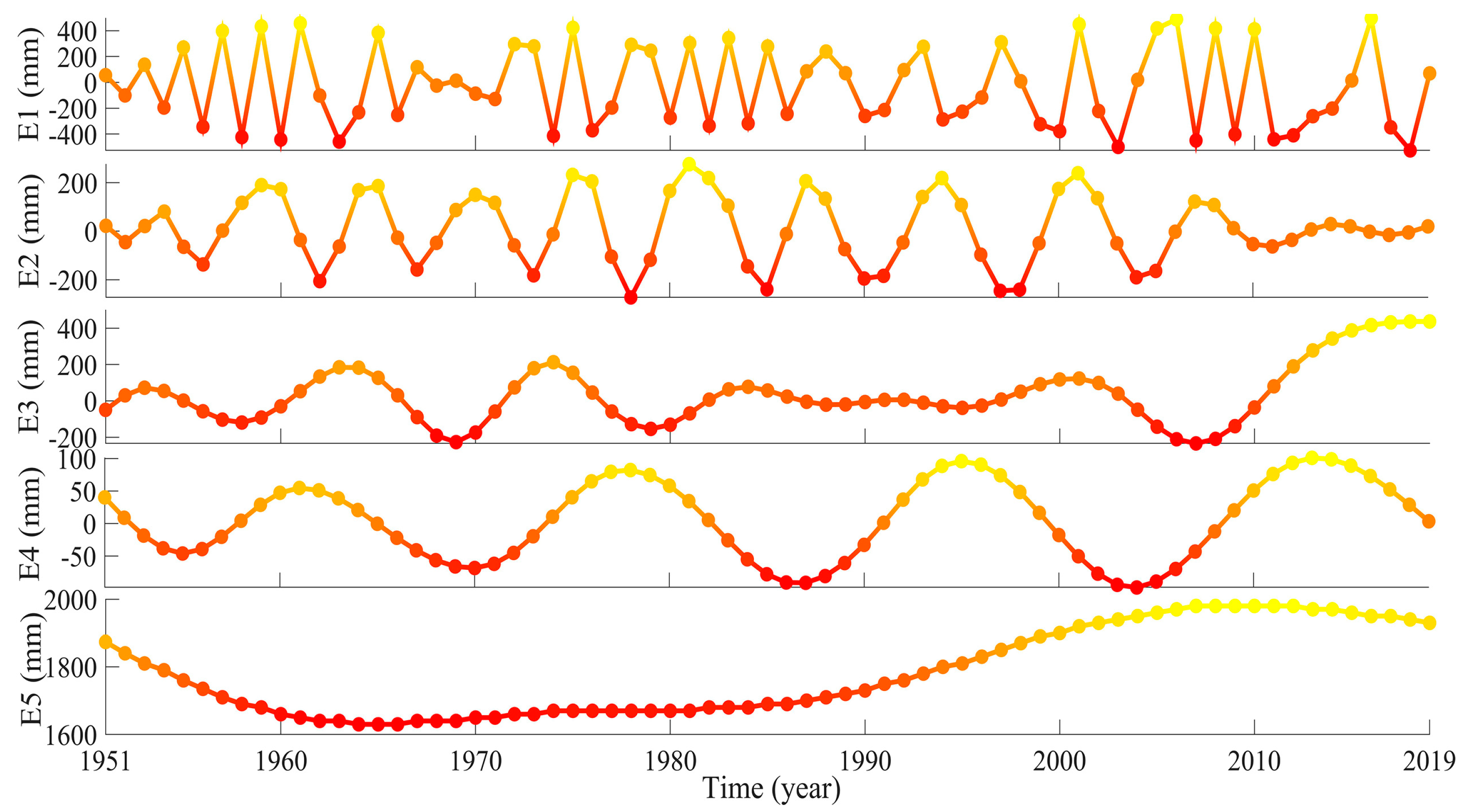
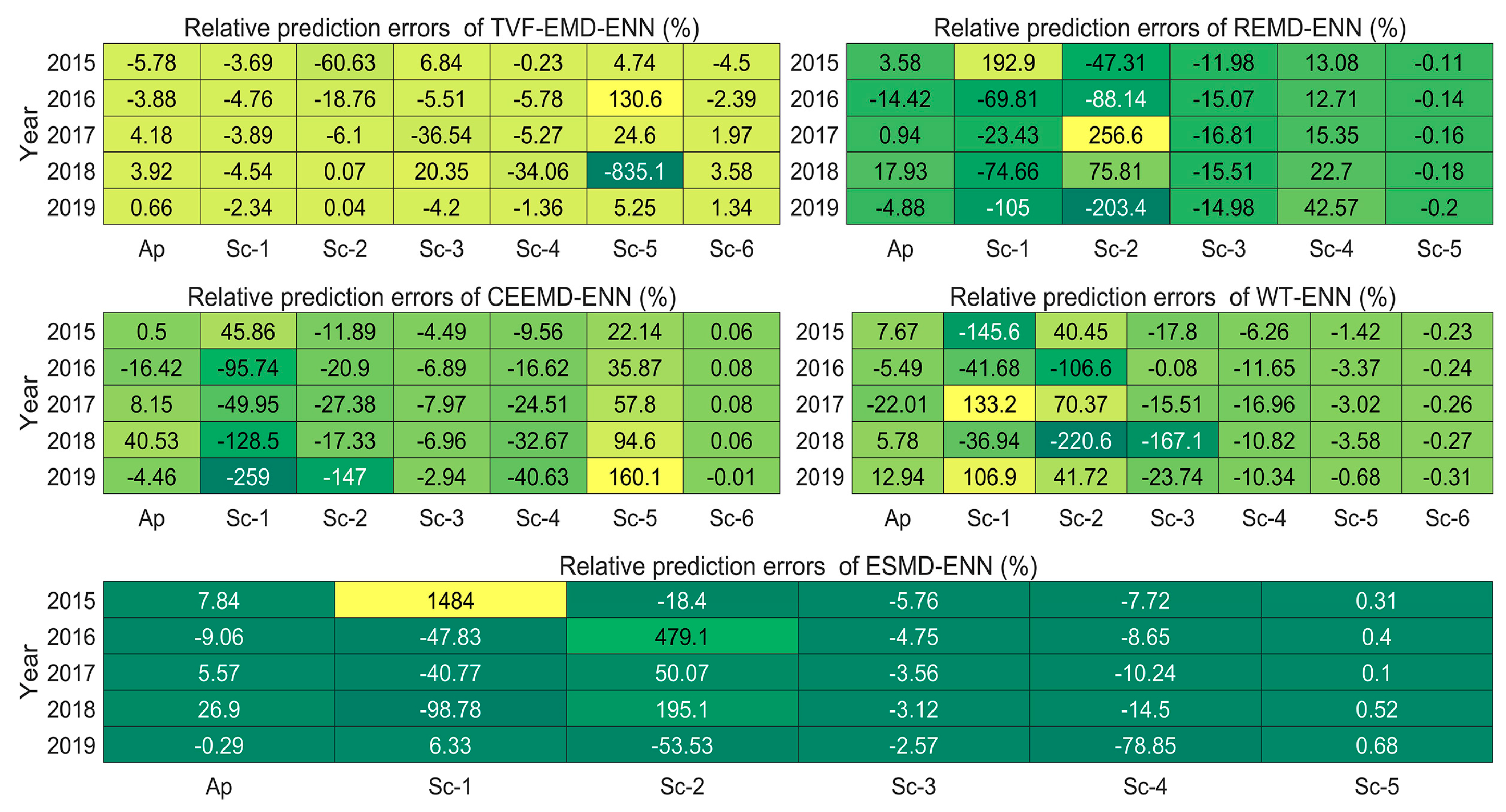
3.2.1. TVF-EMD-ENN Forecasting Results
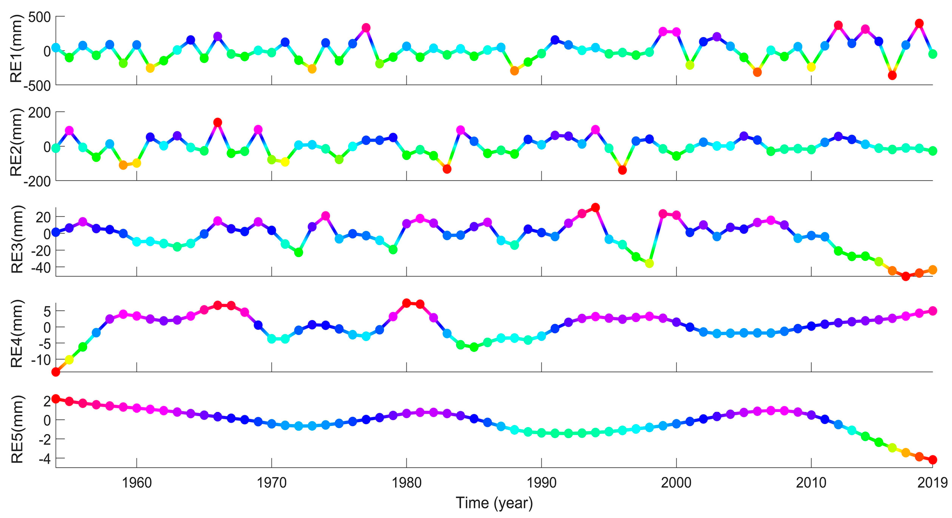
3.2.2. REMD-ENN Forecasting Results
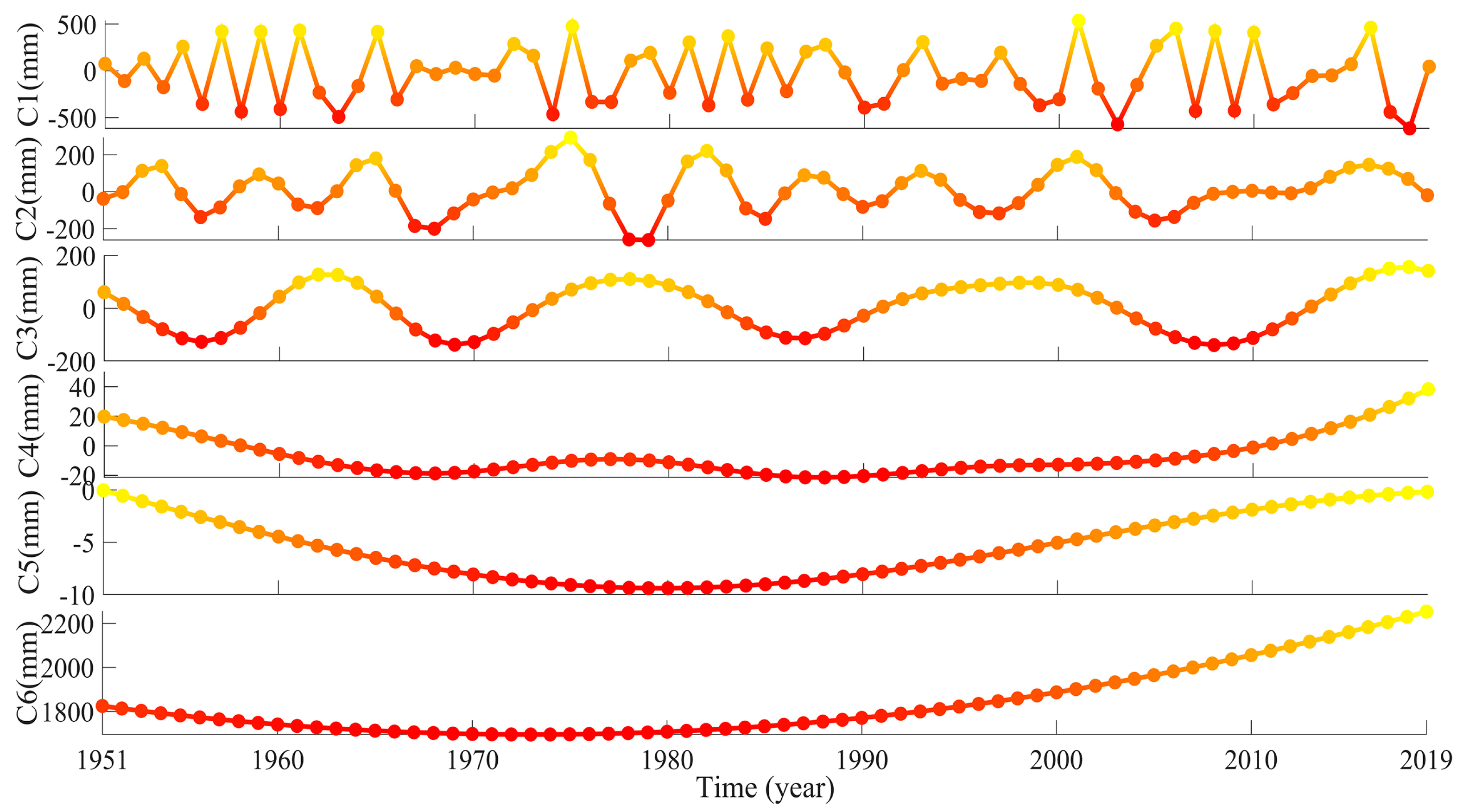
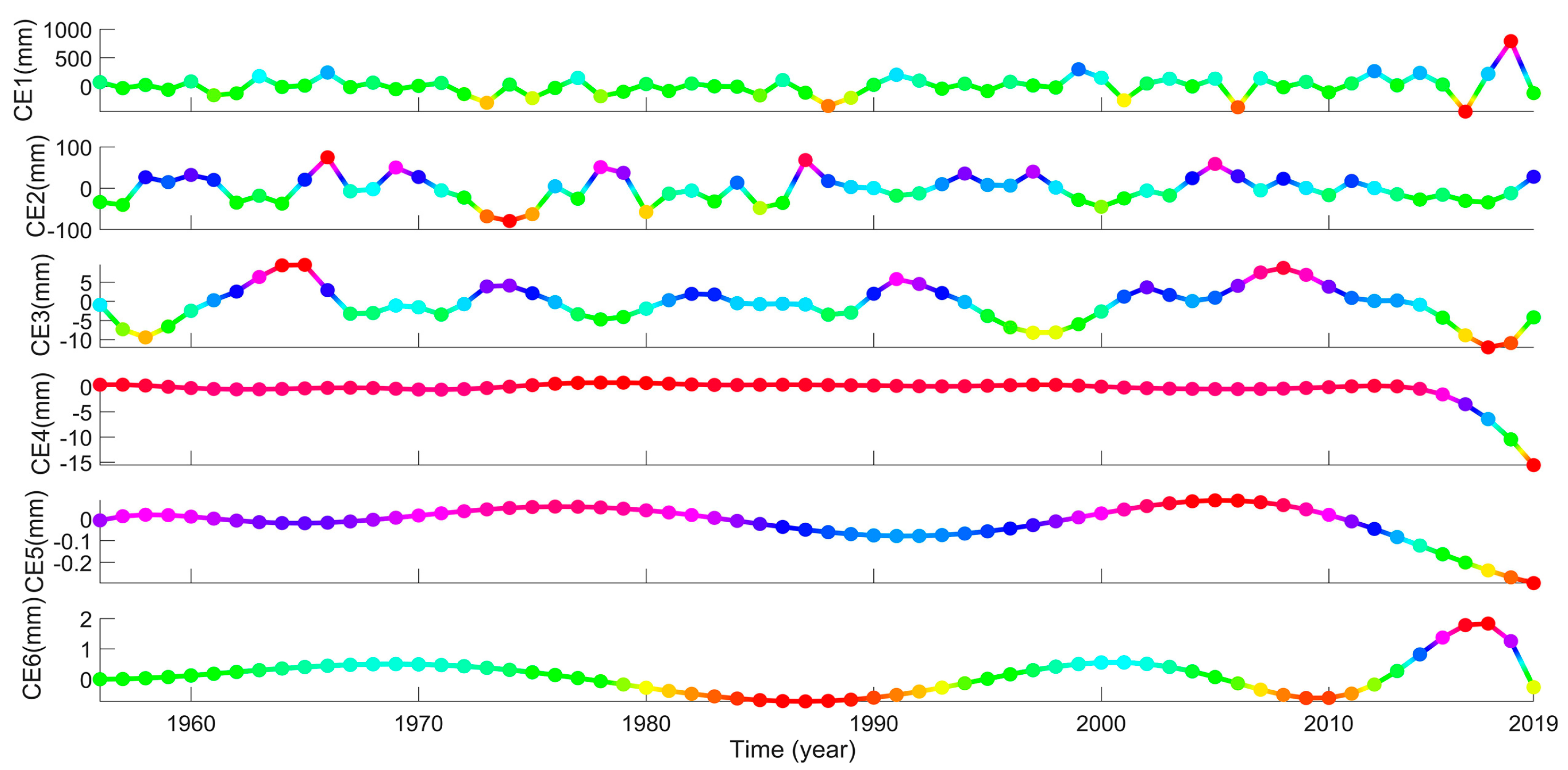
3.2.3. CEEMD-ENN Forecasting Results
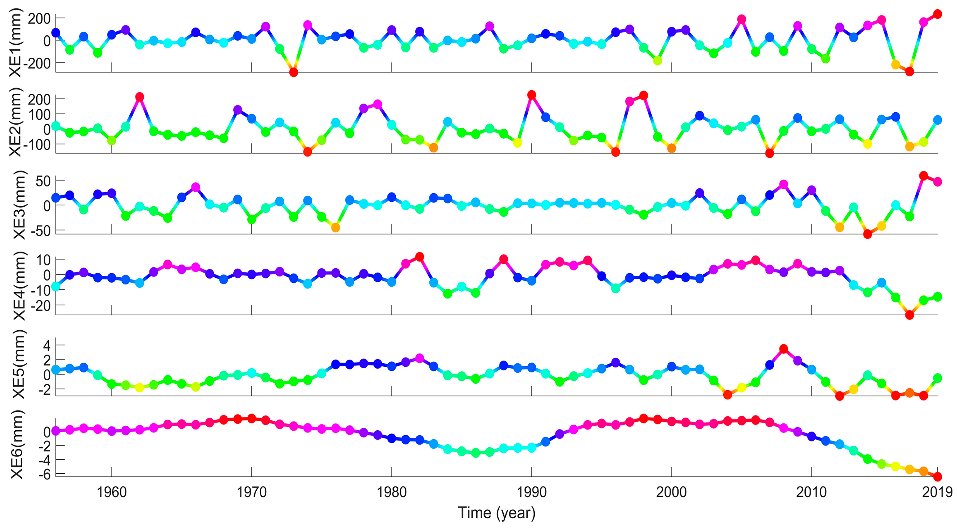
3.2.4. WT-ENN Forecasting Results
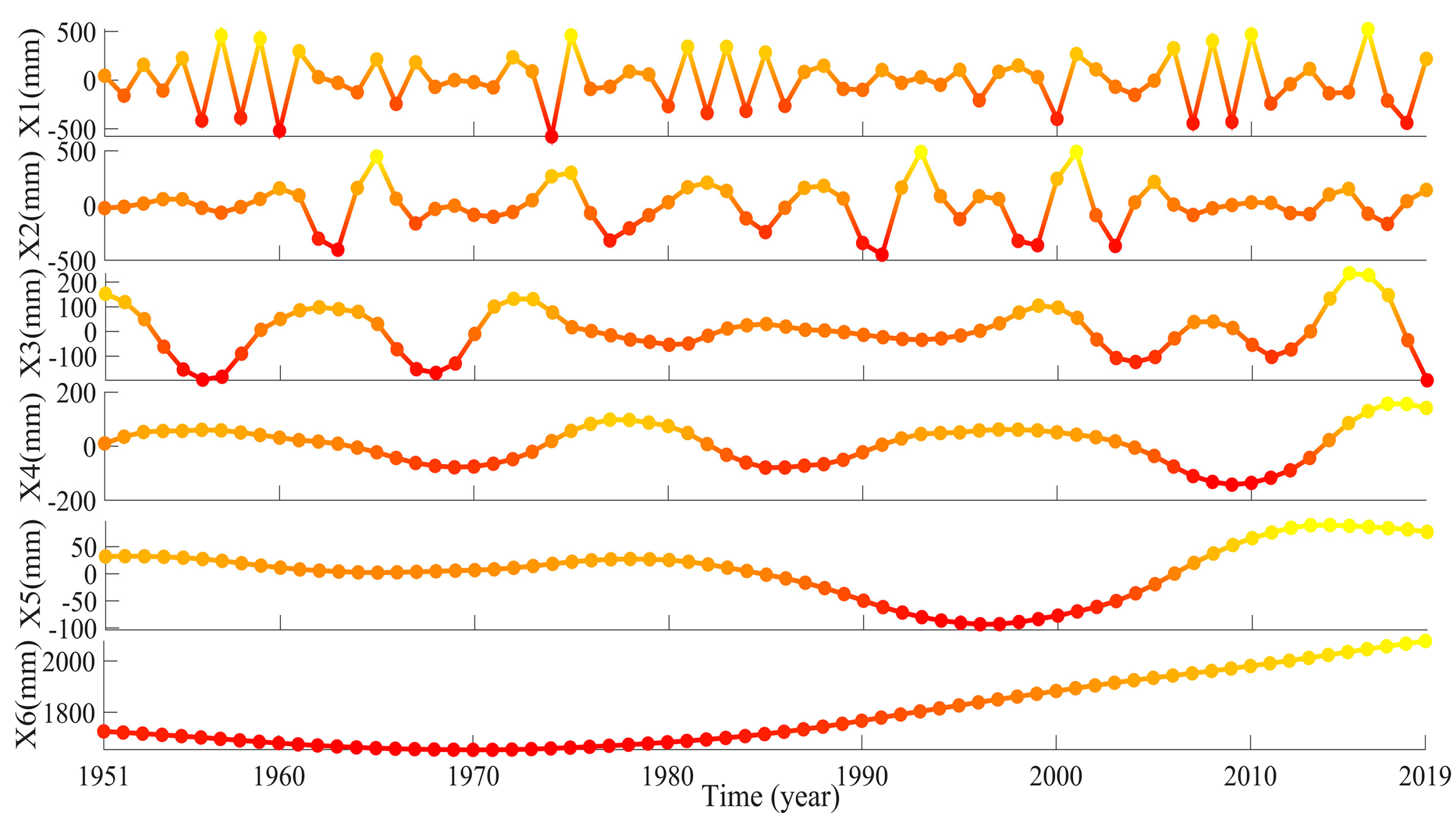
3.2.5. ESMD-ENN Forecasting Results
4. Results and Discussion
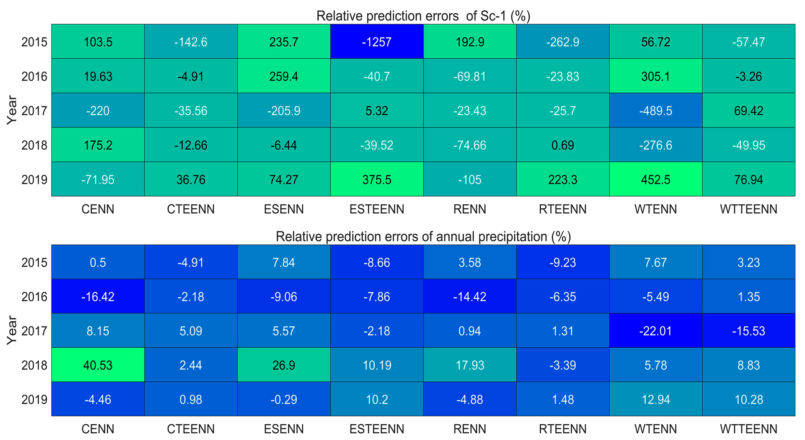
4.1. Reason for the Poor Prediction Performance of Sc-1
4.2. The Difference between the Five Decomposition Methods
4.3. Advantages of the Proposed Models over Traditional Machine Learning Models
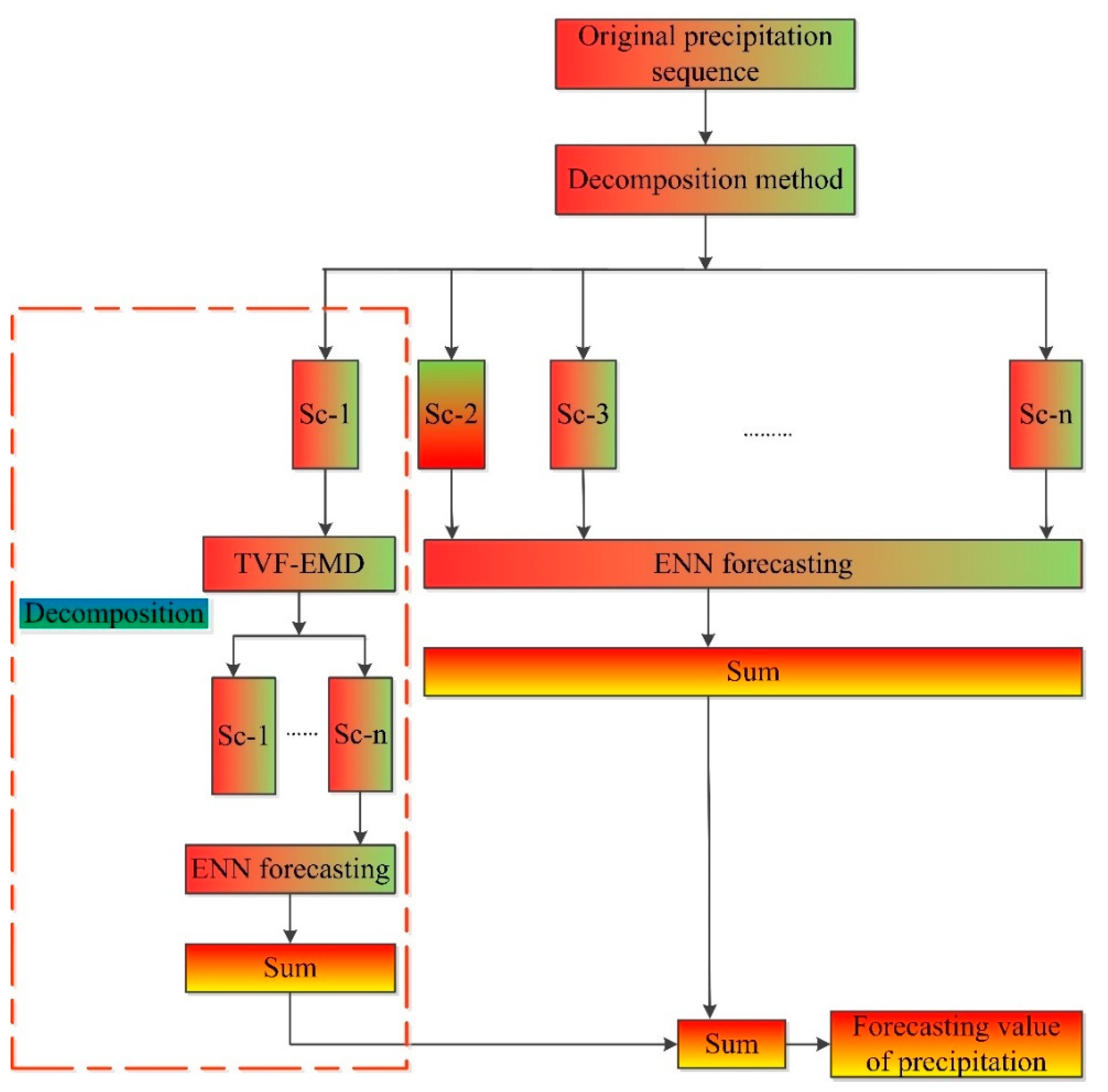
4.4. Improving the Prediction Performance of the Model
5. Conclusions
Author Contributions
Funding
Institutional Review Board Statement
Informed Consent Statement
Data Availability Statement
Conflicts of Interest
Acronyms
| TVF-EMD | Time-varying filter-based empirical mode decomposition |
| REMD | Robust empirical mode decomposition |
| CEEMD | Complementary ensemble empirical mode decomposition |
| ESMD | Extreme-point symmetric mode decomposition |
| WT | Wavelet transform |
| ENN | Elman neural network |
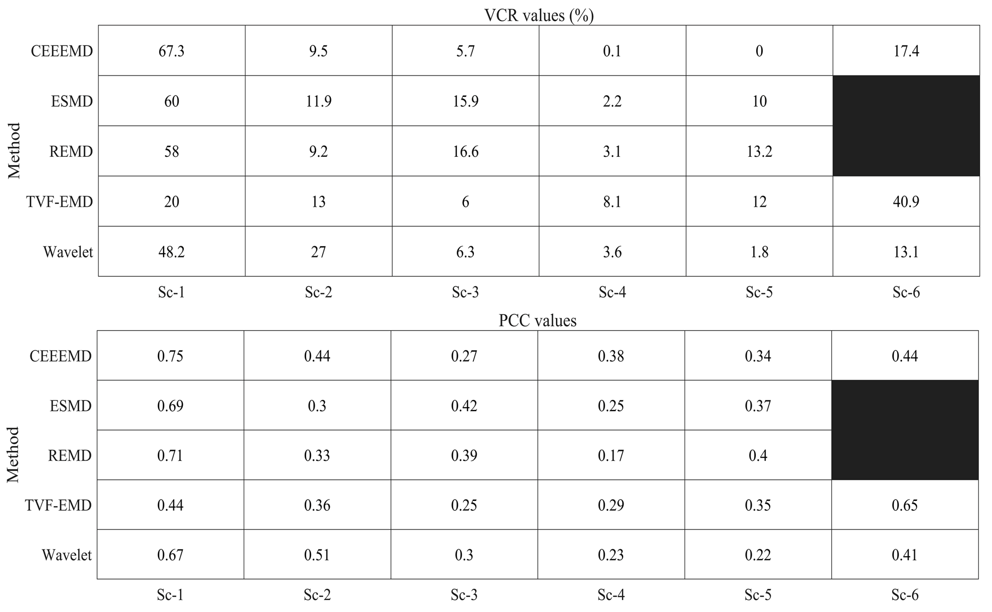
| VCR | Variance contribution rate |
| PCC | Pearson correlation coefficient |
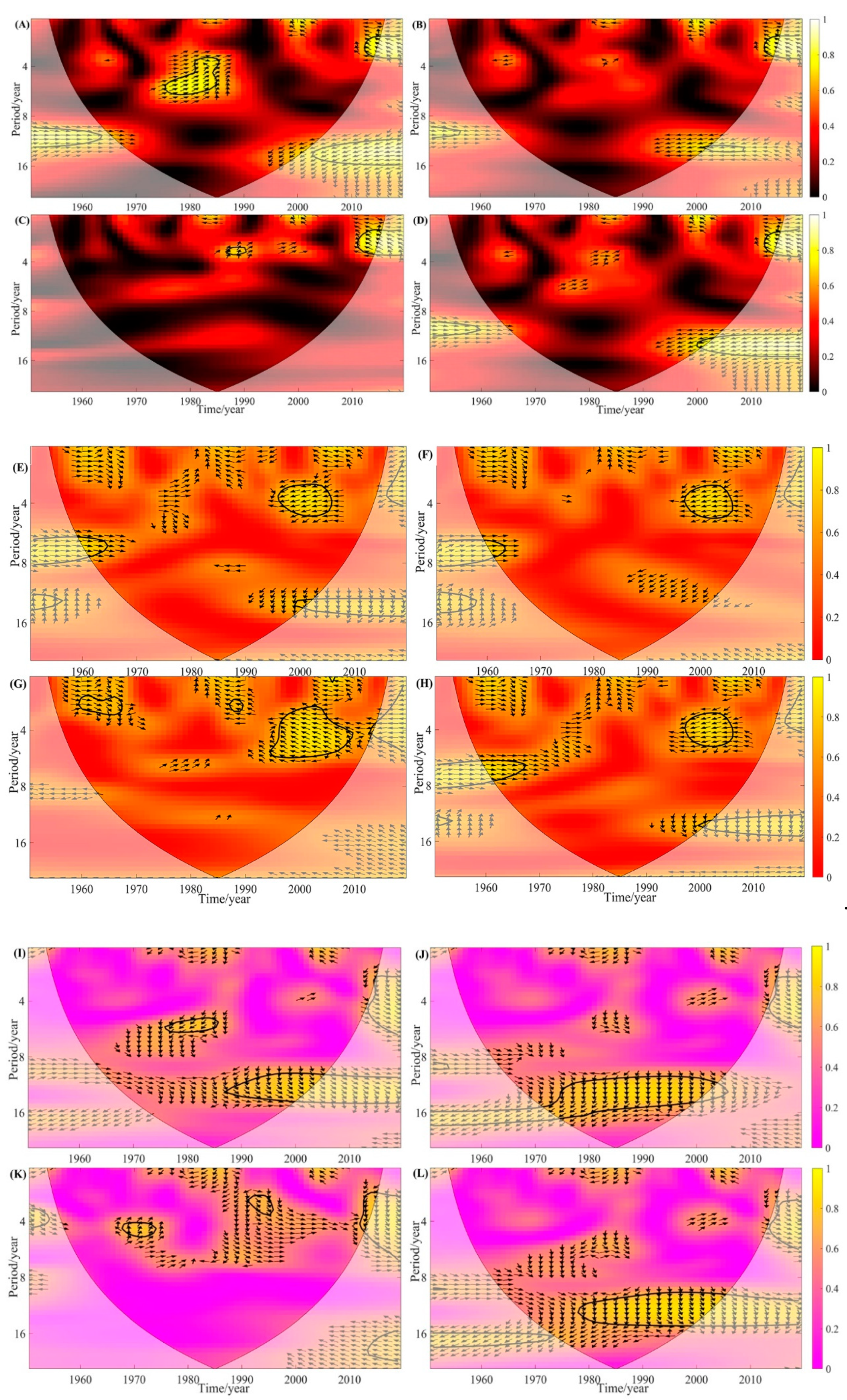
| WTC | Wavelet transform coherence |
| NAO | North Atlantic Oscillation |
| Sc-1 | The first subcomponent |
| RMSE | Root mean square error |
| MAE | Mean absolute error |
| MAPE | Mean absolute percentage error |
| R2 | Coefficient of determination |
| TVF-EMD-ENN | Time-varying filter-based empirical mode decomposition and Elman neural network |
| REMD-ENN | Robust empirical mode decomposition and Elman neural network |
| CEEMD-ENN | Complementary ensemble empirical mode decomposition and Elman neural network |
| ESMD-ENN | Extreme-point symmetric mode decomposition and Elman neural network |
| WT-ENN | Wavelet transform and Elman neural network |
| Tn | The Nth subcomponent obtained from TVF-EMD |
| TEn | The absolute prediction error of the Nth subcomponent obtained from TVF-EMD-ENN |
| Rn | The nth subcomponent obtained from REMD |
| REn | The absolute prediction error of the Nth subcomponent obtained from REMD-ENN |
| Cn | The nth subcomponent obtained from CEEMD |
| CEn | The absolute prediction error of the Nth subcomponent obtained from CEEMD-ENN |
| Xn | The nth subcomponent obtained from the WT |
| XEn | The absolute prediction error of the Nth subcomponent obtained from WT-ENN |
| EEn | The absolute prediction error of the Nth subcomponent obtained by ESMD-ENN |
| En | The nth subcomponent obtained from ESMD |
| COI | Cone of influence |
| CENN | CEEMD-ENN |
| CTEENN | CEEMD-TVF-EMD-ENN |
| ESENN | ESMD-ENN |
| ESTEENN | ESMD-TVF-EMD-ENN |
| RENN | REMD-ENN |
| RTEENN | REMD-TVF-EMD-ENN |
| WTENN | WT-ENN |
| WTTEENN | WT-TVF-EMD-ENN |
| LSTM | Long short-term memory neural network |
| RBF | Radial basis function neural network |
References
- Swain, S.; Patel, P.; Nandi, S. A multiple linear regression model for precipitation forecasting over Cuttack district, Odisha, India. In Proceedings of the 2nd International Conference for Convergence in Technology (I2CT), Mumbai, India, 1 April 2017; pp. 355–357. [Google Scholar] [CrossRef]
- Rahman, M.A.; Yunsheng, L.; Sultana, N. Analysis and prediction of rainfall trends over Bangladesh using Mann–Kendall, Spearman’s rho tests and ARIMA model. Meteorol. Atmos. Phys. 2017, 129, 409–424. [Google Scholar] [CrossRef]
- Amiri, S.S.; Mottahedi, M.; Asadi, S. Using multiple regression analysis to develop energy consumption indicators for commercial buildings in the US. Energy Build. 2015, 109, 209–216. [Google Scholar] [CrossRef]
- Ramirez, M.C.V.; De Campos Velho, H.F.; Ferreira, N.J. Artificial neural network technique for rainfall forecasting applied to the so Paulo region. J. Hydrol. 2005, 301, 146–162. [Google Scholar] [CrossRef]
- Ramana, R.V.; Krishna, B.; Kumar, S.R.; Pandey, N.G. Monthly Rainfall Prediction Using Wavelet Neural Network Analysis. Water Resour. Manag. 2013, 27, 3697–3711. [Google Scholar] [CrossRef]
- Mislan, M.; Haviluddin, H.; Hardwinarto, S.; Sumaryono, S.; Aipassa, M. Rainfall monthly prediction based on artificial neural network: A case study in Tenggarong station, east Kalimantan-Indonesia. Procedia Comput. Sci. 2015, 59, 142–151. [Google Scholar] [CrossRef]
- Wu, C.L.; Chau, K.W.; Fan, C. Prediction of rainfall time series using modular artificial neural networks coupled with data-preprocessing techniques. J. Hydrol. 2010, 389, 146–167. [Google Scholar] [CrossRef]
- Kim, T.; Heo, J.H.; Jeong, C.S. Multireservoir system optimization in the Han River basin using multi-objective genetic algorithms. Hydrol. Process. 2006, 20, 2057–2075. [Google Scholar] [CrossRef]
- Maryam, S.; Jan, A.; Ahmad, F.F.; Yagob, D.; Kazimierz, A. A wavelet-sarima-ann hybrid model for precipitation forecasting. J. Water Land Devt. 2016, 28, 27–36. [Google Scholar] [CrossRef]
- Chau, K.W.; Wu, C.L. A hybrid model coupled with singular spectrum analysis for daily rainfall prediction. J. Hydroinform. 2010, 12, 458–473. [Google Scholar] [CrossRef]
- Tan, Q.-F.; Lei, X.-H.; Wang, X.; Wang, H.; Wen, X.; Ji, Y.; Kang, A.-Q. An adaptive middle and long-term runoff forecast model using EEMD-ANN hybrid approach. J. Hydrol. 2018, 567, 767–780. [Google Scholar] [CrossRef]
- Chen, R.; Jia, H.; Xie, X.; Wen, G. Sparsity-Promoting Adaptive Coding with Robust Empirical Mode Decomposition for Image Restoration. In Pacific Rim Conference on Multimedia; Springer: Cham, Switzerland, 2017. [Google Scholar] [CrossRef]
- Mumtaz, A.; Ramendra, P.; Yong, X.; Zaher, M.Y. Complete ensemble empirical mode decomposition hybridized with random forest and kernel ridge regression model for monthly rainfall forecasts. J. Hydrol. 2020, 584, 124674. [Google Scholar] [CrossRef]
- Ji, Y.; Dong, H.T.; Xing, Z.X.; Sun, M.X.; Fu, Q.; Liu, D. Application of the decomposition prediction reconstruction framework to middle and long-term runoff forecasting. Water Supply. 2020. [Google Scholar] [CrossRef]
- Arab, A.M.; Amerian, Y.; Mesgari, M.S. Spatial and temporal monthly precipitation forecasting using wavelet transform and neural networks, Qara-Qum catchment. Iran. Arab. J. Geosci. 2016, 9, 1–18. [Google Scholar] [CrossRef]
- Partal, T.; Cigizoglu, H.K. Prediction of daily precipitation using wavelet—neural networks. Hydrol. Sci. J. 2009, 54, 234–246. [Google Scholar] [CrossRef]
- Qin, Y.H.; Li, B.F.; Sun, X.; Chen, Y.N.; Shi, X. Nonlinear response of runoff to atmospheric freezing level height variation based on hybrid prediction models. Hydrol. Sci. J. 2019, 64, 1556–1572. [Google Scholar] [CrossRef]
- Li, H.; Li, Z.; Mo, W. A time varying filter approach for empirical mode decomposition. Signal Process. 2017, 138, 146–158. [Google Scholar] [CrossRef]
- Zhang, X.; Liu, Z.; Miao, Q.; Wang, L. An optimized time varying filtering based empirical mode decomposition method with grey wolf optimizer for machinery fault diagnosis. J. Sound Vib. 2018, 418, 55–78. [Google Scholar] [CrossRef]
- Xu, Y.; Cai, Z.; Cai, X. An enhanced multipoint optimal minimum entropy deconvolution approach for bearing fault detection of spur gearbox. J. Mech. Sci. Technol. 2019, 33, 2573–2586. [Google Scholar] [CrossRef]
- Chen, P.C.; Wang, Y.H.; You, J.Y.; Wei, C.C. Comparison of methods for non-stationary hydrologic frequency analysis: Case study using annual maximum daily precipitation in Taiwan. J. Hydrol. 2017, 545, 197–211. [Google Scholar] [CrossRef]
- Yeh, J.R.; Shieh, J.S.; Huang, N.E. Complementary ensemble empirical mode decomposition: A novel noise enhanced data analysis method. Adv. Adapt. Data Anal. 2010, 2, 135–156. [Google Scholar] [CrossRef]
- Huang, N.E.; Shen, Z.; Long, S.R.; Wu, M.C.; Shih, H.H.; Zheng, Q.; Yen, N.-C.; Tung, C.C.; Liu, H.H. The empirical mode decomposition and the Hilbert spectrum for nonlinear and non-stationary time series analysis. Proc. R. Soc. A Math. Phys. Eng. Sci. 1998, 454, 903–995. [Google Scholar] [CrossRef]
- Nejad, H.F.; Nourani, V. Elevation of wavelet denoising performance via an ANN-based streamflow forecasting model. Int. J. Comput. Sci. Manag. Res. 2012, 1, 764–777. [Google Scholar]
- Adamowski, J.; Sun, K. Development of a coupled wavelet transform and neural network method for flow forecasting of non-perennial rivers in semi-arid watersheds. J. Hydrol. 2010, 390, 85–91. [Google Scholar] [CrossRef]
- Nourani, V.; Alami, M.T.; Aminfar, M.H. A combined neural-wavelet model for prediction of Ligvanchai watershed precipitation. Eng. Appl. Artif. Intell. 2009, 22, 466–472. [Google Scholar] [CrossRef]
- Benaouda, D.; Murtagh, F.; Starck, J.-L.; Renaud, O. Wavelet-based nonlinear multiScale decomposition model for electricity load forecasting. Neurocomputing 2006, 70, 139–154. [Google Scholar] [CrossRef]
- Wang, J.L.; Li, Z.J. Extreme-point symmetric mode decomposition method for data analysis. Adv. Adapt. Data Anal. 2013, 5, 1137. [Google Scholar] [CrossRef]
- Qin, Y.; Li, B.; Chen, Z.; Chen, Y.; Lian, L. Spatio-temporal variations of nonlinear trends of precipitation over an arid region of northwest China according to the extreme-point symmetric mode decomposition method. Int. J. Climatol. 2018, 38, 2239–2249. [Google Scholar] [CrossRef]
- Elman, J. Finding structure in time. Cogn. Sci. 1990, 14, 179–211. [Google Scholar] [CrossRef]
- Song, C.; Zhang, X.; Hu, D.; Tuo, W. Research on a coupling model for groundwater depth forecasting. Desalin. Water Treat. 2019, 142, 125–135. [Google Scholar] [CrossRef]
- Pan, Y.; Li, Y.; Ma, P.; Liang, D. New approach of friction model and identification for hydraulic system based on MAPSO-NMDS optimization Elman neural network. Adv. Mech. Eng. 2017, 9, 1–14. [Google Scholar] [CrossRef]
- Ardalani-Farsa, M.; Zolfaghari, S. Chaotic time series prediction with residual analysis method using hybrid Elman–NARX neural networks. Neurocomputing 2010, 73, 2540–2553. [Google Scholar] [CrossRef]
- Su, L.; Miao, C.; Duan, Q.; Lei, X.; Li, H. Multiple-wavelet coherence of world’s large rivers with meteorological factors and ocean signals. J. Geophys. Res. Atmos. 2019, 124, 4932–4954. [Google Scholar] [CrossRef]
- Grinsted, A.; Moore, J.C.; Jevrejeva, S. Application of the cross wavelet transform and wavelet coherence to geophysical time series. Nonlinear Process. Geophys. 2004, 11, 561–566. [Google Scholar] [CrossRef]


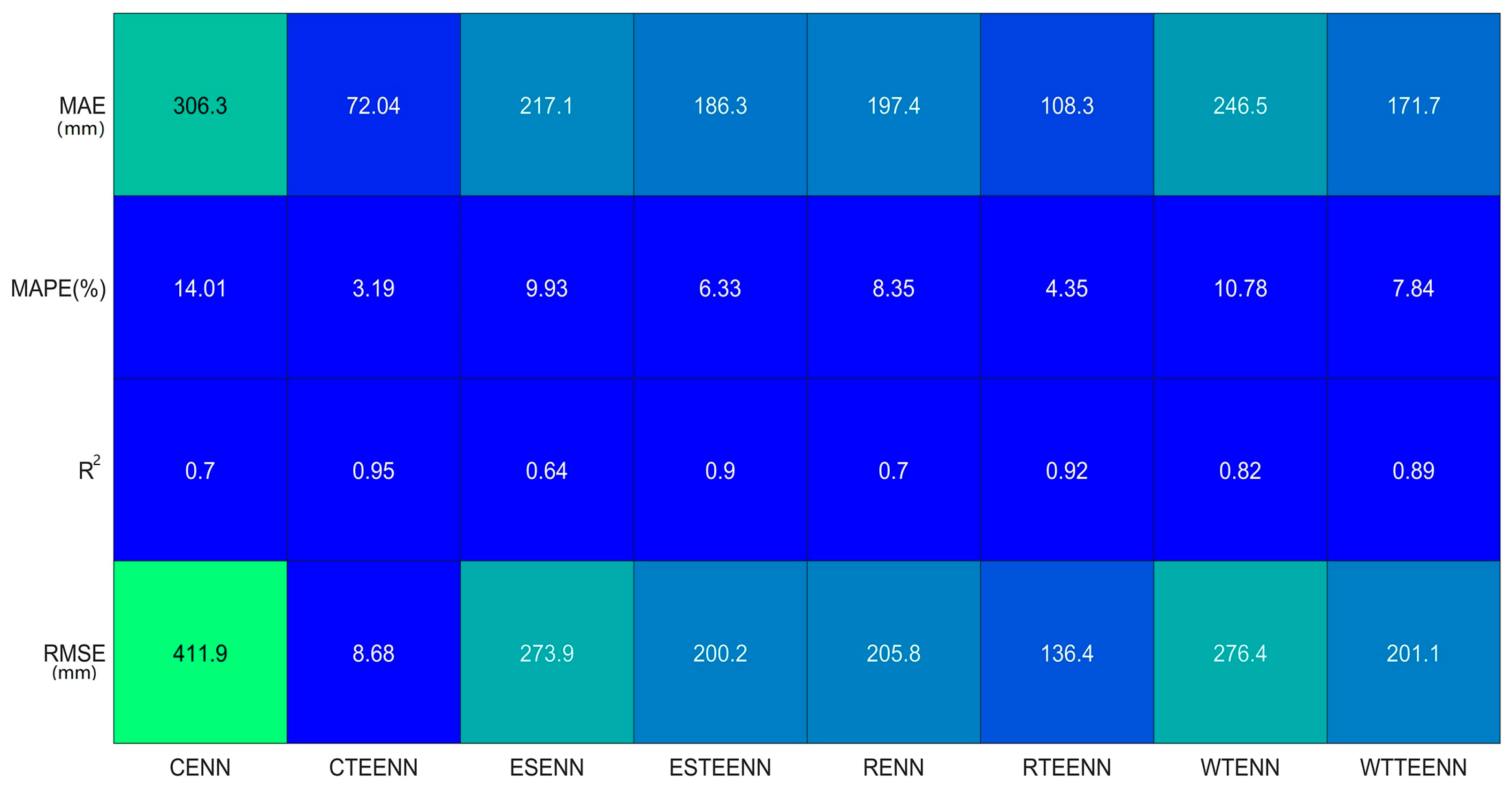
| Prediction Indices | Model | |||||||||
|---|---|---|---|---|---|---|---|---|---|---|
| CENN | EEENN | EENN | ENN | ESENN | LSTM | RBF | RENN | TEENN | WTENN | |
| MAE (mm) | 306.26 | 519.9 | 1076 | 1012 | 217.12 | 546.5 | 893.9 | 197.42 | 86.58 | 246.5 |
| MAPE (%) | 14.01 | 22.61 | 43.44 | 41.96 | 9.93 | 21.69 | 36.31 | 8.35 | 3.68 | 10.78 |
| R2 | 0.7 | 0.7 | 0.06 | 0.6 | 0.64 | 0.16 | 0.06 | 0.7 | 0.93 | 0.82 |
| RMSE (mm) | 411.89 | 581.6 | 1276 | 1120 | 273.88 | 631.4 | 967.1 | 250.85 | 96.48 | 276.42 |
Publisher’s Note: MDPI stays neutral with regard to jurisdictional claims in published maps and institutional affiliations. |
© 2021 by the authors. Licensee MDPI, Basel, Switzerland. This article is an open access article distributed under the terms and conditions of the Creative Commons Attribution (CC BY) license (http://creativecommons.org/licenses/by/4.0/).
Share and Cite
Song, C.; Chen, X. Performance Comparison of Machine Learning Models for Annual Precipitation Prediction Using Different Decomposition Methods. Remote Sens. 2021, 13, 1018. https://doi.org/10.3390/rs13051018
Song C, Chen X. Performance Comparison of Machine Learning Models for Annual Precipitation Prediction Using Different Decomposition Methods. Remote Sensing. 2021; 13(5):1018. https://doi.org/10.3390/rs13051018
Chicago/Turabian StyleSong, Chao, and Xiaohong Chen. 2021. "Performance Comparison of Machine Learning Models for Annual Precipitation Prediction Using Different Decomposition Methods" Remote Sensing 13, no. 5: 1018. https://doi.org/10.3390/rs13051018
APA StyleSong, C., & Chen, X. (2021). Performance Comparison of Machine Learning Models for Annual Precipitation Prediction Using Different Decomposition Methods. Remote Sensing, 13(5), 1018. https://doi.org/10.3390/rs13051018