Spatial and Multi-Temporal Analysis of Land Surface Temperature through Landsat 8 Images: Comparison of Algorithms in a Highly Polluted City (Granada)

Abstract

Over the past decade, satellite imaging has become a habitual way to determine the land surface temperature (LST). One means entails the use of Landsat 8 images, for which mono window (MW), single channel (SC) and split window (SW) algorithms are needed. Knowing the precision and seasonal variability of the LST can improve urban climate alteration studies, which ultimately help make sustainable decisions in terms of the greater resilience of cities. In this study we determine the LST of a mid-sized city, Granada (Spain), applying six Landsat 8 algorithms that are validated using ambient temperatures. In addition to having a unique geographical location, this city has high pollution and high daily temperature variations, so that it is a very appropriate site for study. Altogether, 11 images with very low cloudiness were taken into account, distributed between November 2019 and October 2020. After data validation by means of R² statistical analysis, the root mean square error (RMSE), mean bias error (MBE) and standard deviation (SD) were determined to obtain the coefficients of correlation. Panel data analysis is presented as a novel element with respect to the methods usually used. Results reveal that the SC algorithms prove more effective and reliable in determining the LST of the city studied here.

1. Introduction

The land surface temperature (LST) is an essential factor when studying physical processes on earth [1]. It is used for reference worldwide, in research dealing with local or regional space and in the fields of hydrology, meteorology, and superficial energy balance [2,3,4], as well as studies surrounding climatic change [5] and recent work involving the phenomenon known as urban heat island (UHI) [6,7,8,9,10]. It can be of vital importance to obtain a reliable LST, and this value could bear an impact upon the quality of life of populations. It has therefore become an essential factor, used to evaluate the interchange of water and superficial energy with the atmosphere [11].

Due to the important economic cost of measurements in situ and the difficulties involved in running them on vast extensions of territory, since the 1990s retrieval of remote sensing satellite images with sensors of thermal infrareds (TIRS) has become a more common approach. Training for the implementation of these systems is an important line of research [12] evidenced by the ample literature on the subject [12,13,14,15,16,17,18,19,20]. Still, the technological improvements incorporated by the infrared sensors of today’s satellites with respect to their predecessors urge researchers to keep on conducting research aimed at further advances in the field.

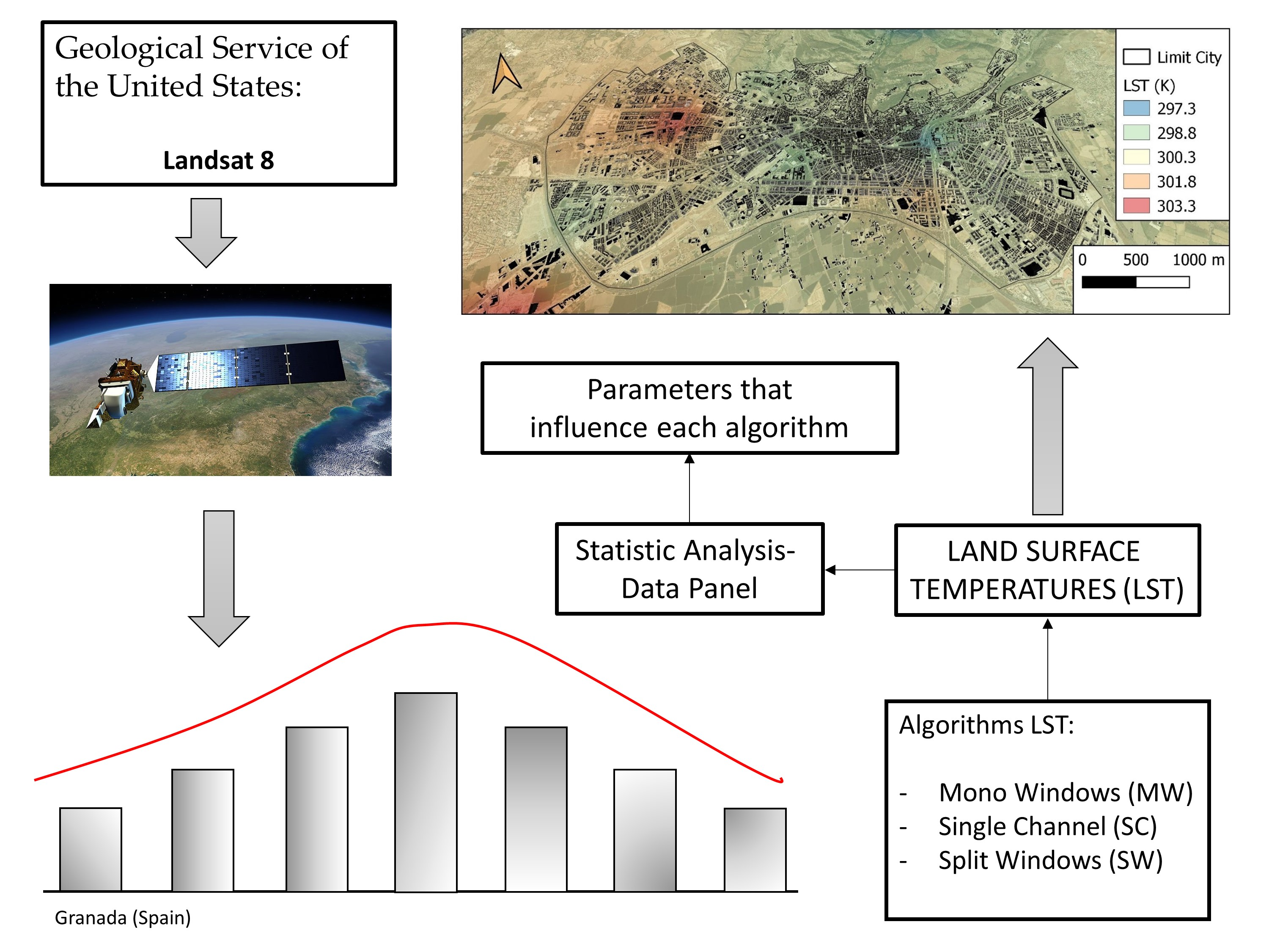
Numerous LST products have been developed based on satellite data. One of them, the Landsat, was the eighth satellite put into orbit in the year 2013. It features thermal infrared sensing (TIRS) bands 10 and 11, providing LST estimates of 16 days, and a 100-m resolution. When put into operation, the bands gave radiometric errors that surpassed the maximum value permitted (2%)—absolute values of 4%–5% were obtained for the measurements of band 10, and 8%–9% for band 11 [13]. To correct these deficiencies, authors Gerace and Montanaro (2017) [21] proposed an optical flare correction algorithm named the Stray Light Correction Algorithm (SLCA). It came into use in February 2017 for the images of the Terrestrial System of the US Geological Service (USGS) and is used for training in the field through a process of intervening validation [9,10,13,14,15].

Since the onset of its use, Landsat 8 has proved useful for determining the LST in large cities as well as prosperous, growing mid-size cities such as Lyon (France) [22], Krakow (Poland) [23] and Vienna (Austria) [24]. A variety of validated algorithms may be adopted to recover the LST through Landsat 8 satellite images [16,17,18,19,20,25,26]. They are based on the principles of fluid dynamics and atmospheric physics [27] and comprise three major groups: the mono window (MW) developed by Weng et al. (2004) and Qing et al. (2001) [17] and later improved by Wang et al. (2015) [28]; single channel (SC), developed by Jiménez and Sobrino et al. (2014) [16]; and, finally, the split window (SW) algorithms developed by Jimenez and Sobrino et al. (2014) [16], Du et al. (2015) [20] and Mao et al. (2005) [18]. The two first groups used a single TIRS channel for calculation, typically band 10; the latter group relied on two, bands 10 and 11. MW algorithms are based on individual atmospheric parameters: ambient temperature, humidity, and atmospheric mean temperature [12]. In turn, the SC algorithm [16] accounts for ground emissivity (ε) and steam-driven content of water (w) in the atmosphere (Yu et al. 2014). The great advantage of SW algorithms is that they do not require atmospheric data of great precision [29]. Thus, authors Jiménez et al. (2014) [16] established that they work well in global conditions and provide better results than SC algorithms. Xiangchen et al. (2019) [14] hold that SW algorithms are best suited for Landsat 8 estimates, though further investigation is necessary to validate the precision of these algorithms.

Currently, the use of algorithms to retrieve the LST presents two major challenges. 1. The spatial resolution of the pixels of LST systems can vary from 10⁻² to 10 Km² depending on the satellite used. This circumstance can give rise to pixels that represent various types of surfaces, which makes it difficult to obtain the LST [30]. 2. The satellite LST requires a verification process to validate the performance of the algorithms used. Common LST algorithm validation techniques are: in situ measurements, the radiance method, or cross reference and comparison with ambient temperatures near the ground. The first method is difficult and expensive, requiring radiometers located on terrains of homogeneous coverage (lakes, grasslands, dunes and regions with vegetation) and a dimension equal to the pixel of the satellite image. This method can give differences of 2 to 5 Kelvin degrees (K) with respect to actual measurements, according to previous studies [31]. For this reason, only a few validation studies using this method are found in the literature [32,33,34,35]. The main drawback of the second method is that it calls for knowing the emissivity of the soil and atmospheric profiles in situ. These can be simulated using MODTRAN 4.0 software, whose use is common in the literature [13,36,37] but requires verification that the simulated profiles are adapted to the actual atmosphere of the point studied [38]. The third method involves the validation of LST values retrieved against alternative LST values, either well documented or validated by other satellites [19,39]. It has the advantage of not requiring in situ or simulated measurements, but the precision is very sensitive to spatial and temporal mismatches of the measurements [30], and similar spatial resolutions are needed to proceed with the validation. In recent decades, the method of comparison with ambient temperatures near the ground (1–2 m) has gained importance as a validation system for LST algorithms [40,41,42,43,44]. It consists of comparing the recovered LST with the ambient temperature obtained from meteorological stations or temperature probes located near the ground. It is a fast, simple and low-cost method, but its main drawback lies in finding pure pixels of vegetation within cities that do not comprise several surfaces [30,37]. This inconvenience is minimized by using Landsat 8, since the resolution of its thermal bands is 100 m—an adequate distance to locate green or bare areas within or adjacent to cities. The precision of this method has reported differences ranging from 0.2 to 7.8 K between the recovered LST and the measured ambient temperatures [40,41,42,43,44,45].

The city under study presents important problems related to the local climate, conditioned by its proximity to the Sierra Nevada mountain range (30 km away), with average heights of 2045 m above sea level, and to the Mediterranean coast (60 km away). Granada is located in a former basin of the Mediterranean Sea and is considered highly vulnerable to climate change, given its high rate of increasing temperature as compared to the rest of the planet [46,47]. In addition to these geographic and climatological elements, Granada faces environmental challenges, having become the third most polluted city in Spain [48]. To the best of our knowledge, ours is the first study dedicated to LST estimates using satellite images of this area, and one of the first conducted on a Spanish city, after research on Barcelona [49,50] and Madrid [51].

Numerous studies have come to positively link environmental pollution with an increase in LST in urban areas [30,52,53,54]. Paradoxically, although many LST studies involving Landsat 8 images have been validated by the method of comparison with ambient temperatures [40,41,42,43,44,45], the possible effect of contamination on the environment has not been assessed in terms of the precision and subsequent validation of the LST. In sum, the geographic, climatic and high pollution conditions of the city of Granada make it an ideal place for this research.

The main statistical approaches and methods commonly used in studies of LST recovered through Landsat 8 images are: descriptive statistics of linear correlations and regressions [35,55,56,57], multiple regression analysis (MRA) [58,59], bivariate correlation [60] and ANOVA [61,62,63]. The panel data method used in this research allows for the incorporation of a greater number of data and variables, admitting the inclusion of individual effects of a certain variable to derive global results. It also allows inclusion of the spatial residual values of the results and eliminates the usual problem of collinearity between variables. Such considerations are often neglected by traditional methods, impeding the arrival at more accurate and complete results.

Therefore, the questions that we aim to answer through this research, in view of the particular characteristics of the city of Granada, are the following: (1) How does one choose the right LST algorithm for Landsat 8? (2) Is the validation method of comparison with ambient temperatures adequate? (3) Does panel data statistical analysis lead to different data than traditional analysis methods?

The foremost objective of this research is to determine the precision and maturity of six LST algorithms on Landsat 8 images validated using the technique of comparing ambient temperatures over the city of Granada (Spain), with its unique geographic, environmental and pollution characteristics. Specific goals include: 1. Determining if high contamination can affect the validation process of the chosen LST. 2. Providing a new low-cost, fast and accurate approach that allows the variations of the LST of cities to be monitored in an urgent and precise way, taking into account physical, environmental and climatic variables. In the long term, such efforts may contribute to decision-making by urban planners and public administrations about the distribution of the LST inside cities.

2. Materials and Methods

2.1. Area of Study and Data Source

The area studied is the city of Granada, in southern Spain. The geographic coordinates (UTM) of the metropolis are: latitude 37.111741° N and longitude 03.362401° W, and its altitude is 680 m above sea level (Figure 1). The local weather is strongly conditioned by its location at the feet of the Sierra Nevada, a major Andalusian mountain range with an average height of 2045 m a.s.l. After the Alps, it is the highest range in western Europe, The peak of Mulhacén is 3482 m a.s.l. According to the Koppen Geiger climatic classification, it features transitional weather between the Mediterranean climate (Bsk) and a cold semiarid climate of moist, mild winters and warm, dry summers [64]. The average yearly temperature fluctuates between 279.65 K in January and 298.45 K in the month of July, with a winter average of 270.15 K and summertime extremes of 316.15 K. The number of hours of sunshine per year is 2917 h, giving a mean of 7.99 h of sun a day. The population is 232,462, although it reaches 540,000 with the inclusion of Granada’s metropolitan area, which occupies a total surface of 880,000 km².

2.2. Landsat 8 Images

The satellite Landsat 8 was put into orbit in February 2013 and features two novel sweeping instruments: thermal infrared sensing (TIRS) and the Operational Land Imager (OLI). Images consist of eight spectral bands with 30 m resolution (bands 1 to 7 and 9), one band with 15 m resolution (band 8) and two thermal bands that allow for determining the LST (bands 10 and 11) with a resolution of 100 m [6,10]. These two TIRS bands work with a wavelength interval from 10.6 to 11.19 µm (band 10) and from 11.50 to 12.51 µm (band 11).

The city of Granada lies under the path of satellite Landsat 8, road 20, route 34. The images selected for this study are temporally located between November 2018 and October 2019. In the course of this span, 11 images with an index of cloudiness below 15 were used to enhance accuracy in obtaining the LST object. The images, indexed in

Table 1. Landsat 8 images used and acquired from the US Geological Service (USGS).

Number	Date (yymmdd)	UTC Time (hhmm)	Cloudiness (%)	Name File Landsat 8	L↑λ (Wm-2 sr-1μm-1)	L↓λ (Wm-2 sr-1μm-1)	Ꞇ	θsz (°)	V (m/s)
1	20191129	10:49	5	LC08_L1TP_20191129	0.45	0.75	0.77	63.08	0.83
2	20191215	10:49	1	LC08_L1TP_20191215	0.42	0.68	0.70	52.48	0.90
3	20191231	10:55	5	LC08_L1TP_20191231	0.49	0.80	0.82	45.00	1.10
4	20200217	10:49	11	LC08_L1TP_20200217	1.17	1.47	0.90	47.32	2.05
5	20200321	10:55	6	LC08_L1TP_20200321	1.88	2.10	0.67	61.18	1.94
6	20200625	10:49	0	LC08_L1TP_20200625	2.10	2.50	0.90	55.40	1.16
7	20200711	10:50	1	LC08_L1TP_20200711	2.24	2.65	0.85	51.24	1.23
8	20200727	10:50	13	LC08_L1TP_20200727	2.34	3.06	0.80	61.34	1.09
9	20200828	10:50	5	LC08_L1TP_20200828	2.12	2.65	0.79	62.04	2.01
10	20200929	10:50	3	LC08_L1TP_20200929	1.40	1.80	0.81	61.80	1.95
11	20201015	10:50	1	LC08_L1TP_20201015	1.12	1.40	0.92	53.25	2.33

, were acquired from the Geological Service of the United States (USGS). Meteorological conditions (solar radiation, wind, precipitation, etc.) can alter the measurements of the satellite spectrometer. The days selected for obtaining the images did not present precipitation in the previous 96 h, and the wind speed remained at constant values between 0.83 m/s and 2.22 m/s. The atmospheric parameters (L ^↑ _λ, L _{↓ λ} and wind speed) were obtained from Spain’s National Meteorological Agency (AEMET). The solar zenith angle θse was obtained from Landsat metadata files and the θsz values are equal to θse−90°.

After downloading the images, the spatial resolutions of bands 10 and 11 were reclassified to a resolution of 30 m, equal to the resolution of the rest of the Landsat 8 bands. This process was carried out using the raster calculator option of QGIS software, version 3.10.5, providing homogeneous and compatible pixels for the LST and emissivity. The processed images were georeferenced using the projection system ETRS89/UTM Zone 30N. Performing atmospheric correction in bands OLI entailed use of the algorithm Dark Object Subtraction (DOS) [12] by means of the Classification Plugin (SCP) with open source software QGIS [10,63,64,65,66,67,68].

2.3. Measurements of Ambient Temperatures

Spain’s National Meteorological Agency (AEMET) has two meteorology stations in Granada with instrumentation for measuring environmental parameters, calibrated according to international standards. The first is located in a rural area 12 km from the city (UTM: 37.11.45 N; 3.47.22 W), while the second is within the city (UTM: 37.11.23 N; 3.35.44 W). In order to minimize the impact that the urban environment and pollution conditions can have on the stations, we decided not to take into account the data of the second. The station used for reference, then, is found in an area of bare soil having a sufficient surface area for the Landsat 8-pixel (100 × 100 m) to allow for uniform and homogeneous results.

To ensure a greater number of environmental temperature comparison points, five certified temperature and humidity monitoring elements (Testo brand, model 184H) with calibration certificates were placed in a well-distributed manner throughout the city. In choosing the location of the measurement points, two criteria were established: (1) Aspire to an equitable distribution of probes in urban, suburban, green and rural areas. (2) Have consent from Granada’s City Council when the probes were situated on public urban furniture. Figure 1 and

Table 2. Position and characteristics of the sites where the monitoring points were located.

Site	Lat/Lon	Elevation (m)	Land Cover	Zone
Almunia Park	37.19 N/−3.62 W	656.73	Buildings	Periphery
Fuentenueva	37.18 N/−3.60 W	669.32	Green Space	Downtown
Albayzín	37.18 N/−3.59 W	698.44	Buildings	Downtown
Ronda road	37.17 N/−3.60 W	662.46	Buildings	Downtown
Zaidín	37.15 N/−3.38 W	691.53	Buildings	Periphery
Weather Station	37.16 N/−3.60 W	661.63	Farmland	Rural Zone

indicate the positions selected for these five monitoring trials. A sixth measurement device was placed next to the meteorological station so as to check for possible differences or errors in readings that could invalidate the results obtained. Before commissioning, all the probes were set to measure the environmental conditions of a single point for two days, giving no differences in the measurements obtained.

The dataloggers were programmed so that they reliably registered the temperature and humidity values every 15 min during the entire study period. A total of 175,200 data for humidity and another 175,200 for temperature were thus obtained. They presented temperatures that oscillated between 253.15 K and 343.15 K, with an accuracy of ±0.5 K (273.15–343.15 K) and of ±0.8 K (253.15–273.15 K) with ±0.1 K. With regard to humidity, accuracy was ±2% to 298.15 K (20% to 80% DH) and ±3% to 298.15 K (20% and 80% DH). The datalogger confirmed calibration.

2.4. Methodology

The methodology applied in this research is depicted in Figure 2.

After downloading the Landsat 8 images identified in Table 1, we processed and georeferenced them. Next, we derived the values of normalized vegetation index (NDVI), fractional vegetation cover (PV), top of atmosphere (TOA), at sensor temperature brightness (Tb) and soil emissivity required by the different algorithms (MW, CS, SW) to determine the LST. In order to validate the recovered LST values, we compared them with the ambient temperatures near the ground (1–2 m) obtained using temperature and humidity probes, and the correlation coefficients were calculated. Subsequently, and using the panel data technique, the relationships between the LST variable and the rest of the variables included in each algorithm were obtained in order to identify the variability of the data and their reliability. The use of this method in our research allowed us to reflect possible variations in the conditions of each variable contemplated in the final results pertaining to each algorithm, which makes it a powerful approach.

2.5. Determination of Soil Emissivity

LST recovery algorithms call for knowledge of the Earth’s surface emissivity (LSE). This can vary significantly depending on the vegetation, humidity, roughness and other soil parameters [12,30]. The method usually used in the literature to determine the LST together with the LSE is through the NDVI^THM calculation threshold [11,12,25,42,49,69]. Its use is considered suitable for the spectral ranges of 10 to 12 µm, among which lie the bands 10 and 11 of Landsat 8 [25]. This method was therefore selected for use in our study.

The Threshold of Calculation NDVI (NDVI^THM)

The normalized vegetation index (NDVI) is calculated by means of the spectral bands of the near-IR spectrum (band 5) and the red band (band 4). This index gives an estimate of the presence of vegetation in a zone. The NDVI values range between −1 and 1, the former indicating clear, depopulated grounds, the latter, dense vegetation. The calculation formula is as follows:

$$NDVI=\frac{{\rho }_5-{\rho }_4}{{\rho }_5+{\rho }_4},$$

(1)

where $\rho$₄ and $\rho$₅ are the values of band 4 of bands 4 and 5, respectively. With the results obtained from Equation (1), the fractional vegetation cover (PV) can be calculated. This index establishes the proportion of a covered area for the vegetation or soil type [70,71]. Equation (2), for the calculation of the PV, is derived from the NDVI [11]:

$$PV={\left[\frac{NDVI-NDV{I}_{min}}{NDV{I}_{max}-NDV{I}_{min}}\right]}^2,$$

(2)

where NDVI is the index of vegetation normalized by means of Formula (1); and NDVI max and NDVI min are the maximum and minimal values of the NDVI interval. With the data obtained through Formulas (1) and (2), the emissivity of the soil can be calculated using Formula (3) for band 10 and Formula (4) for band 11 [11,15] (

Table 3. Estimation of ground emissivity normalized vegetation index (NDVI^THM).

Bands	Ground Emissivity	NDVI
	0.973 − 0.0744$\rho 4$	NDVI < 0.2
10	εv + εs (1 − Pv) + Ci	0.2 ≤ NDVI ≤ 0.5	(3)
	εv + Ci	NDVI > 0.5
	εv= 0.9863; εs= 0.9668
	0.984 − 0.026$\rho$4	NDVI < 0.2
11	εv + εs (1 − Pv) + Ci	0.2 ≤ NDVI ≤ 0.5	(4)
	εv + Ci	NDVI > 0.5
	εv = 0.9896; εs = 0.9747

).

Here, εv and εs are emissivities of vegetation and ground, Ci is the coefficient of irregularity, and $\rho$4 is the value of band 4. The subindexes εv and εs indicated above correspond to Landsat 8 bands 10 and 11, respectively [11]. The Ci factor employed was Ci = 0 for flat surfaces [12].

2.6. Top of Atmosphere (TOA) and at Sensor Temperature Brightness (Tb)

The digital numbers (DNs) of the TIRS bands were converted into spectral radiance using the following equation [10,72]:

$$L\lambda =M_L \times Q_{Cal}+A_L$$

(5)

where $L\lambda$ is the spectral radiance at the top of the atmosphere (TOA) expressed in W/(m²∙sr∙μm); $M_L$ is the specific multiplying factor of the band located in the metadata index of the Landsat 8 images. For the TIRS bands, this factor is 3.342 × 10⁻⁴ W/(m²∙sr∙ μm); $Q_{Cal}$ is the digital variant value (DN) of the bands in the interval from 0 to 255, and $A_L$ is the additive factor of specific re-scaling of the TIRS bands, likewise included in the archives of meta-bits of information from the images.

From here on, the spectral radiance (L_λ) is converted and expressed as temperature brightness (Tb) in Kelvin. To this end, the conversion constants used are thermal K₁ and K₂ of the TIRS bands that appear in the file of metadata (band 10: K₁ 774.8553 and K₂ = 1321.0789; Band 11: K₁ = 480.8883 and K₂ = 120.1442). The formula used is [10,72]:

$$Tb=\frac{K_2}{\log \left(\frac{K_1}{L_{\lambda }}+1\right)} .$$

(6)

2.7. Description of the Algorithms of Temperature Recovery

2.7.1. Mono Window (MW) Algorithms

The first method used in the MW group to calculate the LST entails the validated algorithm [17]. The equation for its calculation is as follows:

$$LST=\frac{Tb}{\left(1+\left(\lambda \frac{Tb}{C_2}\right)x\log \left(\epsilon \right)\right)},$$

(7)

$$C_2=\frac{h x c}{s},$$

(8)

where LST is the land surface temperature, Tb is the temperature brightness of Landsat 8 TIRS 10, $\lambda$ is the wavelength of the emitted radiation (10.8 µm for band 10) and ε is ground emissivity. In Equation (8), C₂ = 1.4388 × 10⁻² m K, h is Planck’s constant of 6.626 × 10⁻³⁴ Js, c is the speed of light 2.998 × 10⁸ m/s, and s is the Boltzmann constant 1.38 × 10⁻²³ J/K [10,17].

The second method used involves the validated algorithm [19,28] calculated by:

$$LST=\frac{\left[a_{10}\left(1-C_{10}-D_{10}\right)+(b_{10}\left(1-C_{10}-D_{10}\right)+C_{10}-D_{10})T_{10}-D_{10}{T}_a\right]}{C_{10}},$$

(9)

$$C_{10}={\tau }_{10}{\epsilon }_{10},$$

(10)

$$D_{10}=\left(1-{\tau }_{10}\right)\left[1+\left(1-{\epsilon }_{10}\right){\tau }_{10}\right],$$

(11)

$$T_{a\left(Summer\right)}=16.0110+0.9262 T_o,$$

(12)

$$T_{a\left(Winter\right)}=19.2704+0.9112 T_o,$$

(13)

$${\tau }_{10\left(Summer\right)}=0.9184-0.0725 w,$$

(14)

$${\tau }_{10\left(Winter\right)}=0.9228-0.0735 w$$

(15)

where a₁₀ and b₁₀ are the counters used to approximate the derivative of Planck’s radiance function for TIRS band 10 with respective values of −62.7182 and 0.4339, T₁₀ is the Landsat 8 TIRS 10 temperature of brightness, Ꞇ₁₀ is the atmospheric transmittance of Landsat 8 TIRS band 10 for the periods of summer and winter, ε₁₀ is the ground emissivity for band 10, T_o is the air temperature close to the surface obtained with the datalogger, T_a is the effective atmospheric mean temperature in summer and winter, and $w$ is the total vapor content of the atmosphere [28,37].

2.7.2. Single Channel (SC) Algorithm

The method applied in the SC group to calculate the LST is the validated algorithm [16]. It is based on a polynomial approximation of the second order that depends on the content total of atmospheric vapor ($w$) expressed in a matrix notation by means of Equation (19). LST is estimated as:

$$\mathrm{LST}=\gamma \left[\frac{1}{\epsilon }\left({\psi }_1{L}_{TOA10}+{\psi }_2\right)+{\psi }_3\right]+\delta ,$$

(16)

$$\gamma =\frac{T{b}_{10}{}^2}{b_{\gamma }{L}_{TOA10}},$$

(17)

$$\delta =T_{b10}-\frac{T{b}_{10}{}^2}{b_{\gamma }},$$

(18)

$$\left[\begin{array}{c}{\psi }_1\\ {\psi }_2\\ {\psi }_3\end{array}\right]=\left[\begin{array}{ccc}0.04019& 0.02916& 1.01523\\ -0.38333& -1.50294& 0.20324\\ 0.00918& 1.36072& -0.27514\end{array}\right]x\left[\begin{array}{c}{w}^2\\ w\\ 1\end{array}\right]$$

(19)

where ε is the emissivity of the lot for band 10, L_{TOA 10} is the spectral radiance of band 10, b_γ is a constant value of 1324 for band 10, Tb₁₀ is the temperature of brightness of Landsat 8 TIRS band 10, and $w$ is the atmospheric vapor.

2.7.3. Split Window (SW) Algorithms

This type of TIR band algorithm refers to two channels, 10 and 11, and is based on the attenuation of radiance generated by the atmospheric absorption, established in two wavelengths between 10 and 12 µm. The first SW algorithm is validated [16] through the expression:

$$LST=T{b}_{10}+C_1\left(T{b}_{10}-T{b}_{11}\right)+C_2{\left(T{b}_{10}-T{b}_{11}\right)}^2+C_0+\left(C_3+C_{4}w\right)\left(1-\epsilon \right)+\left(C_5+C_{6}w\right)\Delta \epsilon$$

(20)

where Tb₁₀ and Tb₁₁ respectively represent the Landsat 8 TIRS temperature of brightness of bands 10 and 11, $w$ is the atmospheric vapor, ε and Δε are the values of the average emissivity and difference of emissivity between bands 10 and 11, respectively. The C coefficients used were: C₀ = −0.268, C₁ = 1.378, C₂ = 0.183, C₃ = 54.30, C₄ = −2.238, C₅ = −129.20 and C₆ = 16.40 [16] according to the steam-driven status of water in the atmosphere marked by the probes.

The second SW algorithm used in this study, validated after the previous one, was based on [20] and is expressed as:

$$\begin{array}{c}LST=b_0+\left(b_1+b_2\frac{1-\epsilon }{\epsilon }+b_3\frac{\Delta \epsilon }{{\epsilon }^2}\right)\frac{T{b}_{10}+T{b}_{11}}{2}\\ +\left(b_4+b_5\frac{1-\epsilon }{\epsilon }+b_6\frac{\Delta \epsilon }{{\epsilon }^2}\right)\frac{T{b}_{10}-T{b}_{11}}{2}\end{array}$$

(21)

where Tb₁₀ and Tb₁₁ respectively represent the Landsat 8 TIRS temperature of brightness of bands 10 and 11, ε and Δε are the values of the average emissivity and difference of emissivity between bands 10 and 11, respectively. The coefficients used were: b₀ = −2.78009, b₁ = 1.01408, b₂ = 0.15833, b₃ = −0.34991, b₄ = 4.04487, b₅ = 3.55414, b₆ = −8.88394 and b₇ = 0.9152, included in the status w of 0 and 2.5 gr cm⁻² [20].

The last SW algorithm used to calculate the LST was validated with new coefficients [18]. The expression for the calculation of the LST is as follows:

$$LST=T{b}_{10}+B_1\left(T{b}_{10}-T{b}_{11}\right)+B_0,$$

(22)

$$B_0=\frac{C_{11}\left(1-A_{10}-C_{10}\right)L_{10}-C_{10}\left(1-A_{11}-C_{11}\right)L_{11}}{C_{11}{A}_{10}-C_{10}{A}_{11}},$$

(23)

$$B_1=\frac{C_{10}}{C_{11}{A}_{10}-C_{10}{A}_{11}},$$

(24)

$$A_{10}={\epsilon }_{10}{\tau }_{10},$$

(25)

$$A_{11}={\epsilon }_{11}{\tau }_{11},$$

(26)

$$C_{10}=\left(1-{\tau }_{10}\right)\left(1+\left(1-{\epsilon }_{10}\right){\tau }_{10}\right),$$

(27)

$$C_{11}=\left(1-{\tau }_{11}\right)\left(1+\left(1-{\epsilon }_{11}\right){\tau }_{11}\right),$$

(28)

where Tb₁₀ and Tb₁₁ represent the temperature of brightness of Landsat 8 TIRS bands 10 and 11; ε₁₀ and ε₁₁ are the emissivity of the lot for bands 10 and 11. For the calculation of L₁₀ and L_11, the following expressions were used [15] for a temperature status between 293.15 and 323.15 K:

$$L_{10}=0.4464T_{b10}-66.61,$$

(29)

$$L_{11}=0.4831T_{b11}-71.23.$$

(30)

Calculating Ꞇ₁₀ and Ꞇ₁₁ (atmospheric transmittance for bands 10 and 11) entailed the simulation of local weather conditions, mainly with steam-driven water content [18,19]. We adopted the North American standard of 1976 and the MODTRAN summer atmospheric profile of mid-latitude, with a steam-driven status of water in the atmosphere between 0 and 3 gr cm⁻² [11]. Its expressions are:

$${\tau }_{10}=-0.0164w^2-0.04203w+0.9715,$$

(31)

$${\tau }_{11}=-0.0218w^2-0.07735w+0.9603,$$

(32)

where $w$ is the total vapor content of the atmosphere.

2.8. Identification of the Parameters for Each Algorithm

When calculating the LST, the algorithms (MW) must account for the parameters NDVI, VP, emissivity and temperature of brightness [17] and (SW) [16]. We added humidity to calculate the algorithms of the previous parameters (MW) [19,28], (SC) [16] and (SW) [18,20].

The reference serving to calculate air quality was the air pollution index (API), which is commonly used to measure air pollution [73,74,75,76]. Taking the form of a non-dimensional number in the range of 0 to 500, it provides a generalized degree of air pollution and the accompanying health hazards. Its statistical characteristics are described in

Table 4. Air pollution index (API) limit values.

API	Air Quality–Class	Air Quality–Evaluation	Health Effects
0–50	I	Excellent	Harmless
51–100	II	Good	Acceptable
101–200	III	Medium pollution	Sensitive
201–300	IV	Moderate pollution	Unhealthy
301–500	V	Severe pollution	Very unhealthy

.

The API is an integrated measure that reflects the levels of three fundamental air pollutants: SO₂, NO₂ and PM₁₀. Each is calculated individually, and the overall API of the city is derived from the highest API of these three air pollutants.

The interpolation to calculate the API of the city of Granada was performed using the following equation [74,76]:

$$API=\frac{\left(AP{I}_u-AP{I}_L\right)}{\left(C_u-C_l\right)\times \left(C_i-C_l\right)}+AP{I}_{Li},$$

(33)

where API is the index for pollutant i (the most substantial of the three pollutants SO₂, NO₂, and PM₁₀), C_i is the observed concentration of pollutant i, and C_u and C_l are the upper and lower limits of the range (shown in

Table 5. API concentration intervals.

API Intervals	SO2	NO2	PM10
0–50	0.000–0.050	0.000–0.080	0.000–0.050
51–100	0.050–0.150	0.080–0.120	0.050–0.150
101–200	0.150-0.800	0.120–0.280	0.150–0.350
201–300	0.800–1.600	0.280–0.565	0.350–0.420
301–500	1.600–2.620	0.565–0.940	0.0420–0.600

), within which the C_i, API_u and API_L are the upper and lower limits of the corresponding API interval (shown in Table 5). Finally, API_Li is the value of the lower range when moving to a higher range [74,76].

2.9. Strategy of Analysis

Data analysis was carried out using specialized statistical software, STATA, version 15. The first stage of analysis involved simple regression between the LST values obtained by means of the validated algorithms and the LST obtained in situ. Secondly, intervening analysis of the data set was performed using the panel data technique to appraise the statistical relation between the parameters of each algorithm employed.

The panel data technique for intervening statistical analysis is widely used in the literature and includes multi-changing models of relation [77,78,79]. This method allows for a greater number of data points in the analysis, which increases the degree of freedom while reducing the inconvenience of collinearity between the variables [80]. By taking into account individual effects, the final function obtained for the set of individuals is totally different from the one that would have been obtained using other statistical techniques [81]. It is mainly indicated for dealing with time series involving multiple individuals and quantitative variables, where the possibility exists that they change the explanatory variables in the relations between individuals [82]. Hence, this system of analysis was very well suited to the experimental data of our study.

Introducing this method of statistical analysis in our model entailed two phases [77]. In the first place, by means of the Hausman proof [80,81], the effects of the analysis are determined to be either fixed or random. Then, the model is estimated based on the results obtained in the tests of Wooldridge and Wald [80,81]. There are three methods of calculation: method of ordinary squares (MOS), generalized least squares (GLS) and method of intragroup estimators (MIE) [81].

The first of the three, while widely used for years, does not enable the effects of every individual to be analyzed over the course of time, which can give rise to biased estimators.

The second one is considered to be a more efficient extension than the first; it is assumed that the individual effects are not reflected in the explanatory variables of the model. In this case, the individual effects contribute to the error term, the expression of calculation being:

$$Y_{it}=\beta X_{it}+\left({\alpha }_i+{\mu }_{it}\right),$$

(34)

where ${\alpha }_i$ represents the individual effects, ${\mu }_{it}$ is the error of the model, β is coefficient and X are explanatory variables, i = individual and t = time.

The third method cited above assumes that the individual effects are in line with the explanatory variables, so that the individual effect is separated after error, the expression of calculation being as follows:

$$Y_{it}={\alpha }_i+\beta X_{it}+{\mu }_{it},$$

(35)

where, again, ${\alpha }_i$ are the individual effects, ${\mu }_{it}$ is the error of the model, β is coefficient and X are explanatory variables, i = individual and t = time.

3. Results

Before comparing the LST obtained by means of the different algorithms, we proceeded to compare the temperature and humidity data obtained from the AEMET meteorological station and the attached probe. The mean differences detected for temperature and relative humidity over the entire period were, respectively, ±0.1 K and ±1%. The readings of the temperature and humidity probes used in the city can thus be considered adequate for later use as a validation method supporting the results of this research.

3.1. General Comparison of LST Algorithms

The statistics obtained using the algorithms to calculate the LST are reflected in Figure 3. Overall, the algorithms presented higher annual mean values than the ones obtained with dataloggers, except for those reported by authors Wang et al. (2015) [28], which were lower but very close values.

The highest LST values were obtained with the group of SW algorithms, while the lowest values pertained to the group MW. The highest LST value of all (324.64 K) was obtained using the algorithm of authors Mao et al. (2005) [18]. To the contrary, the lowest value (276.27 K) was obtained by the method of Wang et al. (2015) [28]. This circumstance was similar for the case of mean temperatures, where the SW algorithms gave the highest mean LSTs, of values above 300 K, whereas the MW algorithms gave the lowest mean LSTs, under 296 K. The algorithm yielding the highest mean LSTs was that of authors Du et al. (2015) [20] (303.24 K), followed by that of Mao et al. (2005) [18], with an average LST just one-tenth less. The lowest mean LST was again obtained with the MW algorithm of authors Wang et al. (2015) [28] (292.31 K). By groups of algorithms, the SW gave a higher average value (302.56 K), the SC algorithm an intermediate value (299.49 K), and the MW the lowest average values (294.12 K). The median of all the algorithms seemed to be situated below the average, which implies a negative asymmetry of the LST obtained and a greater concentration of values in the third quartile. The variability of the data among quartiles 1–4 was in line with results of previous studies, excepting the one by Mao et al. (2005) [18], which presented a greater variability of data among the top 25%.

As seen in

Table 6. Comparison of LST estimates according to algorithm.

Group	Author	ΔT mean (K)	ΔT Mean Group (K)	SD (K)
MW	Qin et al. (2001) and Wang et al. (2015)	−6.90	−5.90	10.84
	Weng et al. (2004)	−4.90		10.39
SC	Jiménez et al. (2014)	0.28	0.28	11.82
	Jiménez et al. (2014)	1.73		12.64
SW	Du et al. (2015)	4.13	3.29	10.54
	Mao et al. (2005)	4.03		14.05

Note: ΔT: Mean temperature differences. SD: Standard deviation.

, a larger difference in means was obtained by Wang et al. (2015) [28], with a value of −6.90 K. The smallest difference corresponded to the SWA study by Jiménez et al. (2014) [16] with 0.28 K. As for the groups of algorithms, MW presented a difference of −5.40 K, algorithm SC an average difference of 0.28 K, and SW a difference of 3.29 K. In terms of the standard deviation of the algorithms, LST algorithms based on MW and SC presented smaller standard deviation (10.61 K and 11.82 K, respectively) than the SW model (12.41 K). The method applied by authors Du et al. (2015) arrived at a much lower standard deviation using SW algorithms and a value similar to ours for the MW group.

Figure 4 shows the curve of LST means generated by each algorithm and the air temperature over the entire observation period. The curves of MW are seen to be very similar to those of algorithm SC and to the SW algorithm of Du et al. (2015) [20], while the rest of the SW algorithms show some ascending values. This circumstance coincides with higher values of standard deviation. Thus, similar curves reflect equality in the values of standard deviation, while greater differences in values give unequal curves.

Figure 5 presents the differences in mean temperatures between the LST calculated by means of the algorithms and the one obtained with dataloggers, distinguishing the winter period, with high humidity (October–April,) and the dry summer period (May–September).

Figure 4 and Figure 5 show that over the course of the winter, the LST calculated by means of algorithms was half the value obtained in situ by means of the datalogger. On the contrary, and during the summer period, the mean LST values based on the SC and MW algorithms were higher than those recorded in situ, although those of SW continued to be lower.

3.2. Distribution of LST in the City of Granada

As can be seen in Figure 6, the city of Granada has a longitudinal distribution, with more development in the east–west direction, where the city center and the neighborhoods of higher density are found. The highest temperatures are indicated in reddish and appear at the built-up areas of greater density (points 2 and 5 of Figure 6). They have a high percentage of waterproof grounds: asphalt, sidewalks, cobblestone pavement, and tiles. Contrariwise, the lower temperatures are indicated in blue, green and orange tones and are found in the suburban neighborhoods of average or low density (points 1 and 3) with more limited waterproof surfaces. Other light-shaded areas designate parks and “green areas” inside the city (point 4 in Figure 6) that act like cold poles or islands of urban cooling [82,83,84].

Table 7. Average values and temperature differences by points and algorithms.

		LST in Situ	MW		SC	SW
Site	Temp. Statistics	Datalogger	Qin et al. (2001); Wang et al. (2015)	Weng et al. (2004)	Jiménez et al. (2014)	Jiménez et al. (2014)	Du et al. (2015)	Mao et al. (2005)
1	Mean (K)	302.63	291.98	296.1	299.83	300.94	303.87	303.36
	ΔT (K)		−10.65	−6.53	−2.80	−1.69	1.24	0.73
2	Mean (K)	301.85	292.94	296.24	299.76	301.19	303.38	303.41
	ΔT (K)		−8.91	−5.61	−2.09	−0.66	1.53	1.56
3	Mean (K)	301.33	292.32	295.71	299.19	300.48	302.88	302.57
	ΔT (K)		−9.01	−5.62	−2.14	−0.85	1.55	1.24
4	Mean (K)	300.70	291.63	295.41	298.71	300.08	302.43	302.08
	ΔT (K)		−9.07	−5.29	−1.99	−0.62	1.73	1.38
5	Mean (K)	301.15	292.68	296.23	299.95	302.02	304.15	304.78
	ΔT (K)		−8.47	−4.92	−1.20	0.87	3.00	3.63

Note: ΔT: Differences in mean temperatures.

offers the calculated statistical data of the LST for each algorithm and for each measurement point of the datalogger. The average LST of the urban areas was higher (299.73 K) than the LST of the suburban areas (299.10 K) and the LST of the large interior green area (298.39 K). The maximum thermal difference detected between the urban versus suburban area was 12.8 K, as compared to the difference between the urban area and the central green area, 13.15 K. Also detected was LST seasonal variability between urban areas and suburban ones. Accordingly, the average LST difference between the two zones in winter was 0.77 K, while this value reached 1.61 K in the summer.

For the delimitation of urban, suburban and green areas, the different structures, coverage and densities that the city presents were taken into account. The steps carried out for the selection of zones were: (1) Compilation of the city’s metadata based on the real coverage through high resolution images from Google Street View and Sentinel 2 satellites; (2) Compilation of the metadata regarding building density in the city based on information from the National Institute of Statistics; (3) Selection and delimitation of zones. According to the data obtained in points 1, 2 and 3, the zones were cataloged taking into account the greatest coincidence, not necessarily exact, of the sites with the zone classes.

3.3. Statistical Analysis of Data

The R² coefficients obtained for each algorithm are indicated in Figure 7.

Overall, the algorithms used presented adequate R² coefficients of linear adjustment, with values over 0.95. This suggests good agreement between the analyzed values, and they are considered statistically significant (over 95%). The SW group presented a higher mean value with a very similar R² = 0.9764 when compared to the value of the SC algorithm, with R² = 0.9733. The MW group presented R² = 0.9684, the lowest value. Individually, the method used by Jiménez et al. (2014) [16] within group SW showed the highest value (R² = 0.9782), while the method applied by Qin et al. (2001) and Wang et al. (2015) [28] gave the lowest value (R² = 0.9621).

The root mean square error (RMSE) and the mean bias error (MBE) values obtained are represented in Figure 8. The RMSE measures the error existing between two sets of data. The highest mean value corresponded to MW algorithms (RMSE = 2.20 K), an intermediate mean value to the SC (RMSE = 1.27 K), and the lowest mean value to SW algorithms (RMSE = 0.796 K). For the MBE the same classification was obtained, the highest mean value corresponding to MW algorithms (MBE = −0.077 K), an intermediate mean value to the SC (MBE = −0.034 K), and the lowest mean value to SW algorithms (MBE = −0.031 K). The group of algorithms with a lower R² value therefore showed a higher RMSE and MBE, and vice versa.

To carry out statistical analysis using the panel data method, it was necessary to determine if calculation should be done by means of fixed or random effects. Hausman’s proof [79,80] was used for the panel data with fixed effects, after Weng et al. (2004) [17], Du et al. (2015) [20] and Mao et al. (2005) [18]. In turn, the panel data with random effects was approached through the SW and SC methods used by Wang et al. (2015) [25] and Jiménez et al. (2014) [16].

To develop the panel data, the generalized least squares method was applied through Equation (34); the results are shown in

Table 8. Results of the statistical analysis using the panel data.

Group	Author		Humidity	NDVI	PV	Emissivity	Tb	Constant Value
MW	Qin et al. (2001) and Wang et al. (2015)	β	−0.01919	−0.00528	−0.00043	0.23039	1.10553	−0.48600
		p	0.000 ***	0.016	0.832	0.000 ***	0.000 ***	0.000 ***
		sd	0.00048	0.00218	0.00043	0.48157	0.12013	0.63656
	Weng et al. (2004)	β		0.08405	−0.00867	−0.40548	1.08513	0.18306
		p		0.206	0.164	0.075	0.000 ***	0.466
		sd		0.00665	0.00623	0.22769	0.03092	0.25087
SC	Jiménez et al. (2014)	β	0.00208	−0.00099	0.00028	−0.73427	1.08321	−0.13154
		p	0.000 ***	0.07	0.313	0.000 ***	0.000 ***	0.000 ***
		sd	0.00005	−0.00099	0.00028	0.16748	0.00179	0.01961
SW	Jiménez et al. (2014)	β		−0.0924	0.01482	−0.55757	1.25319	−0.07453
		p		0.03	0.000 ***	0.001 **	0.000 ***	0.664
		sd		0.00425	0.00356	0.17290	0.00547	−0.04532
	Du et al. (2015)	β	−0.00017	0.0024	0.00663	−0.52393	1.03356	0.43764
		p	0.071	0.026 *	0.068	0.017 *	0.028 *	0.028 *
		sd	0.00007	0.00071	0.00267	−0.52391	0.12951	0.12951
	Mao et al. (2005)	β	0.00220	0.00420	0.23748	−1.54040	1.31205	0.73323
		p	0.081	0.711	0.050	0.016 *	0.000 ***	0.152
		sd	0.00094	0.1055	0.08567	0.38283	0.21676	0.41459

Note: Temperature brightness (Tb); β: Coefficient; sd: Standard deviation; Robust Standard Errors: * p < 0.05, ** p < 0.01 and *** p < 0.001.

. For each algorithm of calculation, positive and negative correlations were found between the independent variables and the dependent variable. Independent variables did not correlate with the dependent variable in the same way under any method of calculating LST: there were positive and negative series of alternating marks and spaces. Although the independent variable temperature of brightness (Tb) correlated positively in all the methods, the rest presented alternations of positive correlations or negative ones, depending on the algorithm used. This variable correlated positively under all the methods and, moreover, at a level of significance over 95%, since in all cases p < 0.05.

The algorithm used by Wang et al. (2015) [25] gave the largest number of negative correlations of the independent variables with the dependent one, a total of 4: humidity, NDVI, VP and constant value. Nevertheless, it is important to underline that they did not all do so in the same way. Humidity and the constant value presented a greater correlation, with p = 0.000 and statistically significant to a level over 99%. The independent variable NDVI also correlated negatively and was considered statistically significant, but to a level of significance over 95%, as 0.05 < p < 0.01. In turn, the variable VP correlated negatively, but it was not statistically significant (p = 0.832).

The algorithm used by Mao et al. (2005) [18] was the one that presented the fewest negative correlations, just one: emissivity. This variable was negatively correlated with the LST and was found to be statistically significant to a level over 95%, since p < 0.05.

The values of R² obtained by means of the panel data are given in

Table 9. Linear adjustment coefficients R² using the panel data.

Group	Author	R2	Average R2 by Groups
MW	Qin et al. (2001) and Wang et al. (2015)	0.9978	0.9843
	Weng et al. (2003)	0.9707
SC	Jiménez et al. (2014)	0.9997	0.9997
SW	Jiménez et al. (2014)	0.9794	0.9838
	Du et al. (2015)	0.9966
	Mao et al. (2005)	0.9755

. They were adequate, all reaching over 0.97. This finding suggests good concordance between the dependent variable and the independent ones of the methods analyzed, given the level of statistical significance over 97% in every case.

The highest R² value was obtained with SC, using the method of Jiménez et al. (2014) [16]. In this case, 99.97% of the data variability was explained by the algorithm, the reliability of all variables being over 99%. In turn, the lowest R² value corresponded to the method of Weng et al. (2004) [17], where the algorithm accounted for 97.07% of the variability of the data, and the reliability of all variables was over 99%. That is, the independent variables correlated better with the dependent variable in the first algorithm than in the second one.

Therefore, the greater the number of negative correlations between the independent variables and the dependent one of an algorithm, the lesser the variability of the data, hence a smaller value for R². Among the groups of algorithms, SC presented the highest value (R² = 0.9997), MW gave an intermediate value (R² = 0.9843), and SW presented the lowest value (R² = 0.9838), though very close to MW.

The results obtained with respect to the contamination for each LST recovered are given in

Table 10. Results of the statistical analysis between LST and contamination by algorithm.

Group	Author		Pollution	R2	F	Prob > Chi2
MW	Qin et al. (2001) and Wang et al. (2015)	β	−0.0219
		p	0.000 **	0.5667	11.77	0.008
		sd	0.0064
	Weng et al. (2004)	β	−0.0208
		p	0.009 **	0.5543	11.19	0.007
		sd	0.0062
SC	Jiménez et al. (2014)	β	−0.0235
		p	0.009 **	0.5477	10.9	0.009
		sd	0.0071
SW	Jiménez et al. (2014)	β	−0.0257
		p	0.007 **	0.5710	11.98	0.007
		sd	0.0074
	Du et al. (2015)	β	−0.0210
		p	0.009 **	0.5504	11.02	0.009
		sd	0.0063
	Mao et al. (2005)	β	−0.0280
		p	0.009 **	0.5511	11.05	0.008
		sd	0.0084

Note: β: Coefficient; sd: Standard deviation; Robust Standard Errors: ** p < 0.01.

. In view of the statistical analysis, the pollution factor presented a significant relationship at 99% (p < 0.01) with all the LST recovery algorithms used. The values obtained for R² and the F statistic indicated good agreement between the LST algorithms and pollution for each method used, with an adjustment level up to 99% of significance, since Prob > chi² < 0.01.

There are numerous investigations [12,79,85,86] that have related an increase in LST and environmental temperature with higher concentrations of pollution, especially in urban areas. This is due to the fact that short-wave radiation from the sun passes through the atmosphere and heats the earth’s surfaces. The waves give off infrared radiation that escapes into the atmosphere and heats it up. High concentrations of pollution prevent the escape of radiation, conserving heat that warms the lower layers of the atmosphere and the land surface [85,86].

4. Discussion

In this research, mean LST differences obtained by algorithms were lower than the ambient temperatures measured near the ground. However, the LST differences derived using algorithms were uneven, SW methods giving values above the mean, while MW values were well below the mean. The SC method gave a value around the mean. Therefore, the values obtained from the SW and SC algorithms largely agreed with data reported previously [40,41,43,44,45] in studies of other cities or territories using the comparison of temperatures near the ground as a validation method. These studies gave LST results superior to those obtained by environmental temperatures ranging between 0.7 and 1.0 K in the city of Hong Kong [40], 3 and 7 K in studies of cities in Senegal [45], 0.2 and 7.8 K in studies of various cities in Canada [41], the United Kingdom and the USA, where the authors [43] reported differences between 2.58 and 7.62 K. On the contrary, the MW algorithms presented differences that were below ambient temperature. This circumstance was already reported by the authors of [42] in their LST studies using MW algorithms in India, where they obtained differences between 3 and 4 K lower than ambient temperatures.

Evidence of the relationship between pollution in the city of Granada and the LST recovered by all algorithms was found. This relationship has been reported by numerous investigations [12,79,85,86], validating the results presented here. In light of the LST results cited above, and the relationship between LST and contamination, it cannot be said that contamination affects the LST recording using Landsat 8 algorithms.

We found that the temperature curves derived from algorithms MW and SC were similar in shape and intensity. Contrariwise, the curves resulting from SW algorithms differed, above all in the summer season when the air humidity (w) diminishes. A similar finding was reported by other authors, with the same distribution [12,13,14,28,50,72]. It can be attributed to the number of TIRS bands that each algorithm uses—algorithms MW and SC use the data of a single TIRS channel (band 10), while SW algorithms rely on two TIRS (bands 10 and 11) with wavelength intervals that oscillate between 10.6 and 11.19 µm, and 11.50 and 12.51 µm, respectively. The uncertainty that could be generated in band 11, implying possible error in the algorithm of correction, contributes to this situation (SLCA). Although band 11 was in working order in February 2017, numerous authors insisted on the need to conduct further studies on validation [12,13,25,87] to verify its correct functioning.

The panel data for the study of relations between the dependent variable and the independent variables of every algorithm indicated they all yielded values with a level of significance over 95%. This means that the variability of the data accounts for an important percentage of the algorithm. Still, algorithms MW and SC presented R² values superior to those of the SW algorithms. The variability in the data of the MW and SC is therefore better explained by their algorithms. Because the data of a single TIRS channel were used for the algorithms MW and SC, the possible uncertainty of band 11 used for SW appears more likely.

In turn, the more marked differences seen in the LST curves of the SW algorithms with respect to the others over the whole period of study can be interpreted as an overestimation of LST with low values of relative humidity (w), and an underestimation of LST with high humidity. Such a situation was described by García et al. (2018) [13], who justified the bias of LTS for bands 10 and 11. This could also explain the standard deviations of the LST averages from season to season: larger values correspond to periods of low humidity (summer), and lower values to periods of high humidity (winter) [12].

The data obtained in the city of Granada reveal an important distinction in LST between industrial and urban zones and suburban and green zones, along with the influence of the seasonal period. The maximum value detected between the two zones was 12.8 K, very similar to figures obtained by other authors [7,12,35,50,88]. Lower values have been found in conjunction with zones having abundant green groundcover [17]. The heterogeneous system of the city studied here allows for the distinction of industrial and urban areas with high LST and high density, plus vast surfaces of waterproof ground, as opposed to suburban areas with lower LST, low density, and limited waterproof surfaces. The lowest LSTs corresponded to surfaces with vegetation. The average LST differences between the urban and suburban areas of Granada increased by 50% in the summer period (as opposed to winter). Such findings are in line with the findings of other authors [10,15,49]. The direct relationship between ground permeability and NDVI implies lower LST values in areas with high NDVI, and the other way around. Numerous studies corroborate this and validate the data obtained [5,7,10,12,88,89,90]. The results obtained in the determination of the LST of the Spanish cities of Barcelona [49,50] and Madrid [51] showed values that are very similar to those reported here. Thus, the hot zones identified in Barcelona and Madrid were the industrial ones and the urban fabric, in contrast to the colder zones located in the suburban zones and green zones [49,50,51]. The mean differences detected between the two areas in both cities were between 1 and 2 K [49,50,51], very similar to the values obtained in our investigation (1.34 K). The LST standard deviation values obtained in our research (winter = 2.39 K and summer = 2.72 K) are also very similar to those obtained by the authors [49] for the city of Barcelona (winter = 2.3 K and summer = 3.1 K). The LST studies carried out on the city of Bangkok [7] established that the highest LST was obtained in urban areas and not in industrial areas. This circumstance is motivated by the fact that Bangkok has an urban area of approximately 90%, reducing the industrial area to only 10%.

The R² determination coefficients obtained by means of the panel data technique for the compared algorithms were above 0.97, which denotes a good agreement of the values. The SC algorithm had the highest value, SW gave intermediate values, and MW the lowest values. The data obtained for the RMSE were between 0.31 K for the SW algorithm of authors Du et al. (2015) and 2.61 K of the MW algorithm of authors Weng et al. (2004). The SC algorithm of authors Jiménez et al. (2014) gave a value of 1.27 K, located in the central area of the interval. The higher the RMSE value, the worse the results presented by the proposed models. These values are in line with the findings of other authors [11,14,15,17,37]. One study [13] obtained values higher than ours, but this could be because the area under study was completely vegetal. With respect to the MBE data, higher values were reported for the MW algorithms of authors Wang et al. (2015) (−0.092 K) and the SW algorithm of Du et al. (2015) (−0.064 K). In turn, the lowest MBE values were obtained with the SW and SC algorithms of Jiménez et al. (2014) with values of −0.024 K and −0.027 K, respectively. The MBE is especially significant in determining the good agreement between the values of the algorithms, since it penalizes algorithms that present large errors with high values. One can verify how the MW algorithms present greater differences in temperatures and higher values of RMSE and MBE, with lower values in the coefficient of determination R². Contrariwise, the SC algorithm presents lower temperature differences and obtains lower values of MBE, intermediate values of RMSE and the highest value in the coefficient of determination R². These values denote a good agreement of data for the SC and SW algorithms, and low agreement in the data of the MW algorithms. Additional investigations [11,14,15,17,37] have presented similar values, thus supporting the results obtained.

5. Conclusions

This is one of the first multi-temporal experiments aimed to determine LST with the Landsat 8 images of a Spanish city. Although such trials are common in large cities, in recent years they are becoming somewhat more frequent in mid-size cities. This circumstance, together with the morphologic and geographic characteristics of Granada, its levels of pollution and high thermal contrast, heighten interest in the results of our investigation.

According to our results, the LST of Granada can be determined using six algorithms under the categories MW, SC and SW, validated by intervening in situ, at five points, with datalogger measurements of temperature and humidity. Quantitatively close distributions and similar behaviors were observed for the city overall. However, important distinctions were seen between urban and suburban zones, and seasonal periods generated heterogeneous distributions. Even so, the results are largely in consonance with figures obtained at other geographic points.

In our study, SW algorithms gave higher LST values than MW and SC. We believe that these results can be applicable to other cities; indeed, they are similar to those obtained in investigations carried out elsewhere. The former uses the data from two thermal bands, the latter two using the data of a single band. The possibility of uncertainty in band 11 data can be corrected by the SLCA algorithm. The panel data method served to confirm that the variability in relations between the dependent variable and the independent variables of each algorithm is greater when a single channel (rather than two bands) is used.

The difference in means between the calculated LST and the LST in situ found here was lower for SC models (0.28 K), intermediate for SW (3.29 K) and highest for MW (−5.90 K). Coefficients of determination R² of the LST obtained from algorithms and the LST in situ demonstrated high correlation, over 95%. Nevertheless, the SW algorithms presented larger coefficients than MW. Finally, RMSE and MBE values were inverse to the R², being lower for SW algorithms and higher for MW. No evidence was found regarding the effect of high contamination on the process of obtaining the LST by means of recovery algorithms.

In our research, the SC algorithm gave the values closest to the ambient temperature obtained using dataloggers, and the values of RMSE, MBE and R² were considered adequate. Therefore, it is deemed to be most suitable for evaluating the LST of the city of Granada, a medium-sized city with high levels of pollution and notable thermal differences, using Landsat 8 images. Even so, we consider it necessary to carry out more research to validate the precision of these algorithms and determine their possible impact on the contamination phenomenon.

The present contribution is significant in the context of LST determinations in mid-sized cities by means of Landsat 8 images. In view of the advantages and disadvantages encountered in this research regarding the selected algorithms, the inclusion of six algorithms could prove most useful for future LST studies of other urban areas. This novel, low-cost, fast and accurate approach allows one to monitor variations in the LST of cities in a precise manner, taking into account physical, environmental and climatic variables. Ongoing efforts are aimed to complement this study. Future studies involving the LST of other cities worldwide will underline the importance of validating the precision and maturity of algorithms used in multi-temporal assessments. Ultimately, this should contribute to well-founded decision-making by urban planners and public administrations in view of the distribution of the LST in cities.

References

1. Zhan, W.; Chen, Y.; Zhou, J.; Wang, J.; Liu, W.; Voogt, J.; Zhu, X.; Quan, J.; Li, J. Disaggregation of remotely sensed land surface temperature: Literature survey, taxonomy, issues, and caveats. Remote Sens. Environ. 2013, 131, 119–139. [Google Scholar] [CrossRef]
2. Cheng, J.; Liang, S.; Wang, J.; Li, X. A Stepwise Refining Algorithm of Temperature and Emissivity Separation for Hyperspectral Thermal Infrared Data. IEEE Trans. Geosci. Remote Sens. 2009, 48, 1588–1597. [Google Scholar] [CrossRef]
3. Wan, Z.; Dozier, J. A generalized split-window algorithm for retrieving land-surface temperature from space. IEEE Trans. Geosci. Remote Sens. 1996, 34, 892–905. [Google Scholar] [CrossRef] [Green Version]
4. Valor, E.; Caselles, V. Mapping land surface emissivity from NDVI: Application to European, African, and South American areas. Remote Sens. Environ. 1996, 57, 67–84. [Google Scholar] [CrossRef]
5. Srivanit, M.; Hokao, K.; Phonekeo, V. Assessing the Impact of Urbanization on Urban Thermal Environment: A Case Study of Bangkok Metropolitan. Int. J. Appl. Sci. Technol. 2012, 2, 243–256. [Google Scholar]
6. Macarof, P.; Stătescu, F. Comparasion of NDBI and NDVI as Indicators of Surface Urban Heat Island Effect in Landsat 8 Imagery: A Case Study of Iasi. Present. Environ. Sustain. Dev. 2017, 11, 141–150. [Google Scholar] [CrossRef] [Green Version]
7. Keeratikasikorn, C.; Bonafoni, S. Urban Heat Island Analysis over the Land Use Zoning Plan of Bangkok by Means of Landsat 8 Imagery. Remote Sens. 2018, 10, 440. [Google Scholar] [CrossRef]
8. Khalaf, A. Utilization of thermal bands of Landsat 8 data and geographic information system for analysis of urban heat island in Baghdad governorate 2016. MATEC Web Conf. 2018, 162, 03026. [Google Scholar] [CrossRef]
9. Sekertekin, A. Validation of Physical Radiative Transfer Equation-Based Land Surface Temperature Using Landsat 8 Satellite Imagery and SURFRAD in-situ Measurements. J. Atmospheric Solar-Terrestrial Phys. 2019, 196, 105161. [Google Scholar] [CrossRef]
10. Barbieri, T.; Despini, F.; Teggi, S. A Multi-Temporal Analyses of Land Surface Temperature Using Landsat-8 Data and Open Source Software: The Case Study of Modena, Italy. Sustainability 2018, 10, 1678. [Google Scholar] [CrossRef] [Green Version]
11. Yu, X.; Guo, X.; Wu, Z. Land surface temperature retrieval from landsat 8 TIRS-comparison between radiative transfer equation-based method, split window algorithm and single channel method. Remote Sens. 2014, 6, 9829–9852. [Google Scholar] [CrossRef] [Green Version]
12. Li, T.; Meng, Q. A mixture emissivity analysis method for urban land surface temperature retrieval from Landsat 8 data. Landsc. Urban Plan. 2018, 179, 63–71. [Google Scholar] [CrossRef]
13. García-Santos, V.; Cuxart, J.; Martínez-Villagrasa, D.; Jiménez, M.A.; Simó, G. Comparison of Three Methods for Estimating Land Surface Temperature from Landsat 8-TIRS Sensor Data. Remote Sens. 2018, 10, 1450. [Google Scholar] [CrossRef] [Green Version]
14. Meng, X.; Cheng, J.; Zhao, S.; Liu, S.; Yao, Y. Estimating Land Surface Temperature from Landsat-8 Data using the NOAA JPSS Enterprise Algorithm. Remote Sens. 2019, 11, 155. [Google Scholar] [CrossRef] [Green Version]
15. Sekertekin, A.; Bonafoni, S. Land Surface Temperature Retrieval from Landsat 5, 7, and 8 over Rural Areas: Assessment of Different Retrieval Algorithms and Emissivity Models and Toolbox Implementation. Remote Sens. 2020, 12, 294. [Google Scholar] [CrossRef] [Green Version]
16. Jimenez-Munoz, J.C.; Sobrino, J.A.; Skokovic, D.; Mattar, C.; Cristobal, J. Land Surface Temperature Retrieval Methods from Landsat-8 Thermal Infrared Sensor Data. IEEE Geosci. Remote Sens. Lett. 2014, 11, 1840–1843. [Google Scholar] [CrossRef]
17. Weng, Q.; Lu, D.; Schubring, J. Estimation of land surface temperature–vegetation abundance relationship for urban heat island studies. Remote Sens. Environ. 2004, 89, 467–483. [Google Scholar] [CrossRef]
18. Mao, K.; Qin, Z.; Shi, J.; Gong, P. A practical split-window algorithm for retrieving land-surface temperature from MODIS data. Int. J. Remote Sens. 2005, 26, 3181–3204. [Google Scholar] [CrossRef]
19. Qin, Z.; Karnieli, A.; Berliner, P. A mono-window algorithm for retrieving land surface temperature from Landsat TM data and its application to the Israel-Egypt border region. Int. J. Remote Sens. 2001, 22, 3719–3746. [Google Scholar] [CrossRef]
20. Du, C.; Ren, H.; Qin, Q.; Meng, J.; Zhao, S. A Practical Split-Window Algorithm for Estimating Land Surface Temperature from Landsat 8 Data. Remote Sens. 2015, 7, 647–665. [Google Scholar] [CrossRef] [Green Version]
21. Gerace, A.; Montanaro, M. Derivation and validation of the stray light correction algorithm for the thermal infrared sensor onboard Landsat 8. Remote Sens. Environ. 2017, 191, 246–257. [Google Scholar] [CrossRef]
22. Diallo-Dudek, J.; Lacaze, B.; Comby, J. Land surface temperature in the urban area of Lyon metropolis: A comparative study of remote sensing data and MesoNH model simulation. 2015 Joint Urban Remote Sensing Event (JURSE) 2015, 1–4. [Google Scholar] [CrossRef]
23. Walawender, J.P.; Szymanowski, M.; Hajto, M.J.; Bokwa, A. Land Surface Temperature Patterns in the Urban Agglomeration of Krakow (Poland) Derived from Landsat-7/ETM+ Data. Pure Appl. Geophys. PAGEOPH 2014, 171, 913–940. [Google Scholar] [CrossRef] [Green Version]
24. Xiao, H.; Kopecká, M.; Guo, S.; Guan, Y.; Cai, D.; Zhang, C.; Zhang, X.; Yao, W. Responses of Urban Land Surface Temperature on Land Cover: A Comparative Study of Vienna and Madrid. Sustainability 2018, 10, 260. [Google Scholar] [CrossRef] [Green Version]
25. Wang, S.; He, L.; Hu, W. A Temperature and Emissivity Separation Algorithm for Landsat-8 Thermal Infrared Sensor Data. Remote Sens. 2015, 7, 9904–9927. [Google Scholar] [CrossRef] [Green Version]
26. Sobrino, J.A.; Jimenez-Munoz, J.C.; Soria, G.; Romaguera, M.; Guanter, L.; Moreno, J.; Plaza, A.; Martinez, P. Land Surface Emissivity Retrieval from Different VNIR and TIR Sensors. IEEE Trans. Geosci. Remote Sens. 2008, 46, 316–327. [Google Scholar] [CrossRef]
27. Li, K.; Yu, Z. Comparative and Combinative Study of Urban Heat island in Wuhan City with Remote Sensing and CFD Simulation. Sensors 2008, 8, 6692–6703. [Google Scholar] [CrossRef]
28. Wang, F.; Qin, Z.; Song, C.; Tu, L.; Karnieli, A.; Zhao, S. An Improved Mono-Window Algorithm for Land Surface Temperature Retrieval from Landsat 8 Thermal Infrared Sensor Data. Remote Sens. 2015, 7, 4268–4289. [Google Scholar] [CrossRef] [Green Version]
29. Chen, Y.; Duan, S.-B.; Ren, H.; Labed, J.; Li, Z.-L. Algorithm Development for Land Surface Temperature Retrieval: Application to Chinese Gaofen-5 Data. Remote Sens. 2017, 9, 161. [Google Scholar] [CrossRef] [Green Version]
30. Li, Z.-L.; Tang, B.-H.; Wu, H.; Ren, H.; Yan, G.; Wan, Z.; Trigo, I.F.; Sobrino, J.A. Satellite-derived land surface temperature: Current status and perspectives. Remote Sens. Environ. 2013, 131, 14–37. [Google Scholar] [CrossRef] [Green Version]
31. Srivastava, P.; Majumdar, T.; Bhattacharya, A.K. Surface temperature estimation in Singhbhum Shear Zone of India using Landsat-7 ETM+ thermal infrared data. Adv. Space Res. 2009, 43, 1563–1574. [Google Scholar] [CrossRef]
32. Coll, C.; Caselles, V.; Galve, J.M.; Valor, E.; Niclòs, R.; Sánchez, J.M.; Rivas, R. Ground measurements for the validation of land surface temperatures derived from AATSR and MODIS data. Remote Sens. Environ. 2005, 97, 288–300. [Google Scholar] [CrossRef]
33. Peres, L.F.; Sobrino, J.A.; Libonati, R.; Jiménez-Muñoz, J.C.; Dacamara, C.C.; Romaguera, M. Validation of a temperature emissivity separation hybrid method from airborne hyperspectral scanner data and ground measurements in the SEN2FLEX field campaign. Int. J. Remote Sens. 2008, 29, 7251–7268. [Google Scholar] [CrossRef] [Green Version]
34. Sabol, J.D.E.; Gillespie, A.R.; Abbott, E.; Yamada, G. Field validation of the ASTER Temperature–Emissivity Separation algorithm. Remote Sens. Environ. 2009, 113, 2328–2344. [Google Scholar] [CrossRef]
35. Yang, C.; Yan, F.; Zhang, S. Comparison of land surface and air temperatures for quantifying summer and winter urban heat island in a snow climate city. J. Environ. Manag. 2020, 265, 110563. [Google Scholar] [CrossRef] [PubMed]
36. Jin, M.; Li, J.; Wang, C.; Shang, R. A Practical Split-Window Algorithm for Retrieving Land Surface Temperature from Landsat-8 Data and a Case Study of an Urban Area in China. Remote Sens. 2015, 7, 4371–4390. [Google Scholar] [CrossRef] [Green Version]
37. Wang, L.; Lu, Y.; Yao, Y. Comparison of Three Algorithms for the Retrieval of Land Surface Temperature from Landsat 8 Images. Sensors 2019, 19, 5049. [Google Scholar] [CrossRef] [PubMed] [Green Version]
38. Coll, C.; Valor, E.; Galve, J.M.; Mira, M.; Bisquert, M.; García-Santos, V.; Caselles, E.; Caselles, V. Long-term accuracy assessment of land surface temperatures derived from the Advanced Along-Track Scanning Radiometer. Remote Sens. Environ. 2012, 116, 211–225. [Google Scholar] [CrossRef]
39. Trigo, I.F.; Monteiro, I.T.; Olesen, F.; Kabsch, E. An assessment of remotely sensed land surface temperature. J. Geophys. Res. Space Phys. 2008, 113, 1–12. [Google Scholar] [CrossRef]
40. Liu, L.; Zhang, Y. Urban heat island analysis using the landsat TM data and ASTER Data: A case study in Hong Kong. Remote Sens. 2011, 3, 1535–1552. [Google Scholar] [CrossRef] [Green Version]
41. Avdan, U.; Jovanovska, G. Algorithm for Automated Mapping of Land Surface Temperature Using LANDSAT 8 Satellite Data. J. Sens. 2016, 2016, 1480307. [Google Scholar] [CrossRef] [Green Version]
42. Rongali, G.; Keshari, A.K.; Gosain, A.K.; Khosa, R.A. Mono-window algorithm for land surface temperature estimation from landsat 8 thermal infrared sensor data: A case study of the beas river basin, India. Pertanika J. Sci. Technol. 2018, 26, 829–840. [Google Scholar]
43. Gallo, K.; Hale, R.; Tarpley, D.; Yu, Y. Evaluation of the Relationship between Air and Land Surface Temperature under Clear- and Cloudy-Sky Conditions. J. Appl. Meteorol. Clim. 2011, 50, 767–775. [Google Scholar] [CrossRef]
44. Mukherjee, F.; Singh, D. Assessing Land Use–Land Cover Change and Its Impact on Land Surface Temperature Using LANDSAT Data: A Comparison of Two Urban Areas in India. Earth Syst. Environ. 2020, 4, 385–407. [Google Scholar] [CrossRef]
45. Stisen, S.; Sandholt, I.; Nørgaard, A.; Fensholt, R.; Eklundh, L. Estimation of diurnal air temperature using MSG SEVIRI data in West Africa. Remote Sens. Environ. 2007, 110, 262–274. [Google Scholar] [CrossRef]
46. Ward, K.; Lauf, S.; Kleinschmit, B.; Endlicher, W. Heat waves and urban heat islands in Europe: A review of relevant drivers. Sci. Total Environ. 2016, 569, 527–539. [Google Scholar] [CrossRef]
47. Cramer, W.; Guiot, J.; Fader, M.; Garrabou, J.; Gattuso, J.-P.; Iglesias, A.; Lange, M.A.; Lionello, P.; Llasat, M.C.; Paz, S.; et al. Climate change and interconnected risks to sustainable development in the Mediterranean. Nat. Clim. Chang. 2018, 8, 972–980. [Google Scholar] [CrossRef] [Green Version]
48. Ecologists in Action. Air Quality in the Spanish State during 2019. 2019. Available online: https://www.ecologistasenaccion.org/wp-content/uploads/2020/06/informe-calidad-aire-2019.pdf (accessed on 10 February 2021).
49. Arellano, B.; García, A.; Roca, J. Definición espacial del efecto de enfriamiento de los espacios verdes urbanos mediante teledetección: Estudios de caso en el Área Metropolitana de Barcelona. In Proceedings of the En XIII CTV 2019 Proceedings: XIII International Conference on Virtual City and Territory: “Challenges and Paradigms of the Contemporary City”, Barcelona, Spain, 2–4 October 2019; CPSV: Barcelona, Spain, 2019; p. 8956, E-ISSN 2604-6512. [Google Scholar] [CrossRef]
50. Lemus-Canovas, M.; Martin-Vide, J.; Moreno-Garcia, M.C.; Lopez-Bustins, J.A. Estimating Barcelona’s metropolitan daytime hot and cold poles using Landsat-8 Land Surface Temperature. Sci. Total. Environ. 2020, 699, 134307. [Google Scholar] [CrossRef]
51. Rasilla, D.; Allende, F.; Martilli, A.; Fernández, F. Heat Waves and Human Well-Being in Madrid (Spain). Atmosphere 2019, 10, 288. [Google Scholar] [CrossRef] [Green Version]
52. Schwarz, N.; Lautenbach, S.; Seppelt, R. Exploring indicators for quantifying surface urban heat islands of European cities with MODIS land surface temperatures. Remote Sens. Environ. 2011, 115, 3175–3186. [Google Scholar] [CrossRef]
53. Logan, T.; Zaitchik, B.; Guikema, S.; Nisbet, A. Night and day: The influence and relative importance of urban characteristics on remotely sensed land surface temperature. Remote Sens. Environ. 2020, 247, 111861. [Google Scholar] [CrossRef]
54. Venter, Z.S.; Brousse, O.; Esau, I.; Meier, F. Hyperlocal mapping of urban air temperature using remote sensing and crowdsourced weather data. Remote Sens. Environ. 2020, 242, 111791. [Google Scholar] [CrossRef]
55. Song, J.; Chen, W.; Zhang, J.; Huang, K.; Hou, B.; Prishchepov, A.V. Effects of building density on land surface temperature in China: Spatial patterns and determinants. Landsc. Urban Plan. 2020, 198, 103794. [Google Scholar] [CrossRef]
56. Li, J.; Song, C.; Cao, L.; Zhu, F.; Meng, X.; Wu, J. Impacts of landscape structure on surface urban heat islands: A case study of Shanghai, China. Remote Sens. Environ. 2011, 115, 3249–3263. [Google Scholar] [CrossRef]
57. Khamchiangta, D.; Dhakal, S. Physical and non-physical factors driving urban heat island: Case of Bangkok Metropolitan Administration, Thailand. J. Environ. Manag. 2019, 248, 109285. [Google Scholar] [CrossRef] [PubMed]
58. Wang, J.; Ouyang, W. Attenuating the surface Urban Heat Island within the Local Thermal Zones through land surface modification. J. Environ. Manag. 2017, 187, 239–252. [Google Scholar] [CrossRef] [PubMed]
59. Jato-Espino, D. Spatiotemporal statistical analysis of the Urban Heat Island effect in a Mediterranean region. Sustain. Cities Soc. 2019, 46, 101427. [Google Scholar] [CrossRef]
60. Soydan, O. Determination of Water Surface and Vegetation Change in Akkaya Reservoir Basin Using Remote Sensing Method. Turk. J. Agric. Food Sci. Technol. 2020, 8, 1174–1180. [Google Scholar] [CrossRef]
61. Connors, J.P.; Galletti, C.S.; Chow, W.T.L. Landscape configuration and urban heat island effects: Assessing the relationship between landscape characteristics and land surface temperature in Phoenix, Arizona. Landsc. Ecol. 2013, 28, 271–283. [Google Scholar] [CrossRef]
62. Li, D.; Sun, T.; Liu, M.; Yang, L.; Wang, L.; Gao, Z. Contrasting responses of urban and rural surface energy budgets to heat waves explain synergies between urban heat islands and heat waves. Environ. Res. Lett. 2015, 10, 054009. [Google Scholar] [CrossRef]
63. Masoudi, M.; Tan, P.Y.; Fadaei, M. The effects of land use on spatial pattern of urban green spaces and their cooling ability. Urban Clim. 2021, 35, 100743. [Google Scholar] [CrossRef]
64. De Castro, M.; Gallardo, C.; Jylha, K.; Tuomenvirta, H. The use of a climate-type classification for assessing climate change effects in Europe from an ensemble of nine regional climate models. Clim. Chang. 2007, 81, 329–341. [Google Scholar] [CrossRef]
65. Markham, B.; Barsi, J.; Kvaran, G.; Ong, L.; Kaita, E.; Biggar, S.; Czapla-Myers, J.; Mishra, N.; Helder, D. Landsat-8 Operational Land Imager Radiometric Calibration and Stability. Remote Sens. 2014, 6, 12275–12308. [Google Scholar] [CrossRef] [Green Version]
66. Chavez, P.S. An improved dark-object subtraction technique for atmospheric scattering correction of multispectral data. Remote Sens. Environ. 1988, 24, 459–479. [Google Scholar] [CrossRef]
67. Zhang, Y.; Chen, L.; Wang, Y.; Chen, L.; Yao, F.; Wu, P.; Wang, B.; Li, Y.; Zhou, T.; Zhang, T. Research on the Contribution of Urban Land Surface Moisture to the Alleviation Effect of Urban Land Surface Heat Based on Landsat 8 Data. Remote Sens. 2015, 7, 10737–10762. [Google Scholar] [CrossRef] [Green Version]
68. Congedo, L. Semi-Automatic Classification Plugin Documentation Release 4.8.0.1. 2016. Available online: https://media.readthedocs.org/pdf/semiautomaticclassificationmanual-v4/latest/semiautomaticclassificationmanual-v4.pdf (accessed on 14 February 2021).
69. Rozenstein, O.; Qin, Z.; Derimian, Y.; Karnieli, A. Derivation of Land Surface Temperature for Landsat-8 TIRS Using a Split Window Algorithm. Sensors 2014, 14, 5768–5780. [Google Scholar] [CrossRef] [PubMed]
70. Imran, M.; Mehmood, A. Analysis and mapping of present and future drivers of local urban climate using remote sensing: A case of Lahore, Pakistan. Arab. J. Geosci. 2020, 13, 1–14. [Google Scholar] [CrossRef]
71. Rajeshwari, A. Estimation of Land Surface Temperature of Dindigul District Using Landsat 8 Data. Int. J. Res. Eng. Technol. 2014, 03, 122–126. [Google Scholar]
72. Kafer, P.S.; Rolim, S.B.A.; Iglesias, M.L.; Da Rocha, N.S.; Diaz, L.R. Land Surface Temperature Retrieval by LANDSAT 8 Thermal Band: Applications of Laboratory and Field Measurements. IEEE J. Sel. Top. Appl. Earth Obs. Remote. Sens. 2019, 12, 2332–2341. [Google Scholar] [CrossRef]
73. Bereitschaft, B.; Debbage, K. Urban Form, Air Pollution, and CO2Emissions in Large U.S. Metropolitan Areas. Prof. Geogr. 2013, 65, 612–635. [Google Scholar] [CrossRef]
74. Sun, H.; Gui, D.; Yan, B.; Liu, Y.; Liao, W.; Zhu, Y.; Lu, C.; Zhao, N. Assessing the potential of random forest method for estimating solar radiation using air pollution index. Energy Convers. Manag. 2016, 119, 121–129. [Google Scholar] [CrossRef] [Green Version]
75. Wang, M.; Madden, M.; Liu, X. Exploring the Relationship between Urban Forms and CO2 Emissions in 104 Chinese Cities. J. Urban Plan. Dev. 2017, 143, 04017014. [Google Scholar] [CrossRef]
76. Zhou, C.; Li, S.; Wang, S. Examining the Impacts of Urban Form on Air Pollution in Developing Countries: A Case Study of China’s Megacities. Int. J. Environ. Res. Public Heal. 2018, 15, 1565. [Google Scholar] [CrossRef] [PubMed] [Green Version]
77. Chen, Y.; Li, X.; Zheng, Y.; Guan, Y.; Liu, X. Estimating the relationship between urban forms and energy consumption: A case study in the Pearl River Delta, 2005–2008. Landsc. Urban Plan. 2011, 102, 33–42. [Google Scholar] [CrossRef]
78. Alcock, I.; White, M.; Lovell, R.; Higgins, S.L.; Osborne, N.; Husk, K.; Wheeler, B. What accounts for ‘England’s green and pleasant land’? A panel data analysis of mental health and land cover types in rural England. Landsc. Urban Plan. 2015, 142, 38–46. [Google Scholar] [CrossRef] [Green Version]
79. Fang, L.; Tian, C. Construction land quotas as a tool for managing urban expansion. Landsc. Urban Plan. 2020, 195, 103727. [Google Scholar] [CrossRef]
80. Smith, R.J.; Hsiao, C. Analysis of Panel Data. Economica 1988, 55, 284. [Google Scholar] [CrossRef]
81. Labra, R. Zero Panel Data Guide. Cátedra UA. Madrid: 2014. Available online: file:///U:/Maguilera/DocumentosPersonalesMAGUILERA/MasterM3F/TrabajoFinM3F/Revisiónparapaper/Referencias/Stata/16_GuiaCEROparadatosdepanel_Unenfoquepractico.pdf (accessed on 10 February 2021).
82. Seto, K.C.; Kaufmann, R.K. Modeling the Drivers of Urban Land Use Change in the Pearl River Delta, China: Integrating Remote Sensing with Socioeconomic Data. Land Econ. 2003, 79, 106–121. [Google Scholar] [CrossRef] [Green Version]
83. Saaroni, H.; Amorim, J.; Hiemstra, J.; Pearlmutter, D. Urban Green Infrastructure as a tool for urban heat mitigation: Survey of research methodologies and findings across different climatic regions. Urban Clim. 2018, 24, 94–110. [Google Scholar] [CrossRef]
84. Wu, C.; Li, J.; Wang, C.; Song, C.; Chen, Y.; Finka, M.; La Rosa, D. Understanding the relationship between urban blue infrastructure and land surface temperature. Sci. Total. Environ. 2019, 694, 133742. [Google Scholar] [CrossRef]
85. Shafizadeh-Moghadam, H.; Weng, Q.; Liu, H.; Valavi, R. Modeling the spatial variation of urban land surface temperature in relation to environmental and anthropogenic factors: A Case Study of Tehran, Iran. GISci. Remote. Sens. 2020, 57, 483–496. [Google Scholar] [CrossRef]
86. Yao, R.; Wang, L.; Huang, X.; Zhang, W.; Li, J.; Niu, Z. Interannual variations in surface urban heat island intensity and associated drivers in China. J. Environ. Manag. 2018, 222, 86–94. [Google Scholar] [CrossRef]
87. Reuter, D.C.; Richardson, C.M.; Pellerano, F.A.; Irons, J.R.; Allen, R.G.; Anderson, M.; Jhabvala, M.D.; Lunsford, A.W.; Montanaro, M.; Smith, R.L.; et al. The Thermal Infrared Sensor (TIRS) on Landsat 8: Design Overview and Pre-Launch Characterization. Remote. Sens. 2015, 7, 1135–1153. [Google Scholar] [CrossRef] [Green Version]
88. Keramitsoglou, I.; Kiranoudis, C.T.; Ceriola, G.; Weng, Q.; Rajasekar, U. Identification and analysis of urban surface temperature patterns in Greater Athens, Greece, using MODIS imagery. Remote. Sens. Environ. 2011, 115, 3080–3090. [Google Scholar] [CrossRef]
89. Feizizadeh, B.; Blaschke, T. Examining Urban Heat Island Relations to Land Use and Air Pollution: Multiple Endmember Spectral Mixture Analysis for Thermal Remote Sensing. IEEE J. Sel. Top. Appl. Earth Obs. Remote. Sens. 2013, 6, 1749–1756. [Google Scholar] [CrossRef]
90. Mallick, J.; Rahman, A.; Singh, C.K. Modeling urban heat islands in heterogeneous land surface and its correlation with impervious surface area by using night-time ASTER satellite data in highly urbanizing city, Delhi-India. Adv. Space Res. 2013, 52, 639–655. [Google Scholar] [CrossRef]
Figure 1. Study area: Granada, Andalusia, Spain.
Remotesensing 13 01012 g001
Figure 2. Methodology: Data processing.
Remotesensing 13 01012 g002
Figure 3. Land surface temperature (LST) maxima, minima and means of each algorithm used.
Remotesensing 13 01012 g003
Figure 4. LST mean of every algorithm by date.
Remotesensing 13 01012 g004
Figure 5. Comparison of LST obtained according to winter and summer periods.
Remotesensing 13 01012 g005
Figure 6. Annual mean LST obtained according to the different algorithms.
Remotesensing 13 01012 g006
Figure 7. Linear fitting coefficients R2.
Remotesensing 13 01012 g007
Figure 8. Root mean square error (RMSE) and mean bias error (MBE) values by algorithms.
Remotesensing 13 01012 g008