Article

Forest Height Estimation Using a Single-Pass Airborne L-Band Polarimetric and Interferometric SAR System and Tomographic Techniques

1
IETR Laboratory, F-35000 Rennes, France
2
Intermap Technologies Corporation, Calgary, AB T3E 6K6, Canada
3
CESBIO Laboratory, 31065 Toulouse, France
*
Author to whom correspondence should be addressed.
Remote Sens. 2021, 13(3), 487; https://doi.org/10.3390/rs13030487
Submission received: 31 December 2020 / Revised: 24 January 2021 / Accepted: 26 January 2021 / Published: 30 January 2021
(This article belongs to the Special Issue SAR Tomography of Natural Media)

Abstract

:
This paper addresses forest height estimation for boreal forests at the test site of Edson in Alberta, Canada, using dual-baseline PolInSAR dataset measured by Intermap’s single-pass system. This particular dataset is acquired by using both ping-pong and non-ping-pong modes, which permit forming a dual-baseline TomoSAR configuration, i.e., an extreme configuration for tomographic processing. A tomographic approach, based on polarimetric Capon and MUSIC estimators, is proposed to estimate the elevation of tree top and of underlying ground, and hence forest height is estimated. The resulting forest DTM and DSM over the test site are validated against LiDAR-derived estimates, demonstrating the undeniable capability of the single-pass L-band PolInSAR system for forest monitoring.

Graphical Abstract

Short Biography of Author
Remotesensing 13 00487 i001
Dr. Qiaoping Zhang is a geomatics scientist with more than 20 years of research and development
experience in geographic information system, photogrammetry, and remote sensing. He received his
first doctoral degree in Photogrammetry and Remote Sensing fromWuhan University (China) in 2002
and a second doctoral degree in Geomatics Engineering from University of Calgary (Canada) in 2006.
Since 2006, he has been one of the leading researchers at Intermap. He has co-authored more than 40
journal research papers and conference publications. He was one of the ASPRS GeoEye Foundation
Award recipients in 2006 and he held Alberta Innovates Fund–Research and Development Associate
from 2006 to 2008. He is an active member of ASPRS and the Association of Professional Engineers,
Geologists and Geophysicists of Alberta.

1. Introduction

Forests play a crucial role in Earth’s carbon cycle by absorbing carbon from the atmosphere and storing it in its biomass. Forest characterization and monitoring are hence very important for tracking climate change and quantifying the global carbon cycle in the form of above-ground-biomass mapping. SAR remote sensing techniques that guarantee under-foliage penetration are able to provide reliable estimation of forest parameters on a global scale [1], with a suitable temporal and spatial resolution. Among the SAR-extracted forest parameters, forest height is a key descriptor, commonly used for the estimation of forest volume and above-ground biomass. Polarimetric SAR Interferometry (PolInSAR), together with an appropriate inversion model such as the Random Volume Over Ground (RVOG) [2,3,4], has demonstrated a significant success for the recovery of canopy height and of the underlying ground elevation. Using Multi-baseline PolInSAR techniques, SAR tomography (TomoSAR) offers an efficient tool to carry out accurate 3D reconstruction of forested areas [5,6,7,8,9,10,11], including forest vertical structure and physical features. Forest height estimation has been successfully achieved via some well-known repeat-pass L-band PolInSAR systems in the literature. For example, the established single-baseline PolInSAR inversion techniques have been used to estimate tree heights over temperate forests, using L-band PolInSAR data acquired by DLR’s F-SAR system [12], as well as over tropical forests using L-band PolInSAR data acquired by E-SAR sensor during the Indrex II campaign [13]. TomoSAR techniques have also been applied to a six-pass dataset acquired by E-SAR sensor during BioSAR campaign over boreal forests [14].
In 2007 and 2008, Intermap developed an experimental single-pass L-Band PolInSAR system operated at a relatively lower altitude (∼1000 m) with a physical baseline around 3.5 m. The design philosophy was driven by the desire to demonstrate, relatively quickly and inexpensively, the capabilities and issues associated with tree height and Digital Terrain Model (DTM) estimation using PolInSAR techniques. The single-pass configuration permits assessing performance in forest monitoring in the absence of temporal decorrelation and residual motion issues. Mercer et al. [15] reported RVOG inversion results from single-baseline datasets, regarding DTM extraction and then forest height estimation over areas largely populated by pine stands, with heights ranging up to 30 m. Those results suggest that tree height accuracy (relative to LiDAR-derived heights) in sampled subsets was better than 10% of tree height, while the DTM showed biases that were typically 2–3 m above the true ground elevation. The RVOG-based PolInSAR retrieval techniques also met some limitations at the near range of the acquired images, which reduced the useful swath of this system for forest monitoring.
Regarding this PolInSAR system, a single transmitter and receiver chain provides fully polarimetric data through a switching network that allowed pulses to be recorded in both ping-pong and non-ping-pong modes simultaneously. Three independent antenna phase center positions can hence be obtained in a single flight, leading to a dual-baseline configuration, which provides the feasibility of applying SAR tomography to forest height estimation. This paper aims to evaluate the performance of forest height estimation using this dual-baseline TomoSAR configuration. Classical tomographic methods, such as Capon and MUSIC techniques, may meet some limitations for 3D reconstruction of forested areas, when dealing with this TomoSAR configuration whose vertical resolution is coarser than the observed tree heights. To overcome these limitations, the Digital Surface Model (DSM) of forests and the underlying ground elevation (DTM) are both estimated by the proposed tomographic techniques, and then validated against LiDAR data.
This paper is organized as follows. A detailed presentation of our test site and acquisition system is provided in Section 2. Tomographic processing for estimation of forest DTM and DSM is described in Section 3, including the limitations of two classical methods with respect to the present dual-baseline TomoSAR configuration as well as the proposed solution. Section 4 illustrates a solution of model order selection used for the proposed tomographic approach, using forest/non-forest mapping. Section 5 depicts the DTM, DSM and tree heights estimated by the proposed tomographic techniques, as well as those validated against the LiDAR measurements.

2. Presentation of Study Data and Acquisition System

2.1. Test Site Presentation

The test site is a forested area near the town of Edson in central Alberta, Canada (Figure 1a) [15]. This area is well suited for experiments related to forest height estimation, as it consists of a pattern of alternating forests and clear-cut patches. The forest over the test site is mainly composed of lodge pole pine trees with heights ranging from 10 to 30 m and with relatively homogeneous growth in the forested patches. Figure 1b shows ground photos over different patches of forests as well as short vegetation areas at the test site. The scene topography was measured using a LiDAR device (courtesy Terrapoint Canada) and the corresponding datasets were processed, in order to compute DSM and DTM estimates. In particular, the tree top height is derived from the envelope of the measured data in Figure 2, using the highest point within a 5.6 m searching radius, which results in an indicator similar to the H100 metric [13].

2.2. Acquisition System

The radar system considered in this study consists of an original quad-polarization L-band (wavelength λ = 0.2262 m) radio-frequency hardware, implemented on Intermap’s TopoSAR platform. Supported by a rigid beam structure, two log-periodic antennas are mounted at the ends of a baseline B = 3.5 m. Basic interferometric operation is carried out in ping-pong mode with both antennas transmitting and receiving separately, which in combination with polarimetric operation adds up to 8 individual channels (HH, HV, VH, and VV for each antenna). To add a second interferometric baseline, the system can be additionally operated in bistatic mode, i.e., one antenna transmitting and the other one receiving, which essentially halves the physical baseline if combined with one of the ping-pong channel sets. With this configuration, the interferometer dynamic range with respect to vegetation penetration is being increased significantly. Regarding the main system parameters, the most notable is the high geometric resolution of 1.1 m in range and 0.5 m in azimuth that allows efficient incoherent averaging and speckle filtering, while maintaining a decent product resolution. The comparatively low flight altitude (1000 m) and narrow swath width is a consequence of the low-cost experimental setup, using a short physical baseline, low power, and low-gain antennas.

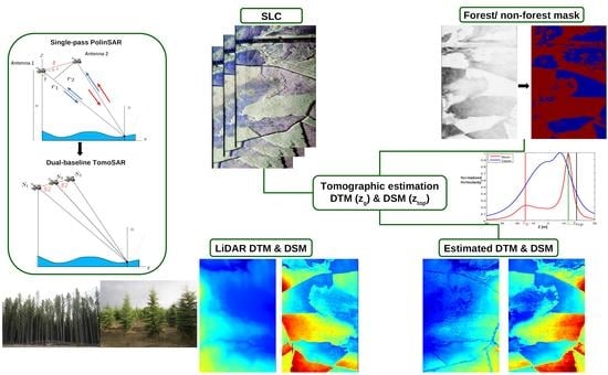
2.3. Single-Pass Dual-Baseline Tomographic Configuration

TomoSAR, with an additional aperture in elevation formed by multiple acquisitions, is able to reconstruct the 3D structures of semi-transparent media, and in particular forests. Tomographic techniques can provide very good estimates of tree heights and underlying ground topography using repeat-pass Fully Polarimetric (FP) datasets [8,16].
The acquisition system used in this study offers the possibility to acquire Multi-Baseline Polarimetric Interferometric SAR (MB-PolInSAR) data during a single pass of the airborne platform. This advanced functionality is based on the sequential use of two sets of antenna elements having each transmit and receive capabilities. This sequence of acquisitions is illustrated in Figure 3, and it may be described as follows. A signal is first emitted by Antenna 1 at position S 1 and the response of the scene is received by both Antenna 1 and Antenna 2. The corresponding signals are called y 1 and y 2 . Then, a signal is emitted by Antenna 2 at position S 2 and the scene echo is measured by the same antenna, which is called y 3 . Let ϕ i , j represent the phase delay between the signals y i and y j due to the distance travelled by the measured wave; according to the configuration sketched in Figure 3, one can then write
ϕ 1 , 2 = 2 π λ ( 2 r 1 2 r 2 ) = 4 π λ ( r 1 r 2 ) , ϕ 1 , 3 = 2 π λ ( r 1 r 2 ) = 4 π λ ( r 1 r 2 ) 2
The relationship between the components of ϕ i , j related to the acquisition geometry is implied by the specific ping-pong, non-ping-pong measurement sequence. Such an acquisition is equivalent to using a three-element equi-spaced array, with an inter-element spacing equal to B / 2 , as shown in Figure 3. The resulting dual-baseline interferometric and polarimetric SAR system may be used to reconstruct the scene 3D reflectivity, as shown in [17] for urban areas.
Compared to a classical repeat-pass acquisition system, the dual-baseline TomoSAR configuration used here presents several advantages. First, it measures a complete MB-InSAR set within a single flight, instead of three in the repeat-pass configuration, and it can significantly reduce the experimental cost and efforts. Second, single-pass acquisitions are only marginally affected by temporal decorrelation, which may reveal a very limiting factor, particularly over forested areas whose response is known to be highly affected by the presence of wind. The main drawback linked to the use of a single-pass tomographic system concerns the restricted range of baseline B, which may be physically realized on an airborne platform. In the experimental results of this paper, the baseline B was set to 3.5 m, and the corresponding vertical resolution δ z varied from 13 m in near range to 84 m in far range, as shown in Figure 4.
The correlation properties of the images acquired by the system on the test site are illustrated in Figure 5. One can note that the level of correlation of the InSAR data pair corresponding to the smaller baseline, B / 2 , is characterized by high values, even over densely vegetated areas, and does not depend on the considered polarimetric channel. In the larger baseline case, B, volume decorrelation is observed in near range and becomes negligible as range increases, with a high level of correlation in mid and far range. These correlation maps are characteristic of an absence of temporal decorrelation.

3. Estimation of Forest DTM and DSM

Polarimetric tomographic processing techniques, adapted to dual-baseline interferometric and polarimetric SAR system, are applied for estimating the forest DTM, DSM and tree heights.

3.1. Polarimetric Tomographic Processing

In the case of an MB-InSAR acquisition, considering an azimuth-range resolution cell that contains n s backscattering contributions from scatterers located at different heights and assuming no decorrelation between the different acquisitions, the received data vector, y C M × 1 , can be formulated as:
y ( l ) = i = 1 n s s i a ( z i ) + n ( l ) = A ( z ) s + n ( l )
where l = 1 , , L indicates one of the L independent realizations of the signal acquisition, also called looks. The source signal vector, s = [ s 1 , , s n s ] T , contains the unknown complex reflection coefficient of the n s scatterers, and n C M × 1 represents the complex additive noise, assumed to be Gaussianly distributed with zero mean variance σ n 2 , and to be white in time and space, i.e., n N ( 0 , σ n 2 I ( M × M ) ) and E ( n ( l ) n ( k ) ) = σ n 2 I ( M × M ) δ l , k . The steering vector a ( z ) contains the interferometric phase information associated to a source located at the elevation position z above the reference focusing plane and is given by:
a ( z ) = [ 1 , exp ( j k z 2 z ) , , exp ( j k z M z ) ] T
where k z j = 4 π λ B j r 1 sin θ is the two-way vertical wavenumber between the master and the jth acquisition tracks, with the corresponding perpendicular baseline B j . The carrier wavelength is represented by λ , whereas θ stands for the incidence angle and r 1 is the slant range distance between the master track and the scatterer. The steering matrix A ( z ) consists of n s steering vectors A ( z ) = [ a ( z 1 ) , , a ( z n s ) ] with z = [ z 1 , , z n s ] T .
The polarimetric response of a scatterer may be represented by a N P -element data vector, v, containing the complex scattering coefficients measured for different transmitted and received polarization states. In a monostatic configuration, and using the well-known Pauli polarization basis [18], this vector is written as v = 1 2 [ S hh + S vv , S hh S vv , 2 S hv ] , where S xy , with x and y equal to h or v, represents one elements of the ( 2 × 2 ) scattering matrix S. Signals measured in an MB-PolInSAR configuration are then gathered in an N P M -element polarimetric tomographic received signal, y P , formed by stacking the TomoSAR responses for each polarization channel, as y P = [ y 1 T , y N P T ] T C N P M × 1 , where y q C N P M × 1 represents the MB-InSAR response for the qth polarimetric channel, i.e., [ y q ] j = [ v j ] q ( q = 1 , , N P ). Using this convention, the polarimetric steering vector of the ith source, i.e., the ideal interferometric response with unitary polarimetric target vector k i , is given by
a ( z i , k i ) = I N P × N P a ( z i ) k i = B a ( z i ) k i
where k i is the polarimetric target vector of the ith source and K = [ k 1 , , k n s ] . Similar to the single polarization expression in (2), the received MB-PolInSAR data y P ( l ) is given by
y P ( l ) = i = 1 n s s i a ( z i , k i ) + n ( l ) = A ( z , K ) s ( l ) + n ( l ) C 3 M × 1
where s ( l ) C n s × 1 represents a realization of the complex amplitude of the ith source. The reflectivity, scattering vector and height σ i , k i , z i of each source, may be estimated from R P = E ( y P ( l ) y P ( l ) ) , but in practice these parameters are estimated from the L look estimate of the data covariance matrix R ^ P = 1 L 1 L y P ( l ) y P ( l ) using polarimetric tomographic techniques. Compared to single polarization tomography, the use of several polarization channels results in an undeniable increase of performance improvement for recovering the physical features of the observed medium. Polarimetric diversity also provides a better estimation accuracy for polarimetric tomographic estimators than single polarization ones, as shown in [17,19]. Various polarimetric tomographic techniques are listed in [17] where their performance is compared in details.

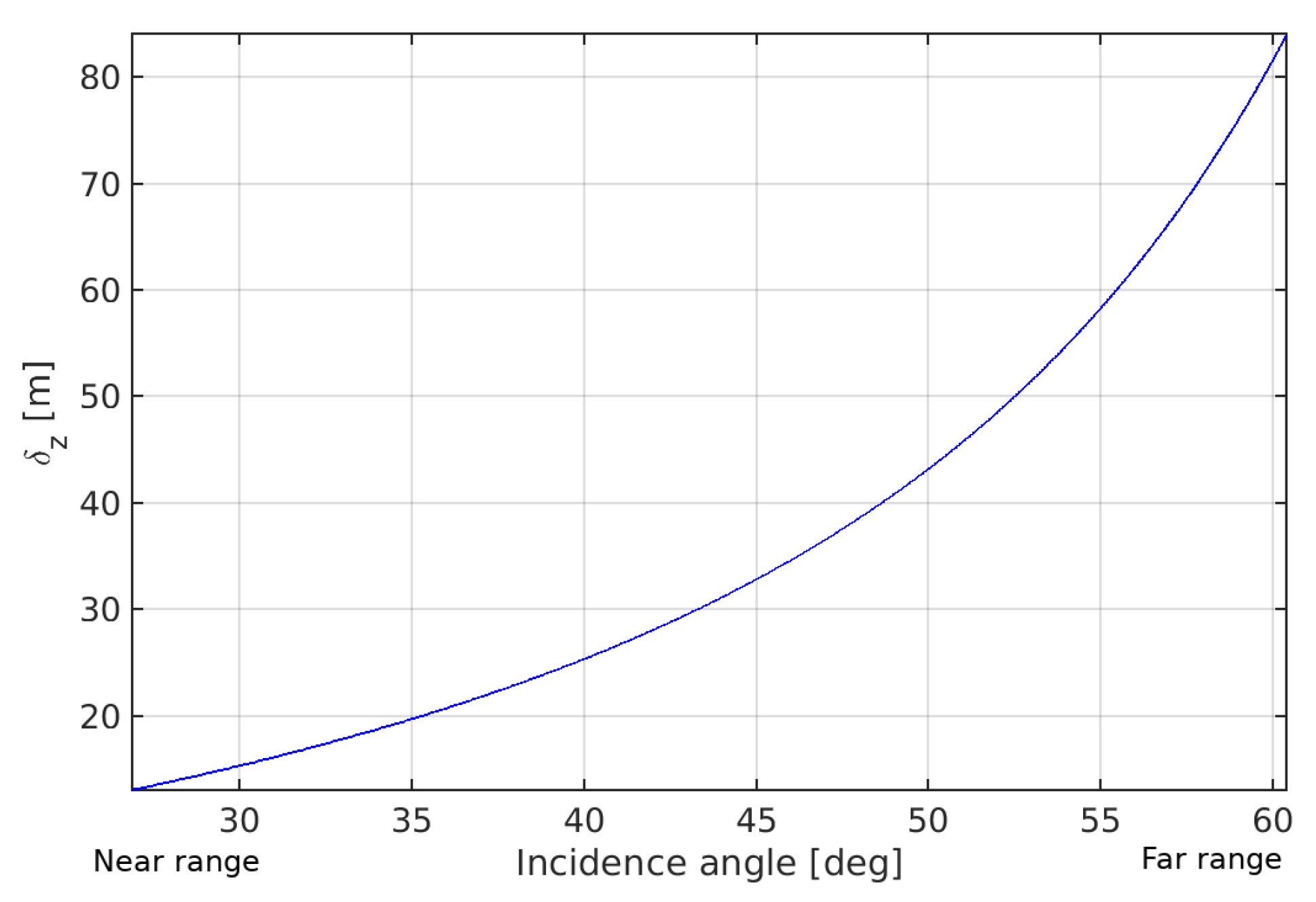
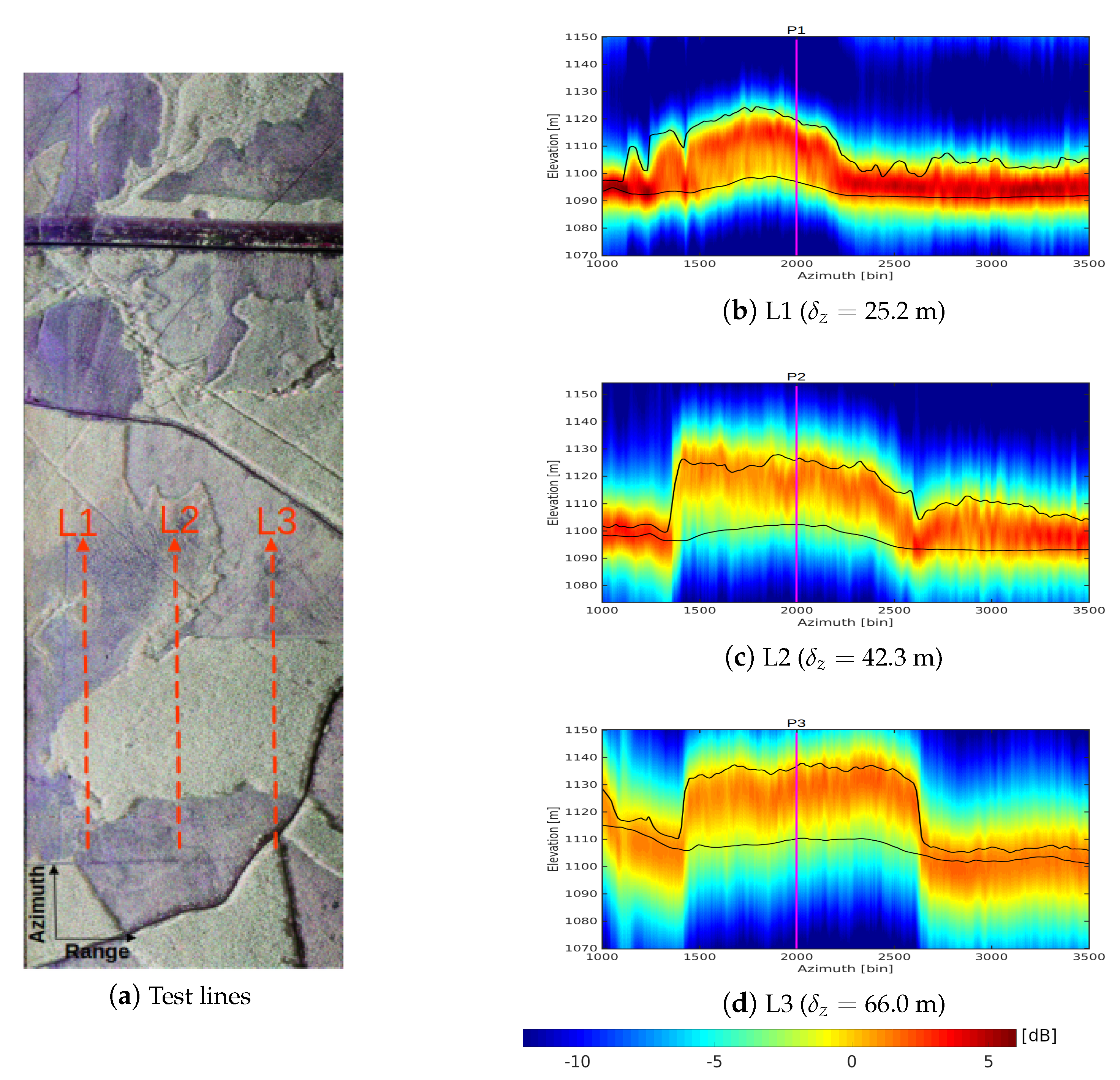
3.2. Limitation Due to a Coarse Vertical Resolution

Natural volumes, such as forest canopies, being composed of a large number of scatterers whose responses cannot be discriminated by the resolution of analysis, their scattering patterns are generally considered as a vertical density of random or speckle-affected reflectivity. To estimate this type of power spectral density, the classical polarimetric tomographic estimator, P-Capon, is usually a good choice, and it is well appreciated for the characterization of forests [14,16], as it allows estimating the vertical reflectivity with an improved resolution with respect to the traditional Beamforming technique. It is non-parametric and estimates the reflectivity at a given elevation as:
P C ( z ) = max k P C ( z , k ) = 1 λ m i n ( B a ( z ) R ^ P 1 B a ( z ) ) k ^ C i = e m i n ( B a ( z ^ i ) R ^ P 1 B a ( z ^ i ) )
where k ^ C i represents the polarimetric target vector at the height z i , λ m i n is the smallest eigenvalue of B a ( z ) R ^ P 1 B a ( z ) and its corresponding eigenvector it e m i n .
As mentioned above, the dual-baseline TomoSAR configuration used in this study, possesses a vertical resolution ranging from 13 m in near range up to 84 m in far range, whereas the studied forest stands have tree heights varying from 10 to 30 m. Despite the known capability of Capon for improving the resolution of spectral analysis with respect to the classical Fourier or Beamforming method, difficulty may arise with respect to a precise characterization of the forest stands using the present TomoSAR configuration. Three test lines are respectively taken at near, mid and far range, as shown in Figure 6a, to evaluate the performance of Capon tomograms for estimating ground and tree top elevations. The resulting P-Capon tomograms in Figure 6 cannot be used to precisely characterize the forest structures in the vertical direction. Due to the resolution limitation, the profiles of vertical reflectivity over forested areas are generally composed of a single lobe merging ground and volume contributions, as shown with the normalized vertical reflectivity profiles given in Figure 7.

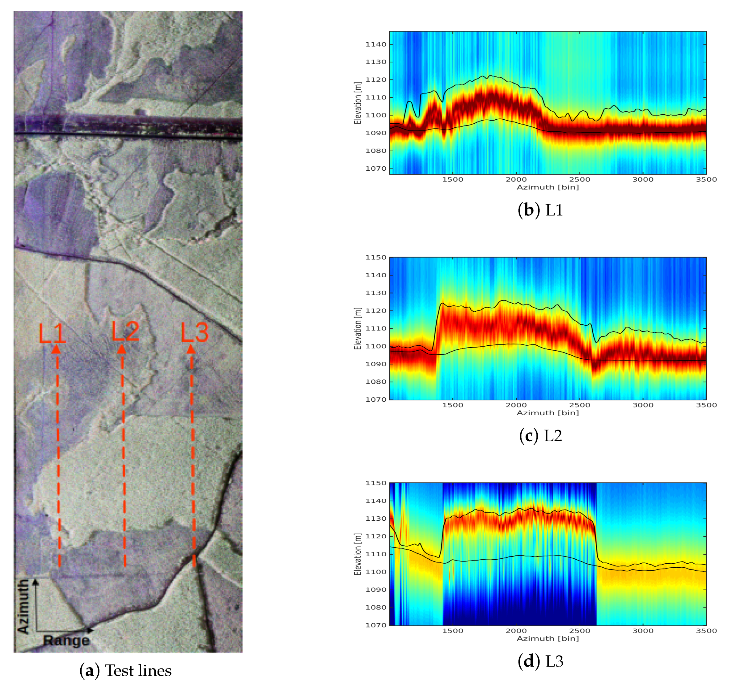
3.3. Proposed Solution Based on High-Resolution Spectral Analysis

High-Resolution (HR) spectral analysis techniques are able to estimate the elevation of well-localized contributions with a very high precision, that does not depend on the signal-to-noise ratio, but rather on the quality of the estimate of the data covariance matrix [20]. As illustrated in [11], HR techniques are not adapted to the characterization of distributed, continuous and speckle-affected densities of reflectivity, such as those corresponding to a forest response. Over such media, HR techniques provide estimates whose elevation is randomly distributed within the forest limits, as shown in [21]. Nevertheless, in the case of very coarse vertical resolution, it is very likely that the density of reflectivity of a forest can be approximated by two well-localized, i.e., Dirac-like, contributions. The first one is the ground response and contains the echoes directly reflected by the underlying ground as well as those corresponding to double-bounce reflection between the ground and tree trunks. The second one corresponds to the canopy, whose reflectivity profile vertical spread is much smaller than its physical extent, due to the extinction, and whose thickness remains by far inferior to the vertical resolution of the tomographic analysis. Under these assumptions, HR techniques may hence be used to estimate the ground elevation as well as the phase center of the canopy, as two well localized contributions.
Most HR polarimetric tomographic estimators are multi-dimensional approaches, which provide precise estimates of elevation and polarimetric parameters, even for coherent scatterers, as demonstrated in [17]. Nevertheless, multi-dimensional approaches usually suffer from a high computational complexity, and, to perform tomographic processing over a large forested area, a mono-dimensional HR approach is computationally attractive. The P-MUSIC technique is hence a good choice to localize the phase centers of the ground ( z g ) and volume ( z v ) scattering contributions in the vertical direction. Its criterion is given by:
P M ( z ) = max k P M ( z , k ) = 1 λ m i n ( B a ( z ) E ^ n E ^ n B a ( z ) ) k ^ M i = e m i n ( B a ( z ^ i ) E ^ n E ^ n B a ( z ^ i ) )
where the noise subspace E n = [ e n s + 1 , , e N P M ] is spanned by the eigenvectors corresponding to the N P M n s smallest eigenvalues of R P , assuming a number of sources equal to n s .
To estimate the ground and volume phase centers in elevation, one may naturally set n s = 2 . Indeed, the results given in Figure 8 indicate that, with such a parameterization, the P-MUSIC technique cannot precisely estimate the phase centers of ground and volume contributions in elevation. This is due to the fact that the covariance matrices of polarimetric responses of ground and canopy contributions have a rank larger than 1 and cannot be well described by a single target vector as in (7).

3.3.1. Model Order Selection for Ground and Volume Separation

In the general TomoSAR case, i.e., without any particular assumption of the source signal statistics, M acquisitions, composed of N P polarimetric channels, may be used to reconstruct up to M 1 sources having equal polarimetric responses and up to N P M 1 sources having all different polarimetric patterns. Considering ground and canopy polarimetric covariance matrices having full rank, i.e., occupying each a subspace of dimension equal to 3, the number of selected sources should be at least 4, i.e., n s 4 . Examples computed for n s > 2 , in Figure 9, demonstrate that the ground and volume phase centers can be separated by the P-MUSIC estimator with n s = 4 , in Figure 9c, whereas a better quality of tomographic focusing is provided by n s = 5 in Figure 9d. The model order n s = 5 is selected for the tomographic processing of forested areas in this paper.
To confirm this finding, a dual-baseline L-band polarimetric dataset is simulated over a homogenous forested area with varying forest parameters and ground conditions, using the PolSARproSIM software [22]. The resulting Pauli-coded images and the corresponding coherences are shown in Figure 10, with the PolSARproSIM parameters given in Figure 10a. The P-Capon technique and P-MUSIC estimator are both applied to the simulated dataset. Considering an intermediate ground roughness, i.e., Roughness = 4, the P-Capon method and P-MUSIC estimator with n s = 2 are able to estimate the ground and volume phase centers in the vertical direction, as shown in Figure 11b,e. Nevertheless they cannot localize the ground scattering contribution for rough surfaces (Figure 11c,d,f,g). With a model order increased to 4, the phase centers of ground and volume contributions are precisely estimated by the P-MUSIC technique, even for very rough surfaces, as illustrated in Figure 11h–j. These results from simulated data further validate the above empirical approach for model order selection.

3.3.2. Tree Height Tomographic Estimation Approach

As described above, the P-MUSIC spectral estimation technique is able to accurately estimate the ground elevation as well as the vertical position of the canopy volume phase center. To estimate the tree top elevation, a technique based on the estimate of the vertical reflectivity density provided by the P-Capon technique, formerly used in [8,14,23], and suggested by the profiles given in Figure 7, is adopted. The tree top height, z t o p , is estimated as the elevation so that P c ( z t o p ) = P c ( z v ) 3 , with z t o p > z v , as illustrated in Figure 12. The tree height h t r e e can be obtained in such a way: h t r e e = z t o p z g .
To demonstrate the effectiveness of the proposed approach, the ground topography and tree top heights are estimated for three test lines, as shown in Figure 13. The estimated elevations for the underlying ground and forest top show an excellent match with LiDAR-derived estimates.
This technique is then applied to the whole test site so as to map the forest DTM, DSM and tree heights.

4. Forest/Non-Forest Mapping for Model Order Selection

Forest/non-forest Mapping (FM) is generally required for GIS products related to forest characterization. The quality of this forest mapping is relevant to the final accuracy of forest-related variables. In this paper, FM is required to adequately set the model order of HR tomographic processing. Over non-forested area, the only scattering contribution to be estimated is the ground response, and n ^ s = 1 . Over forested areas, according to the study presented in the previous section, n ^ s = 5 is used. Forest mapping is achieved using the PolInSAR correlation information between y 1 and y 2 , i.e., using the larger baseline. The magnitude and phase of γ o p t 1 , defined as the optimal PolinSAR coherence, i.e., the coherence estimated over the polarimetric channel leading to the maximum magnitude, defined by Cloude and Papathanassiou [24] and studied in detail by Ferro-Famil et al. [25], are shown in Figure 14.
The forest mask is derived by thresholding the magnitude of this optimal coherence, | γ o p t 1 | in the following way:
FM = 1 if | γ o p t 1 | < T 0 otherwise
The threshold value T = 0.93 is selected, and the resulting FM mask, shown in Figure 15d, is compared to the LiDAR-derived tree heights given in Figure 15b. A very good agreement is found between the FM mask of Figure 15d and the binary map of LiDAR tree heights larger than 10 m in Figure 15c. Such a map effectively corresponds to a forest/non-forest map of the test site.

5. Global Tomographic Processing over the Test Site

Based on the FM mask of Figure 15d, the model order is set to n s = 1 for non-forest areas and n s = 5 for forested areas. The proposed tomographic approach is applied over the test site of Edson. The resulting DTM and DSM are validated against LiDAR-derived measurements. The TomoSAR-estimated DTM in Figure 16a shows some boundary effects at non-forest/forest transitions, as well as a slight overestimation of the elevation of the underlying ground. Nevertheless, it globally coincides with the LiDAR-derived DTM, with a comparable high resolution. Figure 16b demonstrates the undeniable quality of estimated DSM compared to the LiDAR-derived one. Some underestimated TomoSAR-derived values indicated by red circles in Figure 16b may be due to the forest/non-forest mask errors, as suggested by Figure 16. Compared with the LiDAR-derived tree heights of Figure 16c, the proposed tomographic technique provides globally a good performance for forest height estimation, using a dual-baseline TomoSAR configuration formed by a single-pass PolInSAR system with a single physical baseline and an extremely coarse vertical resolution.
To provide a detailed quantitative evaluation of the estimated forest parameters, nine Regions of Interest (ROI) are selected over forested areas, as shown in Figure 17, each covering a 55 m × 55 m wide area. Statistical features of TomoSAR- and LiDAR-derived tree heights are calculated, for each ROI, as
m ^ X , i = 1 N i q R i x ^ X , q σ ^ X , i = 1 N i 1 q R i ( x ^ X , q m ^ X , i ) 2 with X = T o m o , L i d a r , x = h t r e e
where N i represents the number of pixels included in the ith ROI, R i , with i = 1 , , 9 , as listed in Table 1. To further assess the quality of the proposed technique, the differences between TomoSAR- and LiDAR-derived estimates are characterized by their first- and second-order moments, computed as
Δ x ^ q = x ^ T o m o , q x ^ L i d a r , q with x = z g , h t r e e m ^ Δ x i = 1 N i q R i Δ x ^ q σ ^ Δ x i = 1 N i 1 q R i ( Δ x ^ q m ^ Δ x i ) 2
Figure 18a reveals the estimated DTM has a quality comparable to the LiDAR-derived one, with an average overestimation of 0.87 m for these ROIs. The estimated tree heights demonstrate a bias less than 2 m for most ROIs, except for ROI 3 and ROI 6, as depicted in Figure 18b, and still achieve an average underestimation of 2.2 m, which is less than 10 % of the LiDAR-derived tree heights over most ROIs. One may consider the use of a dual-baseline single-pass TomoSAR configuration, i.e., of a minimal configuration, and the accuracy of estimated forest parameters is hence well appreciated.

6. Discussion

The forest DTM, DSM and tree heights estimated by the proposed tomographic approach, as displayed in Figure 16, indicates that the FM mask plays an important role in the forest estimation process. Patches of short vegetation may be identified in the LiDAR-derived DSM in Figure 15b, but not in the TomoSAR-derived one. This is due to the coherence-derived FM mask of Figure 15d, which excludes the trees with height larger than 10 m. Boundary effects between forests and bare areas are clearly shown by the estimated DTM at the Edson area in Figure 16a. As shown in the Pauli-coded image of this test site in Figure 15a, these boundary effects mostly happen at the shadow areas where the underlying DTM cannot be reconstructed due to low SNR. It may hence be reasonable to remove the boundary areas and then interpolate DTM and DSM to improve the final estimates.
From the methodological perspective, the proposed hybrid tomographic approach provides an excellent performance for this dataset, using a model order selected in an adaptive way, as described in Section 3.3.1.
From the system perspective, unlike from other single-baseline PolInSAR systems, this specific system combines both ping-pong and non-ping-pong InSAR modes simultaneously, and it results in a dual-baseline configuration that permits tomographic processing. Moreover, this system performs the data acquisitions in a single flight, which effectively reduces the technical effort and cost for forest monitoring, and is intrinsically robust to temporal decorrelation, resulting in a better 3D reconstruction of forests.

7. Conclusions

This paper addresses forest height estimation for boreal forests at the test site of Edson in Alberta, Canada, using Intermap’s single-pass PolInSAR dataset. This particular dataset is acquired by using both ping-pong and non-ping-pong modes, which permits to form a dual-baseline TomoSAR configuration, i.e., an extreme configuration of tomographic processing. Mono-dimensional tomographic techniques are preferred in this paper, considering computational complexity of tomographic processing over a large forested area. Classical polarimetric Capon and MUSIC tomographic estimators are discussed and applied to the test data. The P-Capon technique provides a robust estimate of the vertical distribution of the back scattered power over forested areas, but it cannot recover the underlying ground elevation due to its limited resolution. The P-MUSIC technique with an appropriate model order is able to separate the volume and ground contributions in this specific low resolution configuration, but it cannot recover the tree top height. To overcome these limitations, a tomographic approach is proposed, based on P-MUSIC and P-Capon techniques, which provides excellent performance for forest parameter estimation, including DTM, DSM and tree heights. In conclusion, this paper demonstrates the undeniable potential of single-pass L-band PolInSAR system for forest height estimation, using simple tomographic techniques. Besides, this system, characterized by its single-pass configuration, can effectively fight against the temporal decorrelation of forests, leading to a potential solution for the 3D forest imaging from space.

Author Contributions

Conceptualization, methodology and validation, Y.H.; preparation of SAR data and LiDAR measurements, validation and review, Q.Z.; and scientific discussion, review and editing, L.F.-F. All authors have read and agreed to the published version of the manuscript.

Funding

This research was funded in part by the Alberta Innovates Technologies Future-R&D Associates program and in part by ANR (the French National Research Agency) and DGA (Direction Générale de l’Armement) under the ALYS project ANR-15-ASTR-0002.

Acknowledgments

The authors would like to thank Terrapoint Canada Inc. for providing the LiDAR ground truth data, and Valtus Imagery Services for providing the air photos.

Conflicts of Interest

The authors declare no conflict of interest.

Abbreviations

The following abbreviations are used in this manuscript:
PolInSARPolarimetric Interferometric SAR
TomoSARSAR Tomography
DTMDigital Terrain Model
DSMDigital Surface Model

References

  1. Frolking, S.; Palace, M.W.; Clark, D.B.; Chambers, J.Q.; Shugart, H.H.; Hurtt, G.C. Forest disturbance and recovery: A general review in the context of spaceborne remote sensing of impacts on aboveground biomass and canopy structure. J. Geophys. Res. Biogeosci. 2009, 114. [Google Scholar] [CrossRef]
  2. Treuhaft, R.; Siqueira, P. Vertical structure of vegetated land surfaces from interferometric and polarimetric radar. Radio Sci. 2000, 35, 141–178. [Google Scholar] [CrossRef] [Green Version]
  3. Papathanassiou, K.P.; Cloude, S.R. Single baseline polarimetric SAR interferometry. IEEE Trans. Geosci. Remote Sens. 2001, 39, 2352–2363. [Google Scholar] [CrossRef] [Green Version]
  4. Cloude, S.R.; Papathanassiou, K.P. Three-stage inversion process for polarimetric SAR interferometry. IEE Proc. Radar Sonar Navig. 2003, 150, 125–134. [Google Scholar] [CrossRef] [Green Version]
  5. Tebaldini, S. Forest Structure Retrieval from Multi-Baseline SARs. In Remote Sensing of Biomass; Fatoyinbo, T., Ed.; IntechOpen: Rijeka, Croatia, 2012; Chapter 2. [Google Scholar]
  6. Pardini, M.; Papathanassiou, K. On the Estimation of Ground and Volume Polarimetric Covariances in Forest Scenarios with SAR Tomography. IEEE Geosci. Remote Sens. Lett. 2017, 14, 1860–1864. [Google Scholar] [CrossRef] [Green Version]
  7. Ferro-Famil, L.; Huang, Y.; Pottier, E. Principles and Applications of Polarimetric SAR Tomography for the Characterization of Complex Environments. In VIII Hotine-Marussi Symposium on Mathematical Geodesy; Springer: Berlin/Heidelberg, Germany, 2015; pp. 1–13. [Google Scholar] [CrossRef]
  8. Huang, Y.; Ferro-Famil, L.; Lardeux, C. Polarimetric SAR tomography of tropical forests at P and L-band. In Proceedings of the 2011 IEEE International Geoscience and Remote Sensing Symposium, Vancouver, BC, Canada, 24–29 July 2011; pp. 1373–1376. [Google Scholar]
  9. Li, X.; Liang, L.; Guo, H.; Huang, Y. Compressive Sensing for Multibaseline Polarimetric SAR Tomography of Forested Areas. IEEE Trans. Geosci. Remote Sens. 2016, 54, 153–166. [Google Scholar] [CrossRef]
  10. Aghababaei, H.; Ferraioli, G.; Ferro-Famil, L.; Huang, Y.; Mariotti D’Alessandro, M.; Pascazio, V.; Schirinzi, G.; Tebaldini, S. Forest SAR Tomography: Principles and Applications. IEEE Geosci. Remote Sens. Mag. 2020, 8, 30–45. [Google Scholar] [CrossRef]
  11. Huang, Y.; Levy-Vehel, J.; Ferro-Famil, L.; Reigber, A. Three-Dimensional Imaging of Objects Concealed Below a Forest Canopy Using SAR Tomography at L-Band and Wavelet-Based Sparse Estimation. IEEE Geosci. Remote Sens. Lett. 2017, 14, 1454–1458. [Google Scholar] [CrossRef]
  12. Lee, S.; Pardini, M.; Kugler, F.; Papathanassiou, K.; Hajnsek, I. PolInSAR forest height inversion by means of L-band F-SAR data. PolInSAR Workshop 2013. [Google Scholar]
  13. Hajnsek, I.; Kugler, F.; Lee, S.K.; Papathanassiou, K.P. Tropical-Forest-Parameter Estimation by Means of Pol-InSAR: The INDREX-II Campaign. IEEE Trans. Geosc. Remote Sens. 2009, 47, 481–493. [Google Scholar] [CrossRef] [Green Version]
  14. Tebaldini, S.; Rocca, F. Multibaseline Polarimetric SAR Tomography of a Boreal Forest at P- and L-Bands. IEEE Trans. Geosci. Remote Sens. 2012, 50, 232–246. [Google Scholar] [CrossRef]
  15. Mercer, B.; Zhang, Q.; Schwaebisch, M.; Denbina, M. 3D Topography and Forest Recovery from An L-Band Single-Pass Airborne PolInSAR System. In Proceedings of the 2009 IEEE International Geoscience and Remote Sensing Symposium, Cape Town, South Africa, 12–17 July 2009. [Google Scholar]
  16. Tebaldini, S. Algebraic Synthesis of Forest Scenarios From Multibaseline PolInSAR Data. IEEE Trans. Geosc. Remote Sens. 2009, 47, 4132–4142. [Google Scholar] [CrossRef]
  17. Huang, Y.; Ferro-Famil, L. 3-D Characterization of Urban Areas Using High-Resolution Polarimetric SAR Tomographic Techniques and a Minimal Number of Acquisitions. IEEE Trans. Geosci. Remote Sens. 2020, 1–18. [Google Scholar] [CrossRef]
  18. Lee, J.S.; Pottier, E. Polarimetric Radar Imaging: From Basics to Applications; CRC Press: Chicago, IL, USA, 2008. [Google Scholar]
  19. Huang, Y.; Ferro-Famil, L.; Reigber, A. Under-Foliage Object Imaging Using SAR Tomography and Polarimetric Spectral Estimators. IEEE Trans. Geosci. Remote Sens. 2012, 50, 2213–2225. [Google Scholar] [CrossRef] [Green Version]
  20. Stoica, P.; Nehorai, A. MUSIC, Maximum likelihood, and Cramer-Rao Bound: Further Results and Comparisons. IEEE Trans. Acoust. Speech Signal Process. 1990, 38, 2140–2150. [Google Scholar] [CrossRef]
  21. Nannini, M.; Scheiber, R.; Moreira, A. Estimation of the Minimum Number of Tracks for SAR Tomography. IEEE Trans. Geosc. Remote Sens. 2009, 47, 531–543. [Google Scholar] [CrossRef]
  22. Williams, M.; Pottier, E.; Ferro-Famil, L.; Allain, S.; Cloude, S.; Hajnsek, I.; Papathanassiou, K.; Moreira, A.; Minchella, A.; Desnos, Y.L. Forest Coherent SAR Simulation within PolSARPro: An Educational Toolbox for PolSAR and PolInSAR Data Processing. In Proceedings of the Asian Conference on Remote Sensing, Kuala Lumpur, Malaysia, 12–16 November 2007. [Google Scholar]
  23. Zhang, Q.; Huang, Y.; Schwaebisch, M.; Mercer, B.; Wei, M. Forest height estimation using single-pass dual-baseline L-band PolInSAR Data. In Proceedings of the 2012 IEEE international geoscience and remote sensing symposium, Munich, Germany, 22–27 July 2012. [Google Scholar]
  24. Cloude, S.R.; Papathanassiou, K.P. Polarimetric SAR interferometry. IEEE Trans. Geosci. Remote Sens. 1998, 36, 1551–1565. [Google Scholar] [CrossRef]
  25. Ferro-Famil, L.; Lee, J.; Pottier, E. Unsupervised Classification of Natural Scenes from Polarimetric Interferometric SAR Data. In Frontiers of Remote Sensing Information Processing; World Scientific Publishing: Singapore, 2003. [Google Scholar]
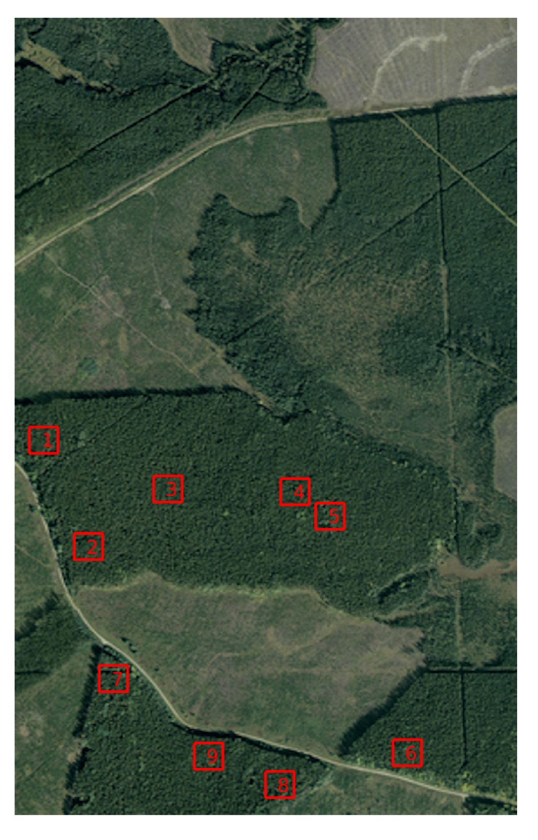
Figure 1. Illustration of the Edson test site.
Remotesensing 13 00487 g001
Figure 2. LiDAR-derived tree heights over Edson (courtesy Terrapoint Canada).
Remotesensing 13 00487 g002
Figure 3. Illustration of transmit–receive modes and equivalent dual-baseline TomoSAR configuration. S 1 and S 2 are the real positions of Antenna 1 and Antenna 2, whereas S 3 is the virtual resulting position.
Remotesensing 13 00487 g003
Figure 4. Tomographic resolution δ z w.r.t range.
Remotesensing 13 00487 g004
Figure 5. InSAR coherences over the test site.
Remotesensing 13 00487 g005
Figure 6. P-Capon tomograms for test lines located in near, mid and far range, respectively. The black line is the LiDAR ground and tree top elevation estimates.
Remotesensing 13 00487 g006
Figure 7. Normalized vertical reflectivity profiles estimated by P-Capon technique at the locations indicated in Figure 6. Elevation here is measured with respect to the LiDAR ground elevation.
Remotesensing 13 00487 g007
Figure 8. P-MUSIC tomograms for test lines located in near, mid and far range, respectively. n s = 2 . The black line is the LiDAR ground and tree top elevation estimates.
Remotesensing 13 00487 g008
Figure 9. P-MUSIC tomograms with model order larger than 2. The black line is the LiDAR ground and tree top elevation estimates.
Remotesensing 13 00487 g009
Figure 10. Simulated dual-baseline FP data of forests. The illustrated Pauli-coded images are generated in the case of Roughness = 4.
Remotesensing 13 00487 g010
Figure 11. P-Capon and P-MUSIC tomograms with n s = 2 and n s = 4 over a test line for different ground roughness: P-Capon (bd); and P-MUSIC (ej).
Remotesensing 13 00487 g011
Figure 12. Proposed tomographic approaches for estimation tree height.
Remotesensing 13 00487 g012
Figure 13. Ground topography and tree top heights estimated by the proposed tomographic approach. Background, P-Capon tomograms; gray line, estimated ground and tree top elevations; black line, LiDAR ground and tree top elevation estimates.
Remotesensing 13 00487 g013
Figure 14. γ o p t 1 map over the test site.
Remotesensing 13 00487 g014
Figure 15. Generated forest/non-forest mask.
Remotesensing 13 00487 g015
Figure 16. DSM, DTM and tree height maps estimated by the proposed tomographic technique and using LiDAR data.
Remotesensing 13 00487 g016
Figure 17. Location of ROIs.
Remotesensing 13 00487 g017
Figure 18. Statistical features of TomoSAR- and LiDAR-derived elevation estimates over different ROIs. The red bar has a length equal to 2 σ ^ Δ x i , the black cross mark indicates m ^ Δ x i and the green bar has a length equal to 2 σ ^ L i d a r , i , with i = 1 , , 9 .
Remotesensing 13 00487 g018
Table 1. TomoSAR- and LiDAR-derived tree height statistical descriptors.
ROI m ^ Tomo ± σ ^ Tomo (m) m ^ Lidar ± σ ^ Lidar (m)
124.57 ± 2.5926.39 ±0.72
222.40 ± 2.9023.71 ± 0.77
319.32 ± 1.8621.84 ± 0.38
418.10 ± 2.0819.95 ± 0.42
520.58 ± 1.7321.40 ± 0.72
621.68 ± 1.8826.36 ± 0.58
720.80 ± 3.5524.63 ± 0.94
824.33 ± 1.4323.80 ± 1.21
919.54 ± 1.4821.50 ± 0.68
Publisher’s Note: MDPI stays neutral with regard to jurisdictional claims in published maps and institutional affiliations.

