Estimation of Field-Level NO_x Emissions from Crop Residue Burning Using Remote Sensing Data: A Case Study in Hubei, China

Abstract

Crop residue burning is the major biomass burning activity in China, strongly influencing the regional air quality and climate. As the cultivation pattern in China is rather scattered and intricate, it is a challenge to derive an accurate emission inventory for crop residue burning. In this study, we proposed a remote sensing-based method to estimate nitrogen oxide (NO_x) emissions related to crop residue burning at the field level over Hubei, China. The new method considers differences in emission factors and the spatial distribution for different crop types. Fire radiative power (FRP) derived from moderate-resolution imaging spectroradiometer (MODIS) was used to quantify NO_x emissions related to agricultural biomass combustion. The spatial distribution of different crops classified by multisource remote sensing data was used as an a priori constraint. We derived a new NO_x emission database for Hubei from 2014 to 2016 with spatial resolution of 1 × 1 km. Significant seasonal patterns were observed from the NO_x emission database. Peak NO_x emission occurring in October was related to the residue burning in late autumn harvesting. Another peak was observed between January and April, which was due to the frequent burning of stubble before spring sowing. Our results were validated by comparing our emission inventory with geostationary satellite observations, previous studies, global fire emission database (GFED), NO₂ vertical column densities (VCDs) from ozone monitoring instrument (OMI) satellite observations, and measurements from environmental monitoring stations. The comparisons showed NO_x emission from GFED database was 47% lower than ours, while the evaluations from most of the statistical studies were significantly higher than our results. The discrepancies were likely related to the differences of methodology and data sources. The spatiotemporal variations of NO_x emission in this study showed strong correlations with NO₂ VCDs, which agreed well with geostationary satellite observations. A reasonable correlation between in situ NO₂ observations and our results in agricultural regions demonstrated that our method is reliable. We believe that the new NO_x emission database for crop residue burning derived in this study can potentially improve the understanding of pollution sources and can provide additional information for the design of pollution control measures.

1. Introduction

Agriculture is one of the most prominent sources of air pollution. Agricultural emissions mainly include emissions from nitrogen-rich fertilizers, natural emissions from crops, and emissions from crop residue burning. In the past two decades, open-field burning of crop residue has been controlled effectively due to the implementation of a sustainable development strategy and strict environmental protection policies. However, open burning in some rural areas is rather severe. These emissions play a crucial role in tropospheric ozone and secondary aerosol formation [1,2,3,4,5] (e.g., nitrogen oxides). Nitrogen oxide (NO_x) (NO_x ≡ NO + NO₂) is a major atmospheric pollutant, and a previous study demonstrated that NO_x concentration in Hubei is tripled during the crop residue burning seasons [6]. Therefore, an accurate estimation of NO_x emissions related to residue burning is essential for the investigation of impacts on regional air quality and design of environmental protection guidelines.

There are three major methods for the estimation of NO_x emission from crop residue burning. They are the statistical method based on field investigations [7,8,9,10,11,12], remote sensing detection of burned areas [6,13,14], and estimation of fire radiative power (FRP) from remote sensing observations [15,16,17,18]. The traditional statistically based method relies mainly on field investigations to obtain parameters including crop cultivation area, crop yield per unit area, grain/straw ratio, burning rate, and emission factor (EF). NO_x emissions can then be calculated using these statistical data. However, the statistical reports are likely to take in uncertainties during data collection, i.e., human errors. In addition, the temporal resolution of the method is rather low, i.e., once per year [7], which the temporal information is especially important for the modelling and real-time forecast of air pollution. Satellite remote sensing provides more insight information on burning activities. Most of these estimations from space are based on the observations of burned area using the formula introduced by Selier and Crutzen [19]. The total amount of dry matter in combustion is obtained by multiplying the burned area, biomass load, and combustion efficiency, and the emission can be calculated combining with the relative EFs [6,20,21,22]. The theoretical basis of this method is that the biomass consumed can be estimated from the traces of fires [23]. Nevertheless, the accuracy of burned area depends on the temporal resolution of the sensors and weather conditions. As a result, small-scale burnings are often omitted. Moreover, the biomass load and combustion efficiency are geographically heterogeneous, which introduce additional uncertainties. Several datasets of the statistics of burned area have been published, e.g., GBA2000 product [24], moderate resolution imaging spectroradiometer (MODIS) burned area product [13,14], and global fire emission database (GFED) [14]. The remote sensing-based FRP method was first proposed by Kaufman [25], being based on the fact that the variation of infrared radiation is proportional to the biomass combustion. In the past few decades, this method has become the mainstream for biomass burning emission estimation, as it overcomes the geographic heterogeneity. In addition, this method simplifies the data processing from fire radiative energy (FRE) to biomass burning emission and reduces the systematic errors in modelling [16]. The disadvantage of this method is that only the instantaneous burning conditions are recorded during the satellite overpass time. Due to incomplete information, i.e., lack of information on FRP diurnal variation, assumptions of the temporal variation are required [15,17,26]. However, most of the previous studies for the estimation of crop residue burning generally have adopted national or municipal statistical data [11,27,28,29] as an input and further reprojected the emissions into regular grids on the basis of the land cover data. As the spatiotemporal resolution of these datasets are rather low, the resolution of emission data is also coarse and often ignores the spatiotemporal variation on crop distribution [7,30].

This study focused on using fine scale crop distribution map to reduce the uncertainties of crop residue burning emission estimation. The MODIS FRP product was used to estimate burning emissions by assuming an optimized Gaussian function to approximate the fire diurnal cycle for Hubei. We compared our result to geostationary satellite observations, previous studies, GFED, ozone monitoring instrument (OMI) vertical column densities (VCDs), and in situ observations to evaluate the reliability and accuracy of this method.

The paper is organized as follows: Section 2 introduces our study area and the datasets used in this study. The procedures for the estimation of field-level crop residue burning emission are presented in Section 3. Section 4 shows the experimental results and comparative analysis. Section 5 concludes the major findings of this study.

2. Study Area and Materials

A brief description of the study area is presented in Section 2.1. The MODIS instrument and the level 3 product (MOD14A1/MYD14A1) used in emission approximation are described in Section 2.2. The crop distribution map used to allocate the emission to each crop type is presented in Section 2.3. Other auxiliary datasets used for validation, such as in situ observations, OMI tropospheric NO₂ columns, and Himawari-8 FRP data are presented in Section 2.4, Section 2.5 and Section 2.6, respectively.

2.1. Study Area

Hubei is located in the center of China with the east bounded by the Yangtze River delta and the west bounded by the Sichuan Basin (Figure 1). As it is surrounded by highly industrialized areas, air quality in Hubei can be strongly affected by pollution transport. The cultivated area of Hubei is 53,000 km², accounting for 28% of the total land area of the province. These cultivated areas are mainly allocated in Jianghan Plain and south-central Hubei. The major crops cultivated in Hubei are rice, wheat, corn, cotton, and rapeseed. The growth period of rice, corn, and cotton lies between May and October, while wheat and rapeseed mainly grow from mid-October to mid-May of the following year. In this study, we divided the 5 major crops into wintering crops (rapeseed and wheat) and spring sowing crops (rice, corn, and cotton).

2.2. The MODIS Instrument and Fire Product

Moderate-resolution imaging spectroradiometer (MODIS) is an important instrument carried by the Terra and Aqua in the U.S. Earth Observation System (EOS) program for observing biological and physical processes around the globe. Terra and Aqua together provide 4 observations every day at 10:30, 22:30 LT (local time) (Terra) and 01:30, 13:30 LT (Aqua). MODIS has 36 spectral bands covering wavelengths from 0.25 to 1 μm, providing observations of land and ocean temperatures, primary productivity, land surface coverage, clouds, aerosols, water vapor, and fires every 1–2 days.

MODIS thermal anomalies and fire daily Version 6 product were used in this study. The data were generated every 8 days at 1 km spatial resolutions as a level 3 product (MOD14A1/MYD14A1) [31]. These datasets were derived from MOD14 active fire product, which has been filtered by fire masks, pixel quality indicators, maximum FRP, and the position of the fire pixel within the scan [32].

2.3. Crop Distribution Map

Cropland distribution of Hubei is used to discriminate fires from different crop types. The dataset is in a spatial resolution of 30 m, which greatly improved the accuracy of the spatial emission distribution. The crop classification was conducted by using an advanced harmonic analysis on the basis of multisource remote sensing data, including hyperspectral and synthetic aperture radar (SAR) [33]. The major land cover types in Hubei are considered as paddy fields, dryland, non-cultivated lands, and water bodies. The major crop types in Hubei are rice, corn, cotton, wheat, and rapeseed. According to the crop phenology, we defined the spring sowing crops in paddy fields as being dominated by rice, while the dryland was defined as corn and cotton; the wintering crops are wheat and rapeseed both in paddy fields and dryland.

2.4. Environmental Monitoring Stations

In situ measurements were provided by the China National Environmental Monitoring Center (CNEMC). Approximately 1500 monitoring sites have been established in China for air quality monitoring. Data from monitoring station is hourly averaged ambient concentrations of NO₂. The NO₂ concentrations reported are closely related to the emission strength and strongly influenced by meteorological factors, other atmospheric chemistry processes, and sources other than residue burning. Therefore, we selected 3 rural stations for comparison where residue burning is expected to be the dominant NO_x source. The locations of the 3 stations are shown in Figure 1.

2.5. OMI NO₂ Product

Ozone monitoring instrument (OMI) is a passive nadir viewing satellite-borne imaging spectrometer [34] onboard the Earth Observing System’s (EOS) Aura satellite. The EOS Aura satellite orbits at an altitude of ∼710 km with a local Equator overpass time of 13:45 LT (local time). The instrument covers the wavelength ranges from 264 to 504 nm. The spatial resolution of OMI varies from ∼320 km² (at nadir) to ∼6400 km² (at both edges of the swath). The instrument scans along 14.5 sun-synchronous polar orbits per day, providing daily global coverage [35].

The NASA OMI NO₂ standard product version 3 [36,37], was used in this study. In the NO₂ product, slant column densities (SCDs) of NO₂ are derived from Earth’s reflected spectra in the visible range (402–465 nm) using an iterative sequential algorithm [38]. The OMI NO₂ SCDs are converted to VCDs by using the concept of air mass factor (AMF) [39]. The AMFs are calculated using NO₂ profiles simulated by the Global Modeling Initiative (GMI) chemistry transport model. The horizontal resolution of GMI is 1° (latitude) × 1.25° (longitude) [40].

2.6. Himawari-8 Fire Radiative Power Product

In this study, Himawari-8 Wild Fire (WLF) Level 2 product was used to evaluate the temporal variation of FRP approximated from MODIS observations. Advanced Himawari Imager (AHI) onboard the Himawari-8 satellite provides observations at 6 spectral channels. AHI provides imagery with high temporal resolution (≈10 min). The spatial resolution of Himawari-8 near-infrared and infrared bands is 2 km (sub-satellite point). Himawari-8 WLF Level 2 product provides observation of brightness temperature at 4 μm and 11 μm channel every 10 min. In this study, Himawari-8 WLF Level 2 product was developed by the Earth Observation Research Center (EORC) of the Japan Aerospace Exploration Agency (JAXA). Previous studies showed that FRP derived from AHI agrees well with MODIS observations, with a Pearson correlation coefficient of 0.9 [41]. Therefore, it can be used to evaluate the FRP diurnal cycle approximated from MODIS observations.

3. Methodology

The estimation of NO_x emission can be divided into two major steps. The first step is the estimation of fire radiative energy from MODIS FRP. The second step is the estimation of the corresponding emission factor of crops. Detailed description of each step is presented in the following.

3.1. Estimation of Fire Radiative Energy

FRE is an important factor to determinate the emission released during biomass burning. In this study, FRE was estimated by integrating the FRP (i.e., instantaneous FRE) over the life span of fire activities. However, MODIS only provides four measurements per day, which is not sufficient to capture the temporal variation of FRP for FRE calculation. As there is no satellite overpass during the peak burning hours, the most intensive burning period is likely to be ignored. To reconstruct the temporal variation of FRP, we assumed that the diurnal variation of background FRP follows a Gaussian function. The parameters of the Gaussian function can be approximated by the ratio of FRP between Terra and Aqua observations (abbreviated $FR{P}_{Terra}$/$FR{P}_{Aqua}$) [16]. This approach is well established and has already been applied to estimate biomass burning emission on a global extent [42], in India [42,43], in China [17], and in north China [9]. The modified Gaussian function can be written as follows:

$$FRE= {{\displaystyle \int }}_0^{24}FRP\left(t\right)dt$$

(1)

where FRE is the fire radiative energy, and FRP(t) represents the fire radiative power as a function of time t. Previous studies show that due to the differences in overpass time, the ratio of FRP between Terra and Aqua ($FR{P}_{Terra}$/$FR{P}_{Aqua}$) can be used to approximate the temporal variation of FRP [16,43]. In addition, it can be used to distinguish different types of fire [43]. The parameters b, σ, and h can be calculated from the $FR{P}_{Terra}$/$FR{P}_{Aqua}$, where b and σ denote the background and standard deviation of FRP diurnal variation, respectively. h is the local time with expected peak FRP. In this study, $FR{P}_{Terra}$/$FR{P}_{Aqua}$ were taken from thermal anomalies and fire product (MOD14A1/MYD14A1), which characterize the average FRP from Terra at 10:30, 22:30 LT (local time) and Aqua at 01:30, 13:30 LT (local time). The equations describing the relationship between the temporal variation of FRP and $FR{P}_{Terra}$/$FR{P}_{Aqua}$ are as follows [42]:

$$\mathrm{b}=0.86\times {\left(\frac{FR{P}_{Terra}}{FR{P}_{Aqua}}\right)}^2-0.52\times \frac{FR{P}_{Terra}}{FR{P}_{Aqua}}+0.08$$

(2)

$$\mathsf{\sigma }=3.89\times \frac{FR{P}_{Terra}}{FR{P}_{Aqua}}+1.03$$

(3)

$$\mathrm{h}=-1.23\times \frac{FR{P}_{Terra}}{FR{P}_{Aqua}}+14.57+\mathit{\Delta }$$

(4)

$$FRP\left(t\right)=\frac{FR{P}_{Aqua}\left(b+e^{-\frac{{\left(t-h\right)}^2}{2{\sigma }^2}}\right)}{\left[\left(b+e^{-\frac{{\left(13.5-h\right)}^2}{2{\sigma }^2}}\right)+\left(b+e^{-\frac{{\left(1.5-h\right)}^2}{2{\sigma }^2}}\right)\right]}$$

(5)

where $FR{P}_{Terra}$/$FR{P}_{Aqua}$ represents the daily average of each pixel. A local time parameter Δ (Δ = 4) is applied to adjust the difference of the FRP peak hour (h) to fit the diurnal curve in different regions [16]. In order to evaluate the application of the method mentioned above for Hubei, we compared the approximated temporal variation of FRP to observations from AHI. Details of the validation are shown in Section 4.4.1.

3.2. Crop-Specific Emission Factors

The emission factor of each crop type is the key parameter of the emission estimation. The production of NO_x is closely related to the nitrogen content, combustion temperature, and physical properties of crop residue [8]. EFs of different crops are usually estimated through combustion experiments in the laboratory.

Table 1. Nitrogen oxide (NO_x) emission factors (EFs) for various crop residue combustions (unit: $\mathrm{g}/\mathrm{kg}$ dry fuel).

Rice	Wheat	Corn	Cotton	Rapeseed	Reference
3.43$\pm$1.08	2.28$\pm$1.00	3.60$\pm$0.85	2.49$\pm$0.23		Cao et al. [49]
	3.3$\pm$1.7	4.3$\pm$1.8			Li et al. [50]
	1.14	1.27			Zhang et al. [51]
3.83$\pm$4.30		3.06$\pm$3.00			Zhang et al. [52]
1.42	3.31	4.3	2.68		Guan et al. [47]
1.42$\pm$0.46	1.19 ± 0.02			1.12 ± 0.15	Tang et al. [45]
	2.65	1.34	2.98	2.68	He et al. [46]
1.81 ± 0.09	1.12 ± 0.19	1.28 ± 0.04			Zhang et al. [8]
3.1	3.3	4.3	3.37	3.37	Li et al. [53]
1.81	3.3	3.36	2.98	1.12	Wu et al. [44]
1.42	1.19	3.36	2.98	1.12	this study

summarizes EFs from previous studies for major crop types in China. In this study, we adopted the EFs of corn and wheat from Wu et al. [44] and Tang et al. [45], respectively. The EF of cotton is 2.98 g/kg [44,46], rapeseed is 1.12 g/kg [44,45], and rice is 1.42 g/kg [45,47]. The farming pattern in rural areas of Hubei is dominated by small-holder farming individuals. The average farmland size is ~0.1 km², leading to scattered fields with large varieties of crops. Moreover, the spatial resolution of the crop distribution map used in this study was much higher than MODIS images. Therefore, the mixed crop types in a single grid were expected. In order to calculate the mixed emission factors of different crops, we developed a crop-mixed EFs scheme on the basis of the spatial distribution and phenological characteristics of crops. The crop-mixed EFs ($E{F}_{mixed}$) can be formulated by the following equation:

$$E{F}_{mixed}={\displaystyle \sum }_{i=1}^n{W}_{i}E{F}_i$$

(6)

where i is the crop type; n represents the total number of crop types in each pixel; and $W_i$ and $E{F}_i$ denote the weighting factor and EF of $cro{p}_i$, respectively. The area weighting factor $W_i$ is the percentage of the cultivated area of $cro{p}_i$ within a grid. These statistics are taken from the statistical yearbook [48].

3.3. Estimation of Field-Level NO_x Emissions

The NO_x emissions of crop residue burning at a specific grid (denoted by $Emissio{n}_{N{O}_x}$) can be calculated from FRE, emission factor ($E{F}_{mixed,N{O}_x}$), and conversion ratio. The emissions of each grid can be calculated as follows:

$$Emissio{n}_{N{O}_x}=FRE\times CR\times E{F}_{mixed, N{O}_x}$$

(7)

where FRE represents the total amount of fire radiative energy released within a burning activity, $E{F}_{mixed,N{O}_x}$ is the emission factor calculated according to Section 3.2, and CR represents the amount of NO_x emitted per MJ of FRE. Wooster et al. [18] reported a conversion ratio of 0.368 ± 0.015 kg/MJ, and that adopted by Freeborn et al. [54] was 0.453 ± 0.068 kg/MJ. In this study, we adopted the average CR of 0.41 ± 0.04 kg/MJ from the previous studies to convert FRE to emission from residue burning.

4. Results and Discussions

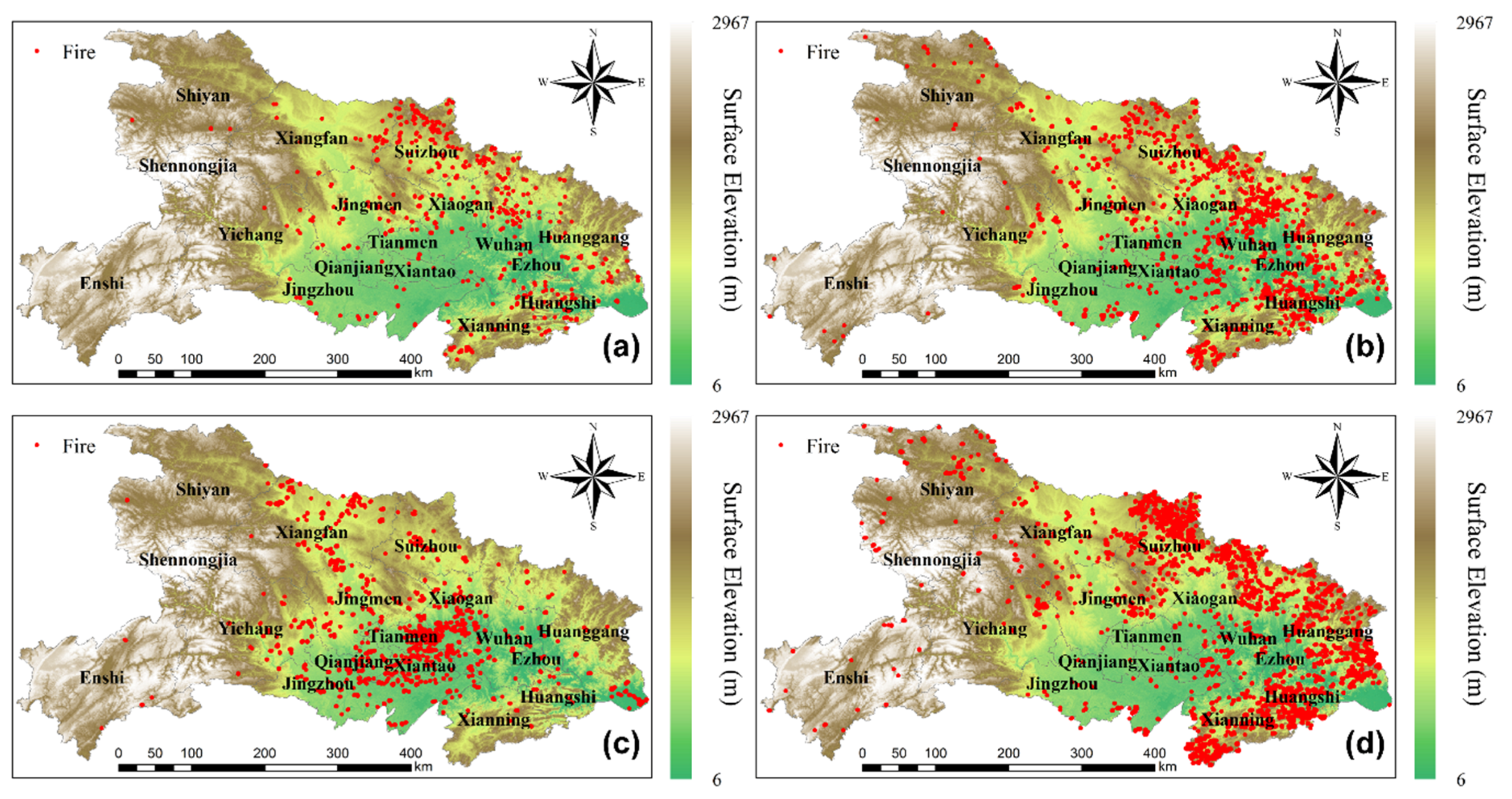
4.1. Fire Distribution for Different Landcovers

From January 2014 to December 2016, 11,324 fires were detected in Hubei by MODIS, including 5583 cases induced by the open-field burning of crop residue, accounting for 49% of the total fire counts. In 2014, 2015, and 2016, the number of fires detected in the agricultural region in Hubei was 2436, 1349, and 1798, respectively. Among them, 1719 cases were detected by Terra (overpass time at 10:30 local time) and 3864 were detected by Aqua (overpass time at 13:30 local time), which approximately accounted for 69% of agricultural fires. A larger number of fires from Aqua indicated that the crop residue in Hubei tended to be concentrated in the afternoon and evening. A possible reason is that people used to burn their crop residue in the time intervals when the law enforcement agencies were off duty. This phenomenon has also been reported in previous studies [9,17,41]. Figure 2 shows the daily and monthly (containing mean and standard deviation) variations of fire counts over lands covered with different crop types in Hubei from 2014 to 2016. Since the phenological periods of corn, cotton, and rice were similar, the monthly variations from November to April in the following year were alike. Fire counts over farming lands cultivated with corn and cotton were obviously higher than that of rice. For residue burning of rapeseed and wheat, fire counts appeared to be concentrated in the harvest season with major peaks around October. Non-agricultural fires showed a significant temporal pattern in that the fire activities in winter were more frequent than the other seasons. Relatively low precipitation and temperature play an important role in increasing number of wildfires in hilly regions. Higher demand of wood and coal burning for domestic heating also increases the chances of wildfires [55,56]. Comparing the temporal pattern of fire numbers in different years, we found that the residue burning occurred most frequently in 2014 and halved in 2015. Although the fire counts rose up again in early 2016, the burning activities during the autumn harvest were reduced. The policy regulation measures implemented in 2015 might have had a positive impact on the reduction of corresponding emissions. However, more evidence is needed to confirm the effectiveness of these control measures. Furthermore, the persistent wet weather in spring of 2015 also showed signs of reducing the burning in the open field [57].

Figure 3 shows the spatial distribution of four types of residue burning in Hubei from 2014 to 2016, including rice, corn and cotton, wheat and rapeseed, and non-cultivated land. The residue burning of rice was sparsely distributed in northern and southeastern Hubei. These farmlands are mainly lowlands located near rivers and along major highways due to the irrigation and transportation conveniences. Moreover, due to the lack of patrolling from the law enforcement agencies, people in the surrounding areas tend to disobey the regulation on prohibiting residue burning. In addition, the minimum fire numbers illustrated that a smaller proportion of rice residue (54%) are disposed by open field incineration. [53]. Corn and cotton residue burning in northern Hubei, at the junction of Wuhan and Huanggang cities, is predominantly caused by higher burning ratio [53,58] and large-scale cultivation of cotton and corn. Residue burning of wheat and rapeseed is primarily concentrated in Jianghan Plain, which is covered by a massive area of field crops and cereal production. Wintering crops such as wheat and rapeseed are planted in both dry and paddy fields corresponding to the crop-growing season from October to May in the following year. Consequently, the residue burning of wheat and rapeseed mainly occurred from May to October in the gap period of the sequential cropping. Burnings in non-cultivated land were mostly distributed in the north, northeast, and southeast of Hubei over hilly areas covered by dense evergreen needle leaved and evergreen broad-leaved forest. These are mostly remote areas with relatively sparse population. Nonetheless, most of the non-cultivated fires are caused by human activities, including burning during religious activities, burning grass, and unproductive fires.

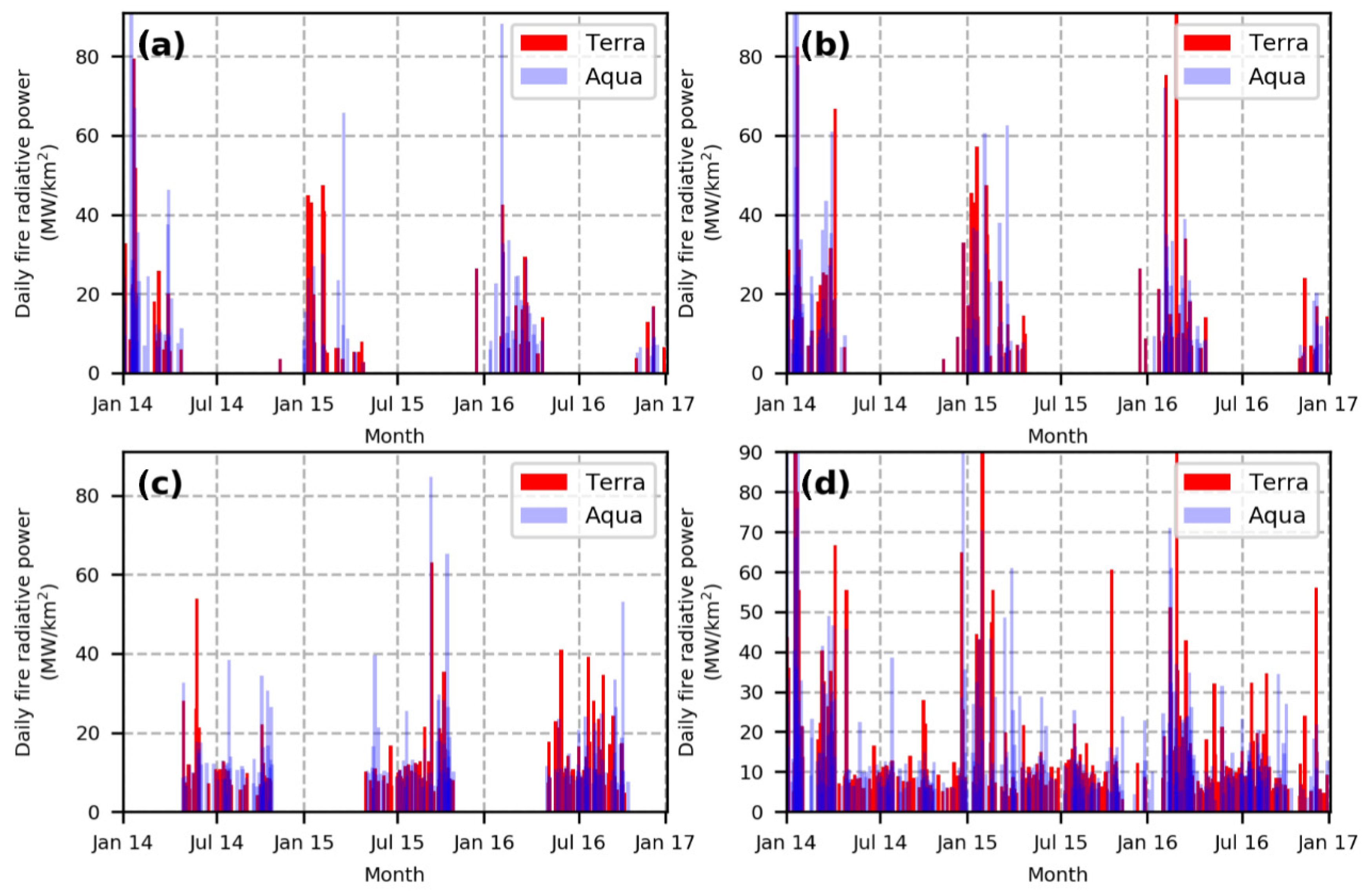
4.2. Daily Maximum Fire Radiative Power

To characterize the variation of daily maximum FRP of different crop residue in Hubei, we conducted statistical analysis by looking into the daily maximum FRP derived from MOD14A1/MYD14A1 products during 2014–2016 (Figure 4).

As shown in Figure 4a, 747 fire pixels were detected over rice cultivated lands. The majority of daily maximum FRP is usually associated with a peak from 30 to 70 MW/km². The mean and standard deviation of daily maximum FRP observed by Terra were 143 and 144 MW/km², respectively. The values from Aqua were 167 and 165 MW/km², respectively. Rice residue has the highest water content of 50–60% among the five staple crops. Therefore, rice residue burning tends to be incomplete combustion for which the burning process is often at a rather low temperature and low combustion efficiency [59].

For corn and cotton cultivated lands, 2301 fire pixels were obtained (Figure 4b). The range of peak daily maximum FRP varied from 30 to 70 MW/km². The mean and standard deviation of maximum daily FRP observed by Terra were 186 and 233 MW/km², respectively. The values from Aqua were 201 and 221 MW/km², respectively. The frequency histogram of daily maximum FRP between autumn harvest crops (rice, cotton, and corn) showed similar distributions.

As shown in Figure 4c, 2535 fire pixels in rapeseed and wheat cultivated lands were detected, of which the daily maximum FRP ranged from 64 to 104 MW/km². The mean and standard deviation of daily maximum FRP observed by Terra were 110 and 81 MW/km², respectively. The values from Aqua were 126 and 87 MW/km², respectively. Rapeseed and wheat are the second largest cultivation area in Hubei. They are densely cultivated along the shores of the Yangtze River. Moreover, the residue of rapeseed is rich in oil, which can be ignited easily. In addition, the calorific value of rapeseed residue is the second highest [60]. Therefore, the corresponding histogram of the daily maximum FRP shows the apparent characteristics of low standard deviation and high peak.

The non-cultivated land had a total of 5903 fire pixels (Figure 4d). The daily maximum FRP ranged from 67 to 107 MW/km². The mean and standard deviation of daily maximum FRP observed by Terra were 220 and 274 MW/km², respectively, while the values from Aqua were 267 and 331 MW/km² respectively. The histogram of daily maximum FRP of the non-cultivated land showed the largest standard deviation and mean. This was mainly due to the uncertainties of fuel types. For example, large-scale forest fires may present extremely high FRP, while the intensity of FRP caused by small-scale incineration of domestic waste is similar to open-field crop residue burning.

To conclude, the daily maximum FRP detected by Aqua was significantly higher than that of Terra, which indicated that crop residue burning in Hubei mainly occurred in the afternoon. Furthermore, except for rapeseed and wheat, the daily maximum FRP values in rice, corn, cotton, and non-cultivated land were highly scattered, as the standard deviations were higher than the mean value, which indicated the high complexity of the spatial distribution of crops in Hubei.

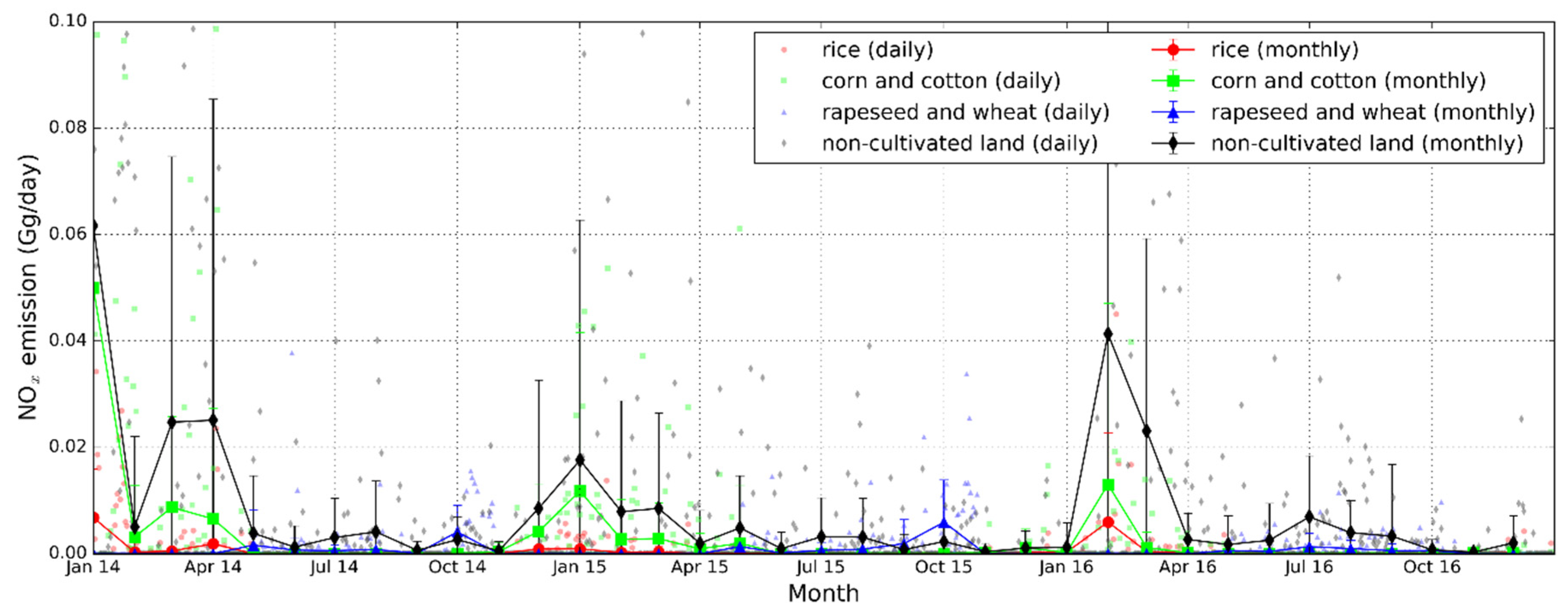
4.3. NO_x Emissions for Different Landcovers

Figure 5 illustrates the NO_x emission of crop residue burning from different land covers in Hubei during 2014–2016. The higher NO_x emission mainly occurred after the autumn harvest and before spring sowing, especially from mid-October to April of each year. A 79% reduction of NO_x emission from rice residue burning was observed from 0.79 Gg in 2014 to 0.16 Gg in 2015. Emission from corn and cotton residue burning of NO_x in 2015 was about 0.29 Gg, which was about 88% lower than the 2.41 Gg in 2014. Rapeseed and wheat residue burning emission of NO_x in 2015 was about 1.3 Gg, which showed a slightly increase compared to 1.0 Gg in 2014. The apparent reduction of NO_x emission of crop residue burning appeared in 2015 and lasted until 2016. In particular, NO_x emission from residue burning of wintering crops in 2016 declined by 57%. The emission from residue burning of spring sowing crops showed a rebound of 0.23 in 2016 [61]. The total NO_x emission from the open-field burning (Figure 5) showed an overall decline trend over the three years. NO_x emission of residue burning from major spring sowing crops such as rice, corn, and cotton in 2014 was the most severe.

Since the beginning of 2015, the Third Resolution of the Twelfth People’s Congress of Hubei has passed the “decision of Hubei provincial people’s congress on open-field burning and comprehensive utilization of agricultural crops”. In addition, the National Development and Reform Commission of China issued the “notice on further accelerating the comprehensive utilization of crop straws and prohibition of burning.” Along with the strengthening of government control, the NO_x emissions from crop residue burning showed a significant decline in 2015 and 2016, and the following rebound was observed in early 2016, especially for the emission from rice residue burning, while that from winter wheat and rapeseed residue burning showed a decrease after the prohibition.

The substantial temporal variation of NO_x emission occurred after the annual autumn harvest and before spring sowing, which was mainly due to the strong seasonality and local habits on residential heating and the open-field burning of crop residues. It can be seen from Figure 5 that the NO_x emission of residue burning from spring sowing crops reached the highest level during the winter of 2014 to 2016. In January 2014, NO_x emission of 1.9 Gg from residue burning accounted for about 75% of the total emission in the year. In February 2016, NO_x emission of 0.56 Gg from residue burning contributed approximately 66% of that year. The massive NO_x emission was mainly caused by fireworks. Celebrations with fireworks in the farming villages are still very popular during the Chinese New Year, which results in an increase of open-field fires [61,62]. The high NO_x emission from burning of wintering crops such as rapeseed and wheat is found in October, which is the harvest month for most crops in Hubei. The NO_x emission in October 2015 and 2014 were 0.12 Gg and 0.68 Gg, respectively, which accounted for a larger proportion of total NO_x emission in the corresponding year. The peak of NO_x emission from non-cultivated land showed a similar trend to that of spring sowing crop, which was considered to be due to frequent human activities and heating supplies.

In contrast to the fire distribution shown in Figure 3 and the spatial distribution of NO_x emissions shown in Figure 6, the NO_x emissions from open-field residue burning of corn and cotton during 2014–2016 were mostly emitted in the junction of northern Wuhan and Huanggang, being followed by the junction of Huangshi and Xianning. The spatial distribution of NO_x emissions from residue burning of rice was consistent with that of corn and cotton, except for Suizhou. The NO_x emissions from rice residue burning were concentrated in western Suizhou, while corn and cotton residue burning was found in the east, reflecting the different spatial distribution of cultivations in Suizhou. The NO_x emissions from open-field burning of rapeseed and wheat were dominated in Jianghan Plain. In Tianmen, Yingcheng, and Hanchuan, where higher NO_x emissions were observed [63], there was also a sign of residue burning concentrated in the central part of Suizhou, between Xiangfan and Jingmen and the junction of Tianmen and Xiaogan. The biomass burning of non-cultivated land has become increasingly rare in areas close to the center of the cities. High NO_x emissions from biomass burning, such as Suizhou, Huanggang, Huangshi, and Xianning, were found to be located on the edges of Hubei, where the traffic and industrial emissions are limited. There are two main reasons for the high NO_x emissions over non-cultivated land: fire accidents in cities and forest fires caused by local religious customs and unintentional accidents [56]. Referring to the images from Google Earth, we found the traces of frequent forest fires in northern and southern Hubei.

4.4. Comparisons

To evaluate the NO_x emissions derived in this study, we compared our results to geostationary satellite observations, previous studies, and GFED 4.1s from 2003 to 2016. Furthermore, we also used NO₂ vertical column density (VCD) derived from OMI, and NO₂ concentration from in situ observations to evaluate the results of this study.

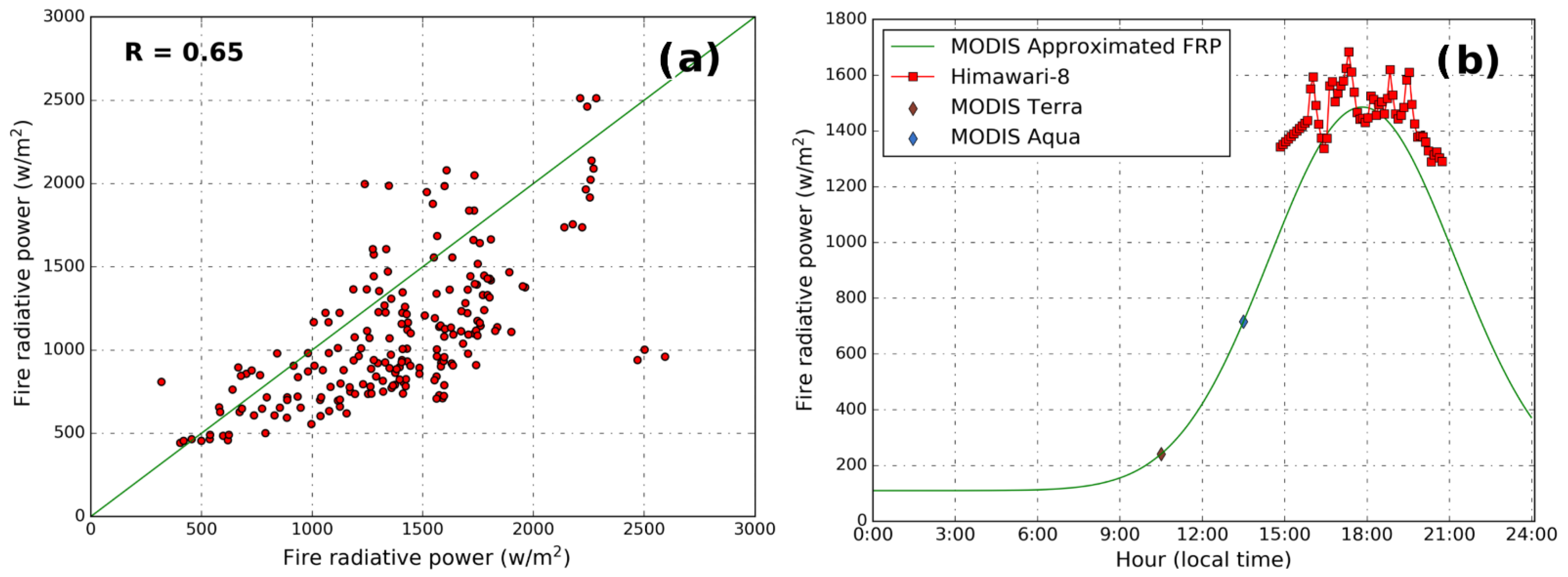
4.4.1. Validation with Himawari-8 FRP Data

FRP derived from Geosynchronous Earth Orbit satellite Himawari-8 was compared to the FRP derived from MODIS. Himawari-8 FRP data used in this study were derived from the level 2 brightness temperature product following the method introduced by Kim et al. [64] and Wooster et al. [65]. Figure 7a compares the peak FRP approximated by MODIS to Himawari-8 observations of FRP during the assumed peak burning hour (18:00 local time). Both datasets agreed well with each other, with Pearson correlation coefficient (R) of 0.65. Figure 7b shows an example of comparison of FRP between MODIS and Himawari-8. FRP derived from MODIS with the assumed diurnal cycle matched the Himawari-8 observations. The assumed diurnal cycle reproduced the peak value and the peak burning hours (≈6 p.m. local time) very well. The result indicates our method produced reliable and consistent FRP observations that can be used for emission approximation in this study.

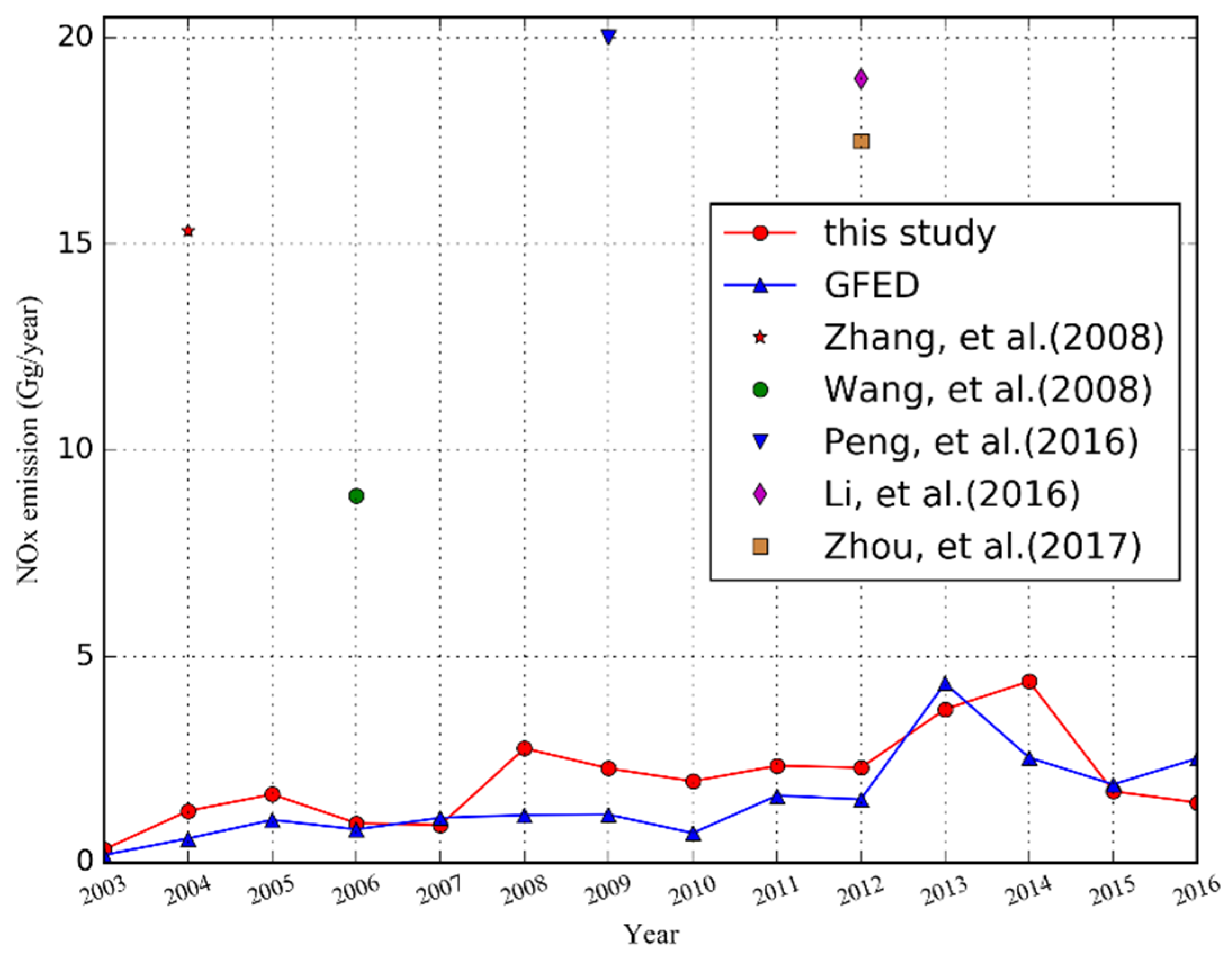
4.4.2. Comparison with Previous Studies and Existing Database

The Global Fire Emission Database provides comprehensive fire emission information [66]. The GFED 4.1s product used in the comparison has already taken small fires into account. As shown in Figure 8, our results are in the same order of magnitude as GFED from 2003 to 2016, with a correlation coefficient of 0.7 and RMSE (root mean square error) of 0.94 Gg/year. The NO_x emission of agricultural source biomass burning in Hubei generally showed an increasing trend from 2003 to 2014, followed by a decrease. This was partly related to the implementation of the policy on the ban of burning crop residues in 2014. Comparing NO_x emissions of our results to GFED, the lowest emission appeared in 2003 from both datasets. The peak emission of our results in 2014 was 4.40 Gg, while GFED showed the highest emission of 4.35 Gg in 2013.

Furthermore, we focused on comparing the spatial distribution of emission from the two datasets. We took the annual October as an example when crop residue burning was most vigorous. As our emission inventory was in a spatial resolution of 1 × 1 km, which is finer than the GFED database of 0.25° × 0.25°, we therefore gridded our dataset to the resolution of 0.25° × 0.25° for intercomparison (Figure 9d–f). As shown in Figure 9d,e,j,k, the spatial distribution of NO_x emissions from our results and GFED were consistent. The regions with higher emission were found at the junction of Xiaogan, Tianmen, and Xiantao, and the contiguous area of Jingzhou and Qianjiang, which covers a large portion of the cultivated land in the Jianghan Plain. The remaining part of NO_x emissions was sparsely scattered in Xiangyang, south of Huanggang, and central Jingmen at a low level. There was a slight difference in the two datasets in October 2016. Our results showed that the higher NO_x emissions were mainly observed in small parts of southern Xiaogan, Tianmen, Xiantao, and Jingzhou. However, GFED also showed higher emissions in northwest Xiaogan and eastern Wuhan in comparison with our result.

Although the NO_x emissions derived from this study were consistent with the GFED data in both temporal and spatial distribution, GFED was underestimated in most years due to the coarse resolution. However, in this study, the spatiotemporal resolution of MOD14A1/MYD14A1 (daily 1 × 1 km) products was much higher than that of the MCD64A1 product (monthly 0.25° × 0.25°) adopted in the GFED dataset. As a result, lower temporal resolution probably omitted the multiple occurrences of residue burning in small areas. Compared with the spatial resolution of 0.25°, 1 km resolution product of MOD14A1/MYD14A1 was more reliable in capturing small-scale and short-time burning. Moreover, this study took the phenological characteristics of different crops into consideration in order to further improve the accuracy of estimation. For example, the residue burning of corn and cotton contributed to 37% of NO_x emissions, which is much higher than that of rice and other kinds of crop types [6]. Meanwhile, we compared our results to previous studies [6,8,12,56,59]. As shown in Figure 8, NO_x emissions of residue burning derived in our study were considerably lower than that of Zhou et al. [55], Zhang et al. [8], Wang et al. [12], Peng et al. [58], and Li et al. [10]. Zhou et al. [55] calculated 17.5 Gg in 2012, which is approximately six times higher than our result of 2.31 Gg; Wu et al. [6] estimated total NO_x emissions of 173 Gg in Hubei from 2003 to 2015, which shows a relatively large difference from the 26.66 Gg estimated in this study. The methods they used were on the basis of the MODIS burned area product. The actual burned areas could span less than integrated MODIS pixels, covering only small fractions of each pixel in some conditions. Results from this for 2004, 2006, 2009, and 2012 were 1.26, 0.96, 2.29, and 2.31 Gg, respectively. Moreover, the NO_x emissions from residue burning in Hubei by Zhang et al. [8] in 2004 was 15.32 ± 0.92 Gg, Wang et al. [12] in 2006 found 8.9 Gg, Peng et al. [58] estimated the NO_x emission of 20 Gg in 2009, and Li et al. [10] found 19 Gg in 2012 (Figure 8). The methods they adopted were primarily based on the traditional bottom-up approaches, which were mostly optimized by adding auxiliary data and questionnaires. Their methods took regional differences between the proportion of open-field crop residue burning and EFs into consideration, but the incomplete statistical data may lead to uncertainties. Furthermore, in the previous studies, estimation of NO_x emissions from crop residue burning in some areas usually directly started from the trace of biomass consumption, which ignored the imperfect combustion, with the statistic biomass consumption tending to be much less than the actual biomass consumption. This study used FRP data, which provides a more reliable estimation of NO_x emissions from residue burning with consideration of crop phenology and an elaborate crop distribution map.

4.4.3. Comparison with Space-Based Observations

The spatial distribution of emissions estimated in this study was compared to NO₂ VCDs observed by the OMI sensor onboard the Aura platform. The NASA standard OMI NO₂ product version 3 [35] was used in this study. Tropospheric NO₂ VCDs were gridded onto a high resolution (0.01° × 0.01°) latitude–longitude grid following the approach described in Chan et al. [67,68,69]. In the regrinding process, we filtered data affected by the row abnormally issue of OMI and affected by cloud pixels with cloud radiance fraction larger than 0.5. The processed dataset was then further averaged to monthly means for analysis.

We compared the monthly average emission pattern to OMI observations of NO₂ columns. NO₂ VCDs derived from OMI were tropospheric columns that were affected by all kinds of emission sources, including industry, transportation, agriculture, and natural surface processes. The satellite measurements represent the NO₂ level as dispersion and reaction with other atmospheric species. In contrast, the dataset derived in this study was purely emission from agricultural-related burning. Therefore, these datasets cannot be compared directly. Instead, we looked into their spatiotemporal correlation. In order to separate the crop residue burning from other non-agricultural sources, we analyzed the differences in the spatial patterns observed in different seasons. As most of the burning processes are mainly concentrated in October after harvesting, we were able to separate the burning emission by taking the differences of NO₂ VCDs observed in September and October. As the other emissions might be considered approximately the same, the approach could eliminate the impacts from non-agricultural sources.

Our results were regridded to 0.1° × 0.1° to be more comparable to OMI observations (Figure 9a–c). Some NO₂ VCD peaks can be seen in southern Jingzhou and Jianghan Plain, which were related to crop residue burning. In October 2014, both our results (Figure 9a) and OMI VCDs (Figure 9g) showed a wide range of high NO_x emission/concentration in the Jianghan Plain, as well as in south Huanggang. In October 2015, our results obviously reflected the high NO_x emissions in central and southern Wuhan, as well as some sporadic abnormal emissions in Jingmen, Xiangfan, and Jingzhou (Figure 9b). OMI VCDs were consistent with our results in central and southern Wuhan, while the high NO₂ concentration was also observable at the edges of Wuhan, Huanggang, and Ezhou, which are dominated by non-agricultural emissions (Figure 9h). In order to eliminate the influence from other anthropogenic emissions, we looked at the difference of NO₂ VCDs between September (a month with much less burning activities) and October (a month with peak burning activities), as shown in Figure 9i,j. In October 2016, both results generally agreed with each other, especially in southern Wuhan and Tianmen (Figure 9c,i). Overall, our new emission database was in general consistent with OMI VCDs, especially in agricultural regions.

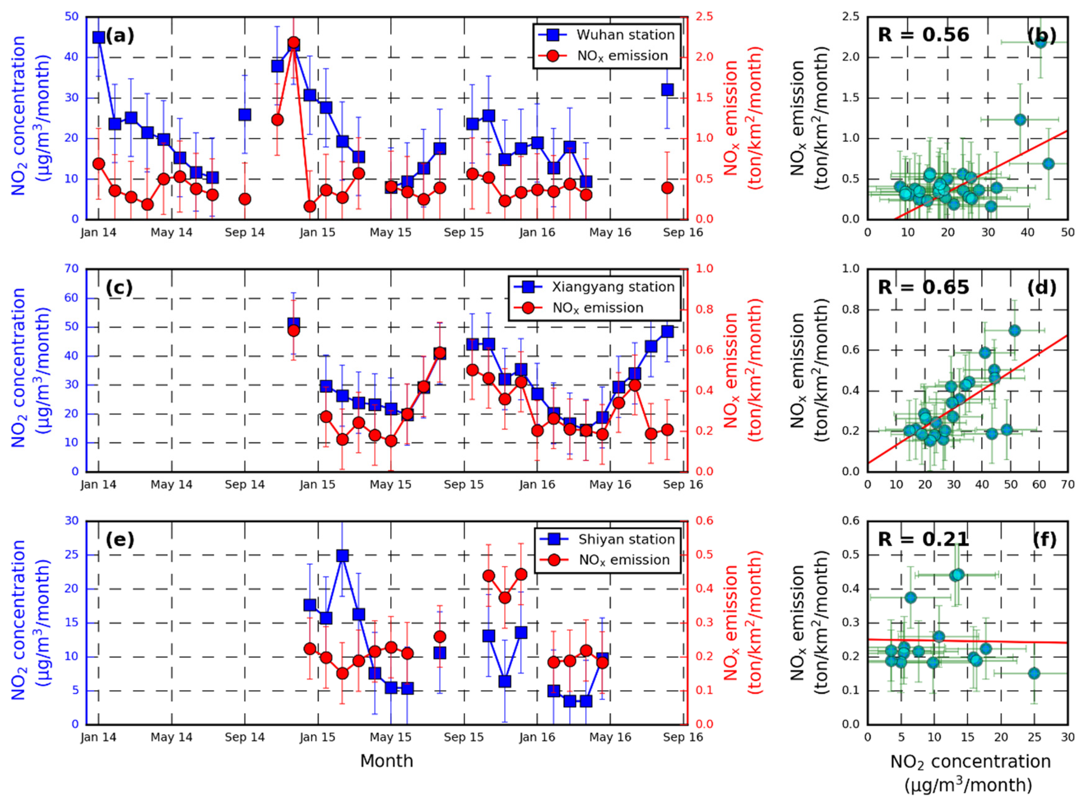
4.4.4. Comparison with In Situ Observations

We also compared our results to in situ observations derived from environmental monitoring stations. However, most of the environmental monitoring stations were in the urban areas where NO₂ is mainly emitted from non-agricultural pollution sources, e.g., traffic, power generation, and industrial emissions. In order to obtain the data that can accurately reflect the real situation of NO_x from residue burning, we adopted information from three rural environmental monitoring stations. These stations are in the southwest of Wuhan near the cropland, in the forest in southeast Shiyan, and in the suburbs near the cropland in southeast Xiangyang (Figure 1). It should be noted that the observations derived from a monitoring station located in Wuhan covered a time span from 2014 to 2016, while the other stations began to collect data until 2015, not providing a full coverage of the experiment period. In this study, we used the average NO_x emission calculated within 10 km of the monitoring stations to compare with the corresponding in situ NO₂ measurements. The NO₂ concentrations reported by the monitoring stations were not only related to the emission strength, but also strongly influenced by meteorological factors, other atmospheric chemistry processes, and sources other than crop residue burning. We compared the temporal variation trends between emission and in situ observations rather than a quantitative comparison of the absolute value.

Figure 10 shows the time series of NO_x emission estimated in this study and NO₂ concentrations observed by the three stations. The temporal variations of our results in all three stations were in general consistent with the NO_x concentrations observed by ground stations in Hubei from 2014 to 2016. Both data showed higher emissions/concentrations in autumn and winter, and low emissions/concentrations in spring and summer. The pattern was consistent with the temporal pattern of open-field crop residue burning in Hubei. The annual maximum emission/concentration in the months from October to February was likely due to the low boundary layer height and enhanced emissions related to higher power consumption in winter. Moreover, the stagnation of cold air and low precipitation in autumn and winter also reduced atmospheric transportation [50]. The lowest emission/concentration was observed in summer (June–August), as the abundant rainfall and monsoon combined with the higher photolysis rate significantly contribute to the shorter atmospheric lifetime [70]. Larger differences between our results and in situ observations were found in April of Shiyan and in November and December of Xiangyang (Figure 9b,c). The difference in April was likely related to frequent forest fires caused by the prevalence of sacrifice activities in spring, while in November and December, the difference was probably related to the pollution transport from urban to the suburban area. In addition, increased domestic heating and energy consumption in these months also enhanced the contribution from non-biomass burning emissions.

5. Conclusions

In this paper, we presented a new method to improve the estimation of agricultural-related burning NO_x emission. We applied this new method to estimate crop residue burning emission of NO_x from 2014 to 2016 in Hubei, China. The new database characterized burning emissions down to the field level by combining statistical data and satellite remote sensing measurements. The spatiotemporal resolution of the dataset was improved to a daily 1 × 1 km grid. The new emission database was evaluated by comparing to geostationary FRP product, OMI satellite observations, in situ monitoring station data, and the GFED emission database. The derived spatial distribution of NO_x emission agreed with the OMI observations of NO₂ vertical columns. The temporal variation of the NO_x emission also showed good consistency with geostationary satellite observations in the cases mentioned in Section 4.4.1 and in situ monitoring observations in the rural sites.

In addition, this database took field-level agricultural emission into consideration, which is theoretically more accurate for estimation of emission over regions with intricate cultivation structure, i.e., Hubei. The new emission database with an enhanced spatiotemporal resolution can potentially improve the regional chemistry transport model simulation of pollution transport and can provide support for the environmental protection agency when designing air quality-related policies.

References

1. Gao, C.; Zhang, C.; Yu, S. Temporal and spatial variation for vertical column density of tropospheric NO2 over the Yangtze River Delta from 2005 to 2013. J. Zhejiang A&F Univ. 2015, 32, 691–700. [Google Scholar]
2. Jang, M.; Kamens, R.M. Characterization of secondary aerosol from the photooxidation of toluene in the presence of NO x and 1-propene. Environ. Sci. Technol. 2001, 35, 3626–3639. [Google Scholar] [CrossRef] [PubMed]
3. Shepherd, M.F.; Barzetti, S.; Hastie, D.R. The production of atmospheric NOx and N2O from a fertilized agricultural soil. Atmos. Environ. Part A Gen. Top. 1991, 25, 1961–1969. [Google Scholar] [CrossRef]
4. Gao, J.; Zhu, B.; Wang, Y.; Kang, H. Distribution and long-term variation of troposphric NO2 over China during 2005 to 2013. China Environ. Sci. 2015, 35, 2307–2318. [Google Scholar]
5. Cao, Y.-s.; Tian, Y.; Yin, B.; Zhu, Z. Investigation on NO Emission from Agricultural Soils. Soils 2013, 45, 791–799. [Google Scholar]
6. Wu, J.; Kong, S.; Wu, F.; Cheng, Y.; Zheng, S.; Yan, Q.; Zheng, H.; Yang, G.; Zheng, M.; Liu, D. Estimating the open biomass burning emissions in central and eastern China from 2003 to 2015 based on satellite observation. Atmos. Chem. Phys. 2018, 18, 11623–11646. [Google Scholar] [CrossRef] [Green Version]
7. Xin, H.; Li, M.; Li, J.; Yu, S. A high-resolution emission inventory of crop burning in fields in China based on MODIS Thermal Anomalies/Fire products. Atmos. Environ. 2012, 50, 9–15. [Google Scholar]
8. Zhang, H.; Ye, X.; Cheng, T.; Chen, J.; Yang, X.; Wang, L.; Zhang, R. A laboratory study of agricultural crop residue combustion in China: Emission factors and emission inventory. Atmos. Environ. 2008, 42, 8432–8441. [Google Scholar] [CrossRef]
9. Liu, M.; Song, Y.; Yao, H.; Kang, Y.; Li, M.; Huang, X.; Hu, M. Estimating emissions from agricultural fires in the North China Plain based on MODIS fire radiative power. Atmos. Environ. 2015, 112, 326–334. [Google Scholar] [CrossRef]
10. Li, J.; Bo, Y.; Xie, S. Estimating emissions from crop residue open burning in China based on statistics and MODIS fire products. J. Environ. Sci. 2016, 44, 158–170. [Google Scholar] [CrossRef] [Green Version]
11. Li, J.; Li, Y.; Bo, Y.; Xie, S. High-resolution historical emission inventories of crop residue burning in fields in China for the period 1990–2013. Atmos. Environ. 2016, 138, 152–161. [Google Scholar] [CrossRef]
12. Wang, S.; Zhang, C. Spatial and temporal distribution of air pollutant emissions from open burning of crop residues in China. Sci. Technol. Mag. Online 2008, 3, 329–333. [Google Scholar]
13. Qiu, X.; Duan, L.; Chai, F.; Wang, S.; Yu, Q.; Wang, S. Deriving High-Resolution Emission Inventory of Open Biomass Burning in China based on Satellite Observations. Environ. Sci. Technol. 2016, 50, 11779–11786. [Google Scholar] [CrossRef]
14. Randerson, J.; Chen, Y.; Van Der Werf, G.; Rogers, B.; Morton, D. Global burned area and biomass burning emissions from small fires. J. Geophys. Res. Biogeosci. 2012, 117. [Google Scholar] [CrossRef]
15. Andela, N.; Van, d.W.; Guido, R.; Kaiser, J.W.; Van Leeuwen, T.T.; Wooster, M.J.; Lehmann, C.E.R. Biomass burning fuel consumption dynamics in the tropics and subtropics assessed from satellite. Biogeosciences 2016, 13, 1–30. [Google Scholar]
16. Ellicott, E.; Vermote, E.; Giglio, L.; Roberts, G. Estimating biomass consumed from fire using MODIS FRE. Geophys. Res. Lett. 2009, 36, 401–405. [Google Scholar] [CrossRef] [Green Version]
17. Yin, L.; Du, P.; Zhang, M.; Liu, M.; Xu, T.; Song, Y. Estimation of emissions from biomass burning in China (2003–2017) based on MODIS fire radiative energy data. Biogeosciences 2019, 16, 1629–1640. [Google Scholar] [CrossRef] [Green Version]
18. Wooster, M.J.; Roberts, G.; Perry, G.; Kaufman, Y. Retrieval of biomass combustion rates and totals from fire radiative power observations: FRP derivation and calibration relationships between biomass consumption and fire radiative energy release. J. Geophys. Res. Atmos. 2005, 110, 311–330. [Google Scholar] [CrossRef]
19. Seiler, W.; Crutzen, P.J. Estimates of gross and net fluxes of carbon between the biosphere and the atmosphere from biomass burning. Clim. Chang. 1980, 2, 207–247. [Google Scholar] [CrossRef]
20. Badarinath, K.; Chand, T.; Prasad, V.K. Agriculture crop residue burning in the Indo-Gangetic Plains--A study using IRS-P6 AWiFS satellite data. Curr. Sci. 2006, 91, 1085–1089. [Google Scholar]
21. Xing, X.; Zhou, Y.; Lang, J.; Chen, D.; Cheng, S.; Han, L.; Huang, D.; Zhang, Y. Spatiotemporal variation of domestic biomass burning emissions in rural China based on a new estimation of fuel consumption. Sci. Total Environ. 2018, 626, 274–286. [Google Scholar] [CrossRef]
22. Lin, H.W.; Jin, Y.; Giglio, L.; Foley, J.A.; Randerson, J.T. Evaluating greenhouse gas emissions inventories for agricultural burning using satellite observations of active fires. Ecol. Appl. 2012, 22, 1345–1364. [Google Scholar] [CrossRef]
23. Yu, C.; Chen, L.-F.; LI, S.-S.; Tao, J.-H.; Su, L. Estimating Biomass Burned Areas from Multispectral Dataset Detected by Multiple-Satellite. Spectrosc. Spectr. Anal. 2015, 35, 739–745. [Google Scholar]
24. Palumbo, I.; Grégoire, J.; Boschetti, L.; Eva, H. Fire regimes in protected areas of sub-saharan Africa, derived from the GBA2000 dataset. In Proceedings of the Innovative Concepts and Methods in Fire Danger Estimation, 4th Workshop on Remote Sensing and GIS Applications to Forest Fire Management, EARSEL, Ghent, Belgium, 5–7 June 2003. [Google Scholar]
25. Kaufman, Y.J.; Justice, C.O.; Flynn, L.P.; Kendall, J.D.; Prins, E.M.; Giglio, L.; Ward, D.E.; Menzel, W.P.; Setzer, A.W. Potential global fire monitoring from EOS-MODIS. J. Geophys. Res. Atmos. 1998, 103, 32215–32238. [Google Scholar] [CrossRef]
26. Fornacca, D.; Ren, G.; Xiao, W. Performance of Three MODIS Fire Products (MCD45A1, MCD64A1, MCD14ML), and ESA Fire_CCI in a Mountainous Area of Northwest Yunnan, China, Characterized by Frequent Small Fires. Remote Sens. 2017, 9, 1131. [Google Scholar]
27. Cao, G.; Zhang, X.; Wang, D.; Zheng, F. Inventory of atmospheric pollutants discharged from biomass burning in China continent. China Environ. Sci. 2005, 25, 389–393. [Google Scholar]
28. Bing, L.U.; Fei, K.S.; Han, B.; Yan, W.X.; Peng, B.Z. Inventory of atmospheric pollutants discharged from biomass burning in China continent in 2007. China Environ. Sci. 2011, 31, 186–194. [Google Scholar]
29. Zhou, Y. Establishment of a high-resolution emission inventory and its evaluation through air quality for Jiangsu Province, China. Master’s Thesis, Nanjing University, Nanjing, China, 2016. [Google Scholar]
30. Streets, D.G.; Yarber, K.F.; Woo, J.H.; Carmichael, G.R. Biomass burning in Asia: Annual and seasonal estimates and atmospheric emissions. Glob. Biogeochem. Cycles 2003, 17, 1–20. [Google Scholar] [CrossRef] [Green Version]
31. Giglio, L.; Justice, C. MOD14A1 MODIS/Terra Thermal Anomalies/Fire Daily L3 Global 1 km SIN Grid V006 [Data set]; EOSDIS Land Processes DAAC: Sioux Falls, SD, USA, 2015. [CrossRef]
32. Giglio, L. MOD14A1 v006. Available online: https://lpdaac.usgs.gov/products/mod14a1v006/ (accessed on 8 February 2000).
33. Liu, X.; Zhai, H.; Shen, Y.; Lou, B.; Jiang, C.; Li, T.; Hussain, S.B.; Shen, G. Large Scale Crop Mapping from Multi-Source Remote Sensing Images in Google Earth Engine. IEEE J. Sel. Top. Appl. Earth Obs. Remote Sens. 2020. [Google Scholar] [CrossRef]
34. Levelt, P.F.; Hilsenrath, E.; Leppelmeier, G.W.; van den Oord, G.H.; Bhartia, P.K.; Tamminen, J.; de Haan, J.F.; Veefkind, J.P. Science objectives of the ozone monitoring instrument. IEEE Trans. Geosci. Remote Sens. 2006, 44, 1199–1208. [Google Scholar] [CrossRef]
35. Chan, K.L.; Wang, Z.; Ding, A.; Heue, K.-P.; Shen, Y.; Wang, J.; Zhang, F.; Shi, Y.; Hao, N.; Wenig, M. MAX-DOAS measurements of tropospheric NO2 and HCHO in Nanjing and a comparison to ozone monitoring instrument observations. Atmos. Chem. Phys. 2019, 19. [Google Scholar] [CrossRef] [Green Version]
36. Krotkov, N.A.; Lamsal, L.N.; Celarier, E.A.; Swartz, W.H.; Marchenko, S.V.; Bucsela, E.J.; Chan, K.L.; Wenig, M.; Zara, M. The version 3 OMI NO2 standard product. Atmos. Meas. Tech. 2017, 10, 3133–3149. [Google Scholar] [CrossRef] [Green Version]
37. González Abad, G.; Liu, X.; Chance, K.; Wang, H.; Kurosu, T.P.; Suleiman, R. Updated Smithsonian Astrophysical Observatory Ozone Monitoring Instrument (SAO OMI) formaldehyde retrieval. Atmos. Meas. Tech. 2015, 8, 19–32. [Google Scholar] [CrossRef] [Green Version]
38. Marchenko, S.; Krotkov, N.A.; Lamsal, L.N.; Celarier, E.A.; Swartz, W.H.; Bucsela, E.J. Revising the slant column density retrieval of nitrogen dioxide observed by the Ozone Monitoring Instrument: REVISED NO 2 RETRIEVAL FOR OMI. J. Geophys. Res. Atmos. 2015, 120. [Google Scholar] [CrossRef] [Green Version]
39. Solomon, S.; Schmeltekopf, A.L.; Sanders, R.W. On the interpretation of zenith sky absorption measurements. J. Geophys. Res. Atmos. 1987, 92, 8311–8319. [Google Scholar] [CrossRef]
40. Rotman, D.A.; Tannahill, J.R.; Kinnison, D.E.; Connell, P.S.; Bergmann, D.; Proctor, D.; Rodriguez, J.M.; Lin, S.J.; Rood, R.B.; Prather, M.J.; et al. Global Modeling Initiative assessment model: Model description, integration, and testing of the transport shell. J. Geophys. Res. Atmos. 2001, 106, 1669–1691. [Google Scholar] [CrossRef] [Green Version]
41. Xu, W.; Wooster, M.J.; Kaneko, T.; He, J.; Zhang, T.; Fisher, D. Major advances in geostationary fire radiative power (FRP) retrieval over Asia and Australia stemming from use of Himarawi-8 AHI. Remote Sens. Environ. 2017, 193, 138–149. [Google Scholar] [CrossRef] [Green Version]
42. Vermote, E.; Ellicott, E.; Dubovik, O.; Lapyonok, T.; Chin, M.; Giglio, L.; Roberts, G.J. An approach to estimate global biomass burning emissions of organic and black carbon from MODIS fire radiative power. J. Geophys. Res. Atmos. 2009, 114. [Google Scholar] [CrossRef]
43. Vadrevu, K.P.; Csiszar, I.; Ellicott, E.; Giglio, L.; Badarinath, K.V.S.; Vermote, E.; Justice, C. Hotspot Analysis of Vegetation Fires and Intensity in the Indian Region. IEEE J. Sel. Top. Appl. Earth Obs. Remote Sens. 2013, 6, 224–238. [Google Scholar] [CrossRef]
44. Wu, J.; Kong, S.; Wu, F.; Cheng, Y.; Zheng, S.; Qin, S.; Liu, X.; Yan, Q.; Zheng, H.; Zheng, M. The moving of high emission for biomass burning in China: View from multi-year emission estimation and human-driven forces. Environ. Int. 2020, 142, 105812. [Google Scholar] [CrossRef]
45. Xi-bin, T.; Cheng, H.; Sheng-rong, L.; Li-ping, Q.; Hong-li, W.; Min, Z.; Ming-hua, C.; Chang-hong, C.; Qian, W.; Gui-ling, L.I.; et al. Emission Factors and PM Chemical Composition Study of Biomass Burning in the Yangtze River Delta Region. Environ. Sci. Technol. 2014, 35, 1623–1632. [Google Scholar]
46. Min, H.; Xing-rui, W.; Li, H.; Xiao-qiong, F.; Xue, M. Emission Inventory of Crop Residues Field Burning and Its Temporal and Spatial Distribution in Sichuan Province. Environ. Sci. Technol. 2015, 4, 1208–1216. [Google Scholar]
47. Guan, Y.; Chen, G.; Cheng, Z.; Yan, B.; Hou, L.A. Air pollutant emissions from straw open burning: A case study in Tianjin. Atmos. Environ. 2017, 171, 155–164. [Google Scholar] [CrossRef]
48. National Bureau of Statistics. Available online: http://www.stats.gov.cn/tjsj/ndsj/ (accessed on 25 October 2005).
49. Cao, G.; Zhang, X.; Gong, S.; Zheng, F. Investigation on emission factors of particulate matter and gaseous pollutants from crop residue burning. J. Environ. Sci. 2008, 20, 50–55. [Google Scholar] [CrossRef]
50. Li, X.; Wang, S.; Duan, L.; Hao, J.; Li, C.; Chen, Y.; Yang, L. Particulate and trace gas emissions from open burning of wheat straw and corn stover in China. Environ. Sci. Technol. 2007, 41, 6052–6058. [Google Scholar] [CrossRef]
51. Zhang, J.; Smith, K.R.; Ma, Y.; Ye, S.; Jiang, F.; Qi, W.; Liu, P.; Khalil, M.A.K.; Rasmussen, R.A.; Thorneloe, S.A. Greenhouse gases and other airborne pollutants from household stoves in China: A database for emission factors. Atmos. Environ. 2000, 34, 4537–4549. [Google Scholar] [CrossRef] [Green Version]
52. Zhang, Y.; Shao, M.; Lin, Y.; Luan, S.; Mao, N.; Chen, W.; Wang, M. Emission inventory of carbonaceous pollutants from biomass burning in the Pearl River Delta Region, China. Atmos. Environ. 2013, 76, 189–199. [Google Scholar] [CrossRef]
53. Li, J.; Song, Y.; Li, M.; Huang, X. Estimating Air Pollutants Emissions from Open Burning of Crop Residues in Jianghan Plain. Acta Sci. Nat. Univ. Pekin. 2015, 51, 647–656. [Google Scholar]
54. Freeborn, P.H.; Wooster, M.J.; Roberts, G. Addressing the spatiotemporal sampling design of MODIS to provide estimates of the fire radiative energy emitted from Africa. Remote Sens. Environ. 2011, 115, 475–489. [Google Scholar] [CrossRef]
55. Zhou, Y.; Xing, X.; Lang, J.; Chen, D.; Cheng, S.; Lin, W.; Xiao, W.; Liu, C. A comprehensive biomass burning emission inventory with high spatial and temporal resolution in China. Atmos. Chem. Phys. 2017, 17, 2839–2864. [Google Scholar] [CrossRef] [Green Version]
56. Rabin, S.S.; Magi, B.; Shevliakova, E.; Pacala, S.W. Quantifying regional, time-varying effects of cropland and pasture on vegetation fire. Biogeosciences 2015, 12, 6591–6604. [Google Scholar] [CrossRef] [Green Version]
57. Kumar, V.; Sarkar, C.; Sinha, V. Influence of post-harvest crop residue fires on surface ozone mixing ratios in the NW IGP analyzed using 2 years of continuous in situ trace gas measurements. J. Geophys. Res. Atmos. 2016, 121, 3619–3633. [Google Scholar] [CrossRef] [Green Version]
58. Peng, L.; Zhang, Q.; He, K. Emission inventory of atmospheric pollutants from open burning of crop residues in China based on a national questionnaire. Res. Environ. Sci. 2016, 29, 1109–1118. [Google Scholar]
59. Liu, Z.; Xu, A.; Long, B. Energy from combustion of rice straw: Status and challenges to China. Energy Power Eng. 2011, 3, 325–331. [Google Scholar] [CrossRef] [Green Version]
60. Peng, J. Research status and prospect of rape straw utilization. Rural Sci. Technol. 2016, 38, 26. [Google Scholar]
61. Preliminary Evaluation of Agricultural Surface Quadrats and Remote Sensing Monitoring in Hubei Province from 2015 to 2017; Agricultural Remote Sensing Application Center Wuhan. Available online: http://zhxy.hubu.edu.cn/info/1386/5141.htm (accessed on 2 December 2009).
62. He, Q.; Liu, C. Improved Algrithom of Self-adaptive Fire detection for MODIS Data. J. Remote Sens. 2008, 12, 448–453. [Google Scholar]
63. Wang, K.; Zhang, J. Extraction of rape seed cropping distribution information in Hubei Province based on MODIS images. Remote Sens. Territ. Resour. 2015, 27, 65–70. [Google Scholar]
64. Kim, D.; Cho, J.; Hong, S.; Lee, H.; Won, M.; Byun, S.; Park, K.; Lee, Y.-W. First retrieval of fire radiative power from COMS data using the mid-infrared radiance method. Remote Sens. Lett. 2017, 8, 116–125. [Google Scholar] [CrossRef]
65. Wooster, M.; Zhukov, B.; Oertel, D. Fire radiative energy for quantitative study of biomass burning: Derivation from the BIRD experimental satellite and comparison to MODIS fire products. Remote Sens. Environ. 2003, 86, 83–107. [Google Scholar] [CrossRef]
66. Randerson, J.T.; Van Der Werf, G.R.; Giglio, L.; Collatz, G.J.; Kasibhatla, P.S. Global Fire Emissions Database, Version 4.1 (GFEDv4); ORNL Distributed Active Archive Center: Oak Ridge, TN, USA, 2017. [CrossRef]
67. Chan, K.L.; Wiegner, M.; Wenig, M.; Pöhler, D. Observations of tropospheric aerosols and NO2 in Hong Kong over 5 years using ground based MAX-DOAS. Sci. Total Environ. 2018, 619, 1545–1556. [Google Scholar] [CrossRef]
68. Chan, K.L.; Pöhler, D.; Kuhlmann, G.; Hartl, A.; Platt, U.; Wenig, M.O. NO2 measurements in Hong Kong using LED based long path differential optical absorption spectroscopy. Atmos. Meas. Tech. 2012, 5, 901–912. [Google Scholar] [CrossRef] [Green Version]
69. Chan, K.L.; Hartl, A.; Lam, Y.; Xie, P.; Liu, W.; Cheung, H.; Lampel, J.; Pöhler, D.; Li, A.; Xu, J. Observations of tropospheric NO2 using ground based MAX-DOAS and OMI measurements during the Shanghai World Expo 2010. Atmos. Environ. 2015, 119, 45–58. [Google Scholar] [CrossRef]
70. Wang, Y.; Zhang, Y.; Hao, J.; Luo, M. Seasonal and spatial variability of surface ozone over China: Contributions from background and domestic pollution. Atmos. Chem. Phys. 2011, 11, 3511–3525. [Google Scholar] [CrossRef] [Green Version]
Figure 1. Study area and positions of the environmental monitoring station.
Remotesensing 13 00404 g001
Figure 2. Time series of daily and monthly fire count (per day) detected by MODIS over Hubei from 2014 to 2016. The fire counts are separated into the four land cover types.
Remotesensing 13 00404 g002
Figure 3. Fire distribution maps for different crop types during 2014–2016: (a) rice, (b) corn and cotton, (c) rapeseed and wheat, and (d) non-cultivated land.
Remotesensing 13 00404 g003
Figure 4. Time series of daily maximum fire radiative power (FRP) for four land covers for the period 2014–2016: (a) rice, (b) corn and cotton, (c) rapeseed and wheat, and (d) non-cultivated land.
Remotesensing 13 00404 g004
Figure 5. NOx emissions of crop residue burning from different land covers in Hubei during 2014–2016.
Remotesensing 13 00404 g005
Figure 6. Spatial distribution of accumulated NOx emissions from 2014 to 2016 for different land covers: (a) rice, (b) corn and cotton, (c) rapeseed and wheat, (d) non-cultivated land.
Remotesensing 13 00404 g006
Figure 7. Evaluations of FRP between Himawari-8 and moderate resolution imaging spectroradiometer (MODIS) observations with assumed diurnal cycle: (a) scatter plot of Himawari-8 measurements and FRPs approximated from MODIS, (b) comparison of FRP between Himawari-8 observations and assumed diurnal cycle from MODIS.
Remotesensing 13 00404 g007
Figure 8. Comparison of crop residue burning emission of NOx derived in this study to the global fire emission database (GFED) database and previous studies.
Remotesensing 13 00404 g008
Figure 9. Spatial distribution of crop residue burning emissions of NOx by this study, GFED emission database and ozone monitoring instrument (OMI) tropospheric NO2 vertical column density, and our results. (ac) Our results on a 0.1° × 0.1° grid in October of 2014, 2015, and 2016, respectively. (df) Our results on a 0.25° × 0.25° grid in October of 2014, 2015, and 2016, respectively. (gi) The difference of OMI tropospheric NO2 vertical column densities (VCDs) between October and September in 2014, 2015, and 2016, respectively. (jl) The NOx emission from GFED database in October of 2014, 2015, and 2016, respectively.
Remotesensing 13 00404 g009
Figure 10. Time series of monthly crop residue burning NOx emission and in-situ measurements of NO2 concentrations of (a) Wuhan, (c) Xiangfan, and (e) Shiyan. (b,d,f), show the corresponding scatter plots for Wuhan, Xiangfan and Shiyan. Note that the emission data did not reflect any atmospheric process.
Remotesensing 13 00404 g010