Abstract
Capturing the spatial heterogeneity and characteristic scale is the key to determining the spatial patterns of land surfaces. In this research, the core observation area of the middle reaches of the Heihe River Basin was selected as the study area, and the scale identification of several typical objects was carried out by implementing experiments on moderate- and high-resolution remotely sensed ASTER and CASI NDVI images. The aim was to evaluate the potential of the local variance and semivariance analysis to characterize the spatial heterogeneity of objects, track their changes with scale, and obtain their scales. Our results show that natural objects have multiscale structures. For a single object with a recognizable size, the results of the two methods are relatively consistent. For continuously distributed samples of indistinctive size, the scale obtained by the local variance is smaller than that obtained by the semivariance. As the image resolution becomes coarser and the research scopes expand, the scales of objects are also increasing. This article also indicates that with a small research area of uniform objects, the local variance and semivariance are easy to facilitate researchers to quickly select the appropriate spatial resolution of remote sensing data according to the research area.
1. Introduction
Spatial patterns are a significant geometric feature of terrestrial ecosystems and control the ecological process and function of the Earth’s surface [1]. They have been widely used in various studies in the fields of ecology and geoscience [2,3,4]. With the rapid development of space technology in the 20th century, a series of satellites integrating different types of sensors have been successively launched by different nations, boosting earth observations on a large scale and providing sufficient spatiotemporal data sources for geographical research [5]. In particular, high-spatial-resolution satellite images can significantly improve the capacity to capture and extract the spatial pattern information of the land surface.
In the domain of landscape ecology, the spatial pattern of ground objects is closely correlated with the observation scale [6]. Scale problems have been studied in a wide range of subjects [7,8,9,10]. In this research, the scale adopts the definition of “grain” in ecology, that is, the size of the spatial sampling cells used in exploration of spatial patterns [11,12,13]. It corresponds to the spatial resolution of remote sensing images. The properties or laws of objects obtained at one resolution may not be applicable at another resolution [14]. Some models of remote sensing inversion parameters have nonlinear characteristics. When nonlinear models are applied to parameter inversion on pixels with spatial heterogeneity, there is a certain deviation between the results and the real values [15]. The choice of a spatial resolution depends on several factors. They contain the information of objects, the analysis methods to be used to extract the information, and the spatial structure of the scene itself. Only by selecting remote sensing data with appropriate spatial resolution can the distribution of ground objects be accurately obtained. As the research moves along, the scale of the existing data cannot meet the actual application need. One solution is to decompose the pixels to an appropriate scale (the size of the pixels) by using spatial heterogeneity and scale analysis so that the inversion at this scale is unbiased and scale conversion is required [16,17]. Therefore, it is important to determine the appropriate scale for conversion. The appropriate scale, which is also known as the characteristic scale, is equivalent to the resolution of the image with the coarsest resolution that can identify the smallest and distinguishable ground objects in the image [18,19]. There may be multiple levels of objects in the scene. What we identify is the lowest level, that is, the smallest feature. For an object of a specific size, the characteristic scale is its size. The root of the scale lies in the spatial heterogeneity of the land surface. Li et al. contended that spatial heterogeneity refers to the degree of complexity or variability of the system characteristics in space [20], which is often manifested as the patchiness of an ecosystem and the multi-hierarchical structure of ground objects. Heterogeneity, in turn, has strong scale dependence [21]. Under coarse spatial resolutions, processes are considered to be homogeneous, but when increasing to a finer spatial resolution, they are considered heterogeneous. Therefore, heterogeneity is the key to comprehending the scale problem. Interior objects at different scales have diverse distribution rules, which reflect the multi-hierarchical structures of natural objects [22,23]. Taking forestland as an example, the object scale can be a leaf, a limb, a tree, or stands of trees. By comparing the characteristic changes in the same object at different scales, the spatial pattern of the surface can be fully grasped. In addition, as the scale attribute of the data does not change continuously, and due to the errors in the image and the analysis process, the obtained scale can only be a rough numerical range. Generally, researchers selected remote sensing data of a particular spatial resolution on the basis of what resolution is available from the different sensors or the practice and intuition of individuals. Therefore, they are very constricted in the choice of data resolution, and cannot choose certain resolution data according to their own actual needs. We are eager to obtain the spatial resolution of remote sensing images that can explore the distribution law of geographical objects. However, if the scale can be identified by analyzing the heterogeneity to automatically select the appropriate resolution images, it can not only reduce the uncertainty of data selection, but also improve the precision and accuracy of the information extracted. The contribution of our paper is to determine what resolution spatial data are suitable for scale conversion for a certain research object.
Remote sensing technology can effectively detect the spatial structure of ground objects, such as land cover changes [24], water pollution monitoring [25], and vegetation growth [26]. Remote sensing data for vegetation structure are currently provided at moderate spatial resolution, ranging from several hundred meters to one or a few kilometers. However, at such moderate resolution, the landscape is a mosaic of objects, such as cropland or vegetation patches, often smaller than moderate resolution pixels. The intrapixel spatial heterogeneity information will be lost. Therefore, if remote sensing data with higher spatial resolution can be obtained, the spatial heterogeneity of fine ground objects can be identified. Among the various inversion indices, the normalized differential vegetation index (NDVI) can reflect the growth status and physical and chemical properties of vegetation and is correlated with the leaf area index, vegetation coverage, and light utilization rate. [27]. The NDVI is considered the most robust variable for describing the heterogeneity of landscape ecosystems [28]. This parameter has been applied in numerous analyses of surface heterogeneity and multiscale exploration because of its simple inversion and close relationship to land cover changes [29,30]. Using high-resolution remote sensing images to study the heterogeneity and to identify the scale of the NDVI of fine objects in a study area is of great importance for agricultural production, planting structure determination, ecological environment assessment, and effective water resource utilization.
Heterogeneity emphasizes the nonuniformity of features in space and probes the spatial variation trend and autocorrelation characteristics of variables [31]. Scholars have conducted much research on how to quantitatively describe the spatial heterogeneity of surface objects and how to obtain the scale [20,32,33]. Sugihara et al. proposed the fractal dimension method [34]. When the resolution and research range of an image are changed, the time-division dimension becomes disordered, which makes it hard to extract the scale. The porosity index method proposed by Atkinson et al. is a landscape index method that is applicable to data of categorical variables, rather than numerical variables [35]. Ming et al. suggested an improved local variance method based on a variable window and variable resolution on the basis of predecessors [36]. Han et al. studied the scale of remote sensing classification based on the information entropy method [37]. The mean is constricted by the number of sample lines in the observation area and the layout direction, so the scale analysis of the overall image is slightly weak. The local variance method proposed by Woodcock et al. [38] and the semivariance method proposed by Webster et al. [39] are the two most widely used methods for analyzing spatial heterogeneity. They have similar mechanisms for the detection of spatial patterns by establishing the relationship between ground object sizes and the spatial resolution. In the current methods, the local variance and semivariance methods are simple and effective spatial statistics methods that can be applied to analyze spatially continuous quantitative data [40]. Many studies using these two methods only chose samples of a single sampling range or images with a single original spatial resolution, and only a single scale can be obtained [41,42,43]. However, features in nature have multiple hierarchical structures corresponding to multiple characteristic scales. If parts of the research gap can be filled, the application prospects of the two methods will be expanded. Additionally, until recently, it was found that most research in the heterogeneity field was aimed at solving the scale analysis of large-scale images to select the best spatial resolution [44,45]. Obviously, there are limitations to using a single scale to represent a complicated surface. At present, there are few studies on the spatial heterogeneity analysis and scale extraction of fine features. This research can fill in the knowledge gap regarding the scale of uniform ground objects in small-scope areas. In our research, two types of remote sensing data with different resolutions were used to explore the spatial distribution of the same ground objects with different sample sizes or research scopes (300 m × 300 m and 600 m × 600 m), and we wanted to observe how the two heterogeneous methods identified the scale of ground objects and the experimental results in the process of scale rising. Our research can identify and compare the scales of different objects. More importantly, different scales of the same object can be captured, which provides support for the exploration of continuous changes of the object scale. In this study, based on high-resolution satellite data and land cover data, local variance and semivariance analyses were applied to study the spatial heterogeneity and scale extraction of the NDVI of the fine features in the core observation area of the middle reaches of the Heihe River Basin (HRB). The study area and data preprocessing are detailed in Section 2. Then, the methods are presented in Section 3, followed by the results and discussion. The conclusions of this study are summarized at the end.
2. Materials and Preprocessing
2.1. Study Area and Data
The HRB is one of the second-largest inland basins in China, and is located in the arid zone of the northwestern part, and the Heihe River flows through three provinces: Gansu, Qinghai, and Inner Mongolia. The HRB ranges between 37.7°N–42.7°N and 97.1°E–102.0°E, with a drainage area of approximately 140,000 km2 [46]. The study focuses on the core observation area in the middle reaches of the basin within 30 × 30 km. The prefecture belongs to a typical temperate continental climate. Its territory is flat, and the maximum elevation difference is approximately 50 m. The crop planting block is broken, and the planting structure is complex [47]. It is a unique desert oasis with artificial irrigation agriculture regions farming wheat, corn, rice, beans, oil crops, and fruits and vegetables. Exploring the spatial pattern of oasis features plays an important role in coordinating the relationship between people and land and improving economic development.
Over the past three decades, a comprehensive watershed observation system has been implemented in this region. The National Natural Science Foundation of China research project "Integrated research on the ecohydrological process of the Heihe River Basin" was carried out. To exhibit and share the ground-based observations and remotely sensed products of the research, the Cold and Arid Regions Scientific Data Center was established. The data are now stored in the National Tibetan Plateau Third Pole Environment Data Center (http://data.tpdc.ac.cn/en/) for users to apply and access freely. The core area was selected to obtain a comprehensive understanding of the types and spatial distribution of the main ground objects. Its location and land use data of the study area are shown in Figure 1.
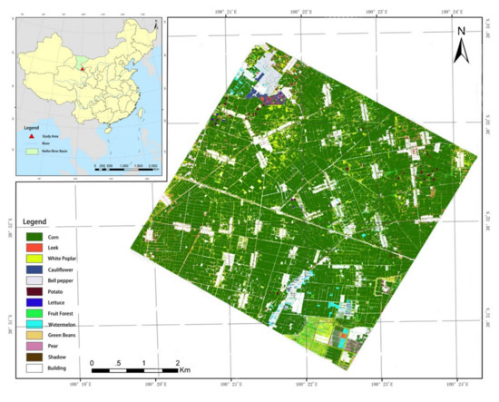
Figure 1.
The map of the study area.
Remote sensing band image data from the Compact Airborne Spectrographic Imager (CASI) and Advanced Spaceborne Thermal Emission and Reflection Radiometer (ASTER) and high-spatial resolution land use data were used in this study. The CASI data and land use data were collected from the data center, as mentioned above. The CASI visible/near-infrared data, totaling 48 bands, were obtained on 7 July 2012, and their spatial resolution was 1 m. Moreover, its spectral range is from 380 nm to 1050 nm, with a spectral resolution of 7.2 nm [48]. The ASTER image from 10 July 2012 was downloaded from the NASA website (https://worldwind.arc.nasa.gov/). It consists of three visible and near-infrared bands, six shortwave infrared bands, and five thermal infrared bands. However, only the visible and near-infrared bands with 15 m spatial resolution were actually used. The central wavelengths of the ASTER visible and near-infrared bands (Bands 1, 2, and 3N) are 556.1 nm, 661.0 nm, and 807.0 nm, respectively. The product level is L1 A data without atmospheric and geometric correction. The fine land use data used in this study involve clipped strips from land use products in the middle observation of the HRB. The land use products were retrieved by a hierarchical classification from CASI band images, with a total accuracy of 84.6%, and a kappa coefficient of 0.8262 [46,49]. Additionally, all the land use types in the study as the foci experimental area were investigated in the field experiment. Crops, woodland, and buildings are the main land use types in the area. The unclassified land type is the synthesis of all situations that do not belong to any specific land class. Unfortunately, other crop types are often mixed with them. The statistics on the area of each land use type are shown in Table 1. There are 13 types of land use except unclassified land.

Table 1.
Statistical table of the different land use areas in the core observation area.
2.2. Data Preprocessing
Prior to heterogeneity and scale analysis, the raw data needed to be preprocessed. For CASI data, the images were first geometrically corrected by the real-time kinematic (RTK) ground measured points. Then, radiometric and 6S atmospheric corrections were also performed on the raw band images to obtain corresponding land surface reflectance products. The ASTER image was radiometrically calibrated, and then the fast line-of-sight atmospheric analysis of spectral hypercubes (FLAASH) algorithm in ENVI 5.3 software was selected to implement the atmospheric correction. To resolve the geolocation error of the ASTER images, fine geometric correction was carried out based on the CASI image.
Following image preprocessing, the NDVI was inverted from two remote sensing datasets, which is a key index to describe vegetation spectral properties and is simple to calculate via only the red and near-infrared bands. The ASTER NDVI image (with a spatial resolution of 15 m) could be directly calculated by the near-infrared (Band 3N) and red (Band 2) bands. However, for the CASI image, the situation is complicated, and two suitable bands need to be carefully selected. Considering the spectral characteristics of vegetation, bare land, and construction land in a study on the land use and planting structure of the Heihe River, Wang et al. selected the red band with a central wavelength of 683 nm and the near-infrared band with a central wavelength of 769 nm from the CASI data to calculate the ratio of the vegetation index (RVI) [50]. RVI mainly reflects the difference between vegetation reflection and soil background in visible and near-infrared bands. Because these two indexes are both combined operation of red and near-infrared bands, the same red and near-infrared bands were selected in this study to calculate the NDVI:
where ρnir and ρr are the reflectance of the near-infrared band and red bands, respectively. The values of the NDVI ranging from −1 to 1 were calculated using Equation (1). Negative NDVI values might indicate that the ground is covered by clouds or water, and positive NDVI values indicate that the ground is covered with vegetation. Larger NDVI values correspond to denser vegetation. An NDVI of zero means that the ground may be covered with rocks. It should be noted that for the given target objects, diverse satellite sensors may have different observations, resulting in incomparable NDVIs of the images. As the terrain of the basin is relatively flat, factors such as landform, physiography, and topography, which affect the sensor’s inversion, can be ignored. Thus, it is assumed that the obtained surface reflectance image is the result of the interaction between the atmosphere and the spectral response. However, after atmospheric correction and the radiation calibration of the images, there was still a difference between the reflectance. It is necessary to normalize the imaging characteristic parameters of the CASI and ASTER sensors through time-phase normalization, imaging geometry normalization, and spectral normalization [51]. The acquisition times of the CASI and ASTER images are 7 July 2012, and 10 July 2012, respectively, so the time difference is only three days. Different overpass times of the day could result in differences in spectral responses. NDVI can partially eliminate the effect of sun angle, satellite scanning angle, and atmospheric radiation. However, there is a nonnegligible difference in the spectral response of the two sensors in the red and near-infrared light bands. The wavelength range and the central wavelength of the two types of sensors are different, as shown in Table 2. Therefore, corresponding spectral normalization correction is needed for the quantitative analysis of multiple sensors.
Table 2.
Comparison of the correlative parameters of CASI and ASTER sensors.
The spectral response of the channel embodies the sensor’s ability to detect radiant energy at a specific wavelength. It is generally expressed by a spectral response function (SRF), which is the ratio of the received radiation energy to the incident radiation by a sensor at each wavelength and reflects the response competence of the sensor to light. The difference in the SRF results in a difference in the Band Mean Solar Irradiance (BMSI) of the satellite sensors [52]. BMSI, as a key parameter for calculating the apparent reflectivity, is the integrated value of the sensor’s SRF and the Extraterrestrial Solar Spectral Irradiance (ESSI), reflecting the sensor’s response performance of solar radiation energy [53,54]. The integral formula is defined as Equation (2).
where λ1 and λ2 represent the upper and lower wavelengths of a certain band of the sensor. RES(λ) is the SRF of a certain band of the sensor, and E(λ) is the solar spectral radiant energy outside the atmosphere. For satellite sensors, when the band response function is determined, the average solar irradiance of the band is also constant. The SRF of ASTER can be obtained directly from the relevant website (https://www.nwpsaf.eu/site/). The spectral response range of the hyperspectral data band is often narrower than that of traditional remote sensing data (generally 10 nm). Most hyperspectral sensors do not provide an SRF (including the CASI data), but provide the center wavelength and spectral bandwidth (full width at half maximum (FWHM)) parameters. The SRF of each band has the highest response at the center wavelength and gradually decreases on both sides, similar to a Gaussian distribution. Therefore, the hyperspectral SRF can be simulated through the Gaussian function in MATLAB. The SRFs of the ASTER and CASI red and near-infrared bands are shown in Figure 2.
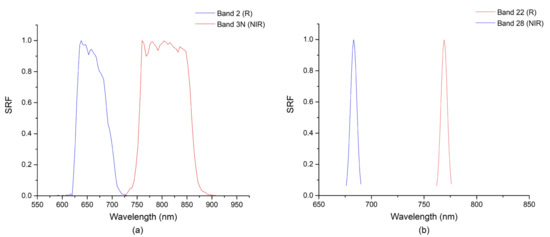
Figure 2.
Spectral response functions of the red and near-infrared bands of ASTER (a) and CASI (b).
In addition to the SRF that has been obtained, the top-of-atmosphere World Radiation Center (WRC) solar spectral curve was selected as the source of ESSI, and can be found on the website (https://staff.aist.go.jp/s.tsuchida/ASTER/cal/info/solar/). The spectral curve is released through ground measurement and rocket flight data. The solar spectral irradiance unit is w•m−2•μm−1. Its spectral range is 350~2500 nm, and its spectral resolution is 1 nm. The BMSI received by each sensor band is calculated by Equation (2), and the ratio is taken, as shown in Table 3. Regarding the ASTER image as the reference, the red band and near-infrared bands of the CASI images were normalized by the ratio of the BMSI between sensors. Then, the spectral normalized CASI red band and the near-infrared band were used to obtain the 1 m NDVI image.
Table 3.
The band mean solar irradiance of the red and near-infrared bands of ASTER and CASI (w•m−2•sr−1•μm−1).
3. Methods
The local variance and the semivariance can be used as methods to analyze the spatial heterogeneity of ground objects. The basic assumptions of the local variance for detecting the spatial pattern size of remote sensing images are that the spatial pattern structure of the remote sensing image is correlated with the size of the features in the scene and the spatial resolution of the remote sensing image. The semivariance method requires the analyzed regionalized variable to satisfy the second-order stationary hypothesis, the intrinsic hypothesis and the normal distribution hypothesis [55,56]. If the data do not meet the normal distribution, they can be converted into a consistent situation. Section 3.1 and Section 3.2 introduce the two methods of the local variance and semivariance, respectively, in detail. Many parameters can be obtained during the analysis process. Among them, the spatial resolution corresponding to the maximum value of the variance in the local variance curve and the range of the semivariance curve are the key analyzed parameters in this article, which is the characteristic scale.
3.1. Local Variance Function
Woodcock et al. [38] first proposed the local variance method to select an appropriate scale or spatial resolution of a dataset by exploring the spatial structure of images. On the one hand, if the spatial resolution of an image is much finer than the objects, most pixel values in the image will be highly correlated with their neighboring pixel values. On the other hand, when the objects approximate the spatial resolution, the neighborhood similarity between the pixel and its surrounding pixels will decrease. With the increase in the spatial resolution, a single resolution unit will contain more objects, and the similarity between most pixel values in the scene and domain pixel values will decrease. This kind of likelihood can be measured by the local variance. The larger the likelihood is, the smaller the local variance. Theoretically, with the increase in spatial resolution, the local variance should first increase, and then decrease gradually. It will reach the peak value at a certain moderate spatial scale. As shown in Figure 3A–C represent different spatial resolutions (A < B < C), and the spatial resolution of point B is directly correlated with the characteristic scale of the ground object. In the actual calculation, a moving window with fixed size (N × N) was set, and each pixel (except those around the edges) in the image can be regarded as the center of the window. The standard deviation in each window was calculated by moving the window continuously on the image, and the mean value of the variance over the whole image was taken as the local variance. The formula is as follows, where the formulas of the mean value f and variance S2 are given in Equations (3) and (4) and where M and N represent the number of rows and columns, respectively, of the image and f(i,j) represents the gray level of the pixel in row i and column j.
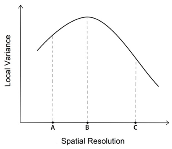
Figure 3.
Theoretical relationship between the spatial resolution and local variance.
To obtain the local variance at each resolution, the images were successively degraded to a coarser spatial resolution by the pixel aggregation resampling method. Furthermore, the local variance under different spatial resolutions of the same image could be computed, and finally, described by the curve. Even though the theoretical graph of the local variance has only one peak, it was found in practical research that ground objects often have multilevel structures, and there may be multiple peak points corresponding to multiple scales.
3.2. Semivariance Function
The semivariance, which is one of the primary tools of geostatistics, characterizes the spatial variation in random variables and measures the autocorrelation of spatial processes. The semivariogram function is related to the distance and direction, indicating the difference in the variable with different positions and directions [57,58,59]. It has been reported that the semivariance can efficiently reflect the structure of spatial continuity due to the potential to describe the spatial variability of images [60]. In this study, as the NDVI of a pixel is highly correlated with the NDVI of its neighboring pixels, this index can be regarded as a continuous and regionalized variable. Thus, semivariograms can be applied to measure the spatial heterogeneity and identify the characteristic scale of the NDVI. Z(x) is assumed to be a localized variable that satisfies the second-order stationarity and characteristic hypothesis. Let the NDVI value of a certain pixel be denoted by Z(x); then, the semivariance γ(h) is defined as one-half of the average squared difference between values separated by h. The specific calculation of γ(h) is given by Equation (5) as follows:
where h is the spatial separation distance between the two sample points; N(h) is the total number of observed data pairs when the lag distance is h; Z(xi) is the measured value of the regionalized variable at point xi; and Z(xi + h) is the value at point xi + h. With the interval distance (h) as the X-axis and the calculated semivariance as the Y-axis, an ideal semivariance theoretical diagram can be constructed as shown in Figure 4.
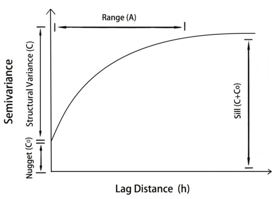
Figure 4.
Theoretical semivariogram.
The semivariance function is based on the “first law of geography”, which states that “everything is related to everything else, but near things are more related than distant things” [61]. Within the range of variation degrees, the variable has a high spatial correlation, and the semivariance increases as h increases. Beyond the degree of variation, the spatial autocorrelation of variables gradually disappears. When the semivariance value reaches a plateau and remains stable, the value is called the sill (C + C0), which is the sum of the total variation in the scene. C is the structural variance. The corresponding h is denoted as the range (A), which is the maximum distance with correlation between sampling points and represents the average distance with spatial autocorrelation of variables. It can be used to identify the characteristic scale of objects. When h equals zero, the semivariance value is called the nugget effect (C0). C0 is the combination of measurement errors and short-scale variations that occur at scales smaller than the distance between the sample values. If there is a large nugget value, A cannot indicate the characteristic scale of the object well [62,63].
In this study, GS+ geostatistical software (version 7.0) was used for NDVI semivariance analysis [64]. To explore the spatial structure of variable variations, it is necessary to fit the actual calculated semivariogram with a mathematical model, such as Linear, Exponential, Gaussian, and Spherical models. GS+ software used by semivariance analysis can automatically select the model with the best-fitting model. Table 4 shows four kinds of semivariogram models. The fitting accuracy depends on the number of point pairs, the sampling distance, and other parameters, and is assessed by the coefficient of determination (R2) of the semivariance models [65]. Two key parameters of the software’s autocorrelation analysis module were set. One parameter is the active lag distance, which refers to the maximum distance, and must be greater than the scale of the object. The default value (approximately 80% of the maximum distance of the sampling point) of the software is unlikely to be the most suitable active lag for the researcher’s data, but we can use this as a reference point to adjust this value to obtain a good-fitting model. The other parameter is the lag class distance interval (separation distance), which defines how the calculated experimental semivariance is grouped into lag classes. Different scales can be obtained by setting different distances according to the type of object. The other analysis parameters adopted default values of the software. It was presumed that the NDVI distribution of the samples in the study area was isotropic, and only the differences caused by different distances were taken into consideration.
Table 4.
Four kinds of semivariogram models.
4. Results and Discussion
4.1. Analysis of the Sample Spatial Heterogeneity in a Small Research Area
On a nonhomogeneous surface, the size of the sample will affect the selection of the data. The smaller the sample range is, the purer the objects that can be obtained. The image extent should be large enough with respect to the spatial features of interest. We used remote sensing images of 1 m resolution and selected samples from a small research area for study. According to the distribution of landscape, three types of typical land features, namely, corn, forest (white poplar, fruit forest, mixed forest areas), and mixed areas (vegetation and buildings), were selected. Three different samples were collected for each type of land. There are nine samples in total, and the size of each sample is 300 m × 300 m (Figure 5).
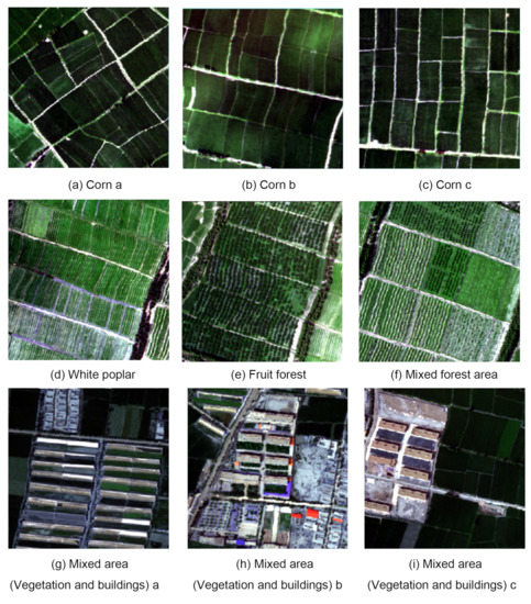
Figure 5.
CASI images of the nine sample areas of the three typical features (R: Band 8; G: Band 13; B: Band 20). Subfigure (a–c) are three different types of corn field samples. (d–f) represent the sample of white poplar, fruit forest and mixed forest area respectively. (g–i) show three different types of mixed area.
For the local variance analysis, taking 2 m as the resampling interval, 1 m CASI NDVI images of the nine samples were resampled to degrade the spatial resolution to 19 m and images of 1 m, 3 m, 5 m, 7 m, 9 m, 11 m, 13 m, 15 m, 17 m, and 19 m spatial resolutions were acquired. The local variance under the sliding window of each scene image (3 × 3) was calculated, and graphs of the local variance of the three typical features were obtained and are shown in Figure 6. The local variance results were analyzed separately according to three kinds of objects:
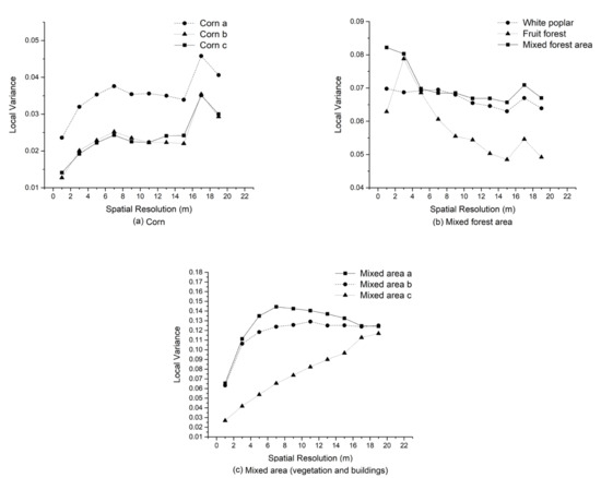
Figure 6.
Local variance curves of the three kinds of typical objects. Subfigure (a–c) represent corn, forest and mixed area respectively.
- (1)
- As shown in Figure 6a, the local variances of the three samples of corn are lower (approximately 0.01–0.05) than those of the other objects. Although the local variance of corn sample a is obviously higher than that of the other two samples, the varying trends in the three local variances are consistent, which means that the overall spatial heterogeneity of this sample is much stronger, indicating that this corn field grows slightly unevenly. The local variances of the three samples are all low at the initial resolution and then increase gradually with increasing spatial resolution. This trend continues until a small peak is found at a spatial resolution of 7 m. When the spatial resolution changes from 7 m to 15 m, the local variances trend slightly downward. After this flat region, the local variances increase rapidly, and a new peak appears at a spatial resolution of 17 m. This peak is more noticeable than the first peak at 7 m. Different from the theoretical hypothesis, the local variance curve of pure corn has two peaks corresponding to two characteristic scales: 7 m and 17 m. A peak appeared in the local variance of 17 m, indicating that with the increase in the pixel size of the image, the target ground object of the study changed. The sample contains only corn class, and the fields are arranged in clumps. It maybe indicates that the feature type has changed from a small corn field to a large corn field.
- (2)
- The local variances of the forest areas are approximately 0.04–0.08. Figure 5e,f show that the spatial distribution of the white poplar, fruit forest, and mixed areas (vegetation and buildings) presents a regular row structure. However, the trends in the local variance of the three samples are distinctly different. As you can see in Figure 6b, the local variances of the white poplars decrease with the increasing resolution, and the curve changes slightly. It was originally assumed that the peak would appear when the resolution is close to the size of the objects. However, there was no obvious peak for white poplars. One possible reason is that the crown diameter of a single poplar tree is considerably smaller than the original fine resolution cells, and thus, the type of ground object studied shifted to the poplar forest rather than a single tree. Another probable cause is that this area is relatively flat, and the growth state of the forest is so homogeneous that there is not one size dominant enough to cause a peak. Thus, we can regard that the scale of the white poplars is approximately 1–7 m. The local variance of the fruit forest is lower at 1 m, but suddenly increases when the spatial resolution degrades to 3 m, resulting in a peak. As the resolution increases past the peak, the variance decreases sharply and shows no upward trend. Naturally, the scale of the fruit forest is approximately 3 m. Unlike white poplar trees, the canopy diameter of a single fruit tree is large, so the tree can be detected by a local variance graph. The mixed forest area encompasses several different sizes of vegetation. The curve starts with a high local variance at 1–3 m, and the local variance goes down rapidly between a resolution of 3 m and 5 m. Finally, the curve shows a gentle downward trend. The peak of this mixed area is considered to be 1–3 m, that is, the scale of the feature.
- (3)
- For the vegetation and building mixed area, the local variance of the three types of samples is approximately 0.02–0.16 in Figure 6c. The local variance curves of mixed areas A and B are more similar than those of a/c and b/c. With the increase in resolution, the local variances for these areas first increase and then decline. Therefore, the scales of the two samples are 7 m and 11 m, respectively. However, the local variances of mixed area C continuously increase as the resolution increases. The lack of a definite peak implies that there is not a distinct object that dominates the scene due to the limitation of the research range. The scale of the sample is not within the range of 1 m to 19 m. As mentioned earlier, image degradation will lead to a reduction in the number of pixels in the image, while local variance analysis requires a lower limit of the number. Therefore, the scope of research will be restricted to a certain extent. If the range of the study area can subsequently be extended and the pixel of the downsampled image is coarser, a peak value may be obtained.
Additionally, semivariance analysis of the samples was performed to compare with the local variance results. Four different separation distances (h) of 1 m, 5 m, 10 m, and 15 m were set to study the experimental semivariograms of the nine samples. GS+ software used by semivariance analysis can automatically select the best-fitting model. Table 5, Table 6, Table 7 and Table 8 show the parameters of the optimal fitting model for the semivariance analysis of different samples. This can be seen that the Exponential model is the best choice for all sample fitting in the semivariance analysis in this study. The models were built in the software, and the three crucial parameters of the function were obtained: A0, C0 + C, and C0. A0 needs to be converted to A, and different models have different conversion formulas [64]. It was found that the semivariogram results of the three corn samples are highly similar, so only the fitting result of corn sample a was selected for presentation. Its lag distance is 180 m, and Table 5 describes the fitting model parameters of corn sample a. For the forestlands, the analysis results of the semivariogram of each sample are different, which depend on the characteristics and distribution of vegetation. The lag distances of white poplar, fruit forests, and forest mixed areas are 192 m, 180 m, and 180 m, respectively (Table 6). In light of the results from Table 7, for the mixed area (vegetation and buildings), the fitting results of the different samples vary greatly, which requires the specific analysis of the individual samples. The lag distances of the three mixed area samples are all approximately 190 m. In addition, the curve of A in the process of h changing from a resolution of 1 m to a resolution of 15 m for the different types of ground objects is shown in Figure 7 to facilitate a more intuitive analysis.
Table 5.
Parameters of the semivariogram optimal fitting models of corn sample A.
Table 6.
Parameters of the semivariogram optimal fitting models of the three types of forest samples.
Table 7.
Parameters of the semivariogram optimal fitting models of mixed areas (vegetation and buildings).
Table 8.
Parameters of the semivariogram optimal fitting models of 600 m × 600 m areas of the typical samples.
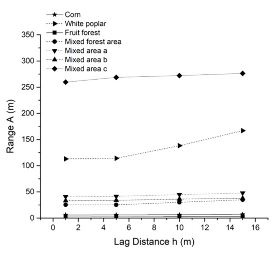
Figure 7.
Variation diagram of Ranges (A) of different ground objects at different lag distance (h).
It can be seen from Table 5, Table 6 and Table 7 and Figure 7 that the Exponential model provided the best fit for all the semivariogram models of the samples. The A values of the different ground objects have different variation trends under different h values. The A of corn is approximately 6–7 m. The A of the fruit forest is approximately 3 m, and the curve of variation is closest to the level among all types of ground objects in the study area. The variation range of the A values for the white poplars was the largest at different h values, with A increasing from 115 m to 170 m. The characteristic scales corresponding to mixed areas a, b, and c are 40–50 m, 30–40 m, and 250–280 m, respectively. The results show that the scale of corn and fruit forest was small, that of mixed forest was medium, and that of white poplar was large. The scales of the mixed samples have both high and low values. The C0 values of all samples are less than 0.03, indicating that the NDVI variability arising from measurement errors was small. The C0 + C values of corn and the fruit forest are the lowest, indicating that the total spatial variation degree in the NDVI is the lowest. The C0 + C of the mixed area (vegetation and buildings) is the highest, and the total spatial variation degree is the highest.
4.2. Analysis of the Heterogeneity on the Scale of Expanded Research
The previous study conducted a spatial heterogeneity analysis and characteristic scale extraction within the range of 300 m × 300 m derived from 1-m CASI NDVI data. The scope of this research was extended to the range of 600 m × 600 m. In addition, 15 m ASTER NDVI data were introduced for comparison to study the spatial distribution patterns of corn, forest and mixed (vegetation and building) areas. Data samples need to be collected again. In Section 3.1, it was found that there was a high similarity between corn samples, while the samples in the mixed region were significantly different from each other. There are no pure poplar or fruit trees in this large area, and only the mixed forest can be found. A total of five samples, including a pure corn field, a forest, and three vegetation and building mixed areas, were selected in pre-experiment. Because different samples of the mixed area contain different types of ground objects, the differences between samples are large. Only one mixed sample was selected as the case of analysis and demonstration. Therefore, only three samples were selected and shown in the study (corn, forest, and mixed areas (vegetation and buildings)). The CASI images of these samples are shown in Figure 8.
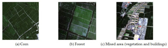
Figure 8.
CASI images of the three typical features (R: Band 8; G: Band 13; B: Band 20). Subfigure (a–c) represent corn, forest and mixed area respectively.
Similarly, ASTER NDVI data were sampled down to 29 m at 2 min intervals. CASI NDVI images with 1 m, 5 m, 9 m, 13 m, 17 m, 19 m, 21 m, 23 m, 25 m, 27 m, and 29 m resolutions and ASTER NDVI images with 15 m, 17 m, 19 m, 21 m, 23 m, 25 m, 27 m, and 29 m resolutions could be acquired. After resampling the two images in this way, the resolution of the two types of data can be guaranteed to remain the same after 17m. The local variances of each image were calculated by using a 3 × 3 sliding window, and the local variance curves are shown in Figure 9.
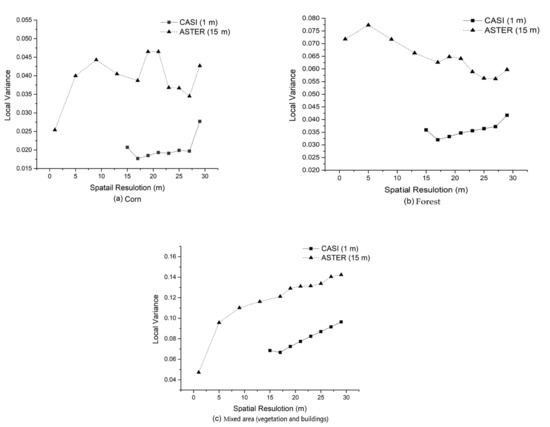
Figure 9.
Local variance curves of the CASI (1 m) and ASTER (15 m) NDVI images of the three samples. Subfigure (a–c) represent corn, forest and mixed area respectively.
According to the corn sample in Figure 9a, the variation trend in the local variance derived from the original 1 m CASI image is different from that derived from the original 15 m ASTER image. Within the range of 1 m to 29 m, there are multiple peaks corresponding to multiple scales in the local variance curve of the original 1 m image. Due to the limitations of the initial resolution, the entire curve cannot be shown. It is not known whether 29 m is also a peak point, so it can be inferred only that the scale of corn in this image is between 9 m and 20 m. The peak cannot be observed from the local variance curve of the 15 m initial image, so the scale of corn could not be detected. For forestland (Figure 9b), the local variance of the 1 m initial image first increases and then decreases with the addition of spatial resolution. The peak value is approximately 5 m. The local variance curve of the initial 15 m image decreases first, and then increases with increasing spatial resolution. The local variances for spatial resolutions less than 15 m and greater than 29 m cannot be acquired in the figure. Thus, the peak value and scale of this sample could not be detected. As shown in Figure 9c, for the mixed area (vegetation and buildings), the local variances of the original 1 m and 15 m images increase gradually as the spatial resolution increases. Neither of these images can be used to identify the scale of the mixed area.
These graphs have demonstrated that the use of moderate-resolution (15 m) raw images for the local variance is not effective. For fine objects, such as single white poplar and fruit trees, the size of a 15 m resolution pixel is far larger than the size of trees. It can be seen in the corn and forest samples that the trend in the two curves in the same image varies greatly within the same resolution range.
The semivariance analyses of 15 m ASTER NDVI images were carried out in GS+, and the lag and separation distances were selected according to the pre-experiment. Then, the variation functions of the NDVI data in the three sample regions were calculated, and the best-fitting model was selected, as shown in Table 8. The A’s of corn, forest, and the mixed area (vegetation and buildings) are 23.1, 43.6, and 56.8 m, which is the scale corresponding to the three types of samples.
5. Conclusions
In this paper, the core observation area in the middle reaches of the HRB was taken as the study area. Local variance and semivariance analysis methods are proposed for comparative analysis to explore the spatial heterogeneity and identify the characteristic scale of typical features in the artificial irrigation oasis. The results of the two methods were obtained for remote sensing images of five ground objects of two spatial resolutions. Furthermore, the results of the characteristic scale analysis of several ground objects of the two methods and different scopes are summarized in Table 9. The following conclusions can be drawn:
Table 9.
Summary of the characteristic scale of each ground object under the different methods and different research scopes.
- (1).
- In nature, ground objects have multi-hierarchical structures. The research scale determines the type of ground objects to be detected. In this research, the spatial heterogeneity of corn is the lowest, followed by that of the forest and mixed areas (vegetation and buildings). The corn field has scales of 7 m and 20 m. A single white poplar is taken as the studied object with a scale of 1–7 m. If the studied object has shifted into blocks, its scale becomes 120–170 m. For the fruit trees, the crown diameters are relatively large. As seen from the 1 m high-resolution remote sensing image, the distance between single fruit trees also spans several pixels in the image. In our study, the studied object always corresponds to a single fruit tree, and the only scale is 3 m. For the mixed forest area, the scale of the local variance analysis is 1–5 m and that of the semivariance analysis is 25–40 m. For the mixed area (vegetation and buildings), the degree of spatial heterogeneity is the largest. Different samples have different characteristic scales, which need to be analyzed according to the specific features contained. It is also found that with the expansion of the research scope, the scales of all studied objects have increased to varying degrees. As the pixel resolution gets coarser, if the scale of some fine objects is smaller than the pixel resolution, their spatial structure cannot be detected, but the spatial distribution information of larger target features can be obtained. This is also one of the evidences of the existence of multi-scale structure of surface features, that is, the results of the research problems will change with the changes of scales.
- (2).
- Local variance analysis derived from the 15 m ASTER NDVI image barely detected the scale. This phenomenon might be caused by the fact that the scale of the ground object was not within the resolution range of the experimental image. Local variance analysis is not suitable for low or medium spatial-resolution remote sensing images as the basis image. If the scale of the research object itself is less than 15 m, the local variance method based on the original image with medium or low resolution cannot detect the scale of the object. For the semivariance analysis, regardless of the scale of the remote sensing data, a corresponding variation value will be given. Therefore, the 15 m ASTER NDVI image can be used in a semivariance analysis. However, does the range value necessarily represent the size of the sample? It is obvious that this range is meaningless for complex samples that contain more than one feature. There is no unified characteristic scale for mixed ground objects. Researchers need to determine the characteristic value according to the specific type and distribution of surface features contained in the sample. Relevant research has found that the global variation in complex images is often greater than that of individual ground object classes in the images [66].
- (3).
- Both local variance analysis and semivariance analysis can be used for spatial heterogeneity analysis and characteristic scale extraction. For a single object of identifiable size, the scale results obtained by the two methods are relatively consistent. The scale obtained by the local variance analysis is relatively small. It indicates that the target size identified by local variance is smaller. For example, the local variance of mixed forestland is 1–5 m, while the semivariance is 25–40 m. Nevertheless, for an object of indistinguishable size or continuous distribution, the scales obtained by the two methods are different. Local variance and semivariance are similar in mechanism and are maneuverable to facilitate researchers to quickly select the appropriate spatial resolution of remote sensing data according to the research area. However, compared with the local variance method, the semivariance method does not need to gradually reduce the resolution of the image; instead, the different values of the lag distance or separation distance of only one image need to be set. It can reduce the complexity of the experiment. In this study, the local variance analysis took 2 m as the sampling interval, so the obtained scale had an error of ±1 m. When a peak does not appear in the local variance curve, it is difficult to identify the corresponding scale. Due to the limited sample size and the limited resolution of the lower resolutions, the detection range is restricted. The semivariance analysis can obtain a corresponding range value of any image. Except for complicated samples, the obtained scale is not applicable. For pure fine features, this method is more efficient. In summary, the semivariance method has more advantages than the local variance method in the description of the overall spatial heterogeneity, the acquisition of multiscale levels, and the convenience of calculation.
The significance of this paper for the study of the appropriate spatial resolution of remote sensing images lies in the use and discussion of methods and experimental consideration, rather than the comparison of whether the results of local variance and semivariance are completely equal for the scale of the same object. If the research area or experimental samples are replaced, the actual scale calculation results obtained for the same object may also be different. The scale analysis of ground features, that is, the selection of the spatial resolution of the images, will directly affect the results of the analysis and the application. This article indicates that with a small research area of uniform objects, the local variance and semivariance are maneuverable to facilitate researchers to quickly select the appropriate spatial resolution of remote sensing data according to the research area. Nevertheless, there are many types of ground objects in images of complex samples, so it is far from sufficient to determine the optimal scale of only one type of ground object. It is difficult to satisfy the needs of multi-type information extraction. It will be more important to consider the classification of complex sample features, analyze the change process of different features, and comprehensively analyze the size of complex samples. Most of the previous studies can only detect the single scale of surface features and can only compare the characteristic values of different features. While this study not only to detect the characteristic scale of different object also detected the same object types of multi-scale structure. Although it cannot obtain the full scale of the feature scale, it can also help to understand the property of continuous change of feature in spatial pattern. It provides the train of thought for multi-scale detection research.
Studying the scale of ground objects is conducive to determining the level of spatial resolution to which the data scale is converted to correctly reveal the law of spatial distribution or change in features. However, the identification of scales of features has only been compared by different methods, and there is no benchmark for verification. We think that the verification of scale requires the actual or indirect measurement data of ground objects to carry out reasonable verification. Ground objects with obvious shapes or regular distributions, such as fruit forests arranged in obvious row spacing. Whether the row spacing of the image can be measured based on the high-resolution images, and the row spacing of the features can be calculated and it can be used as reference data for the characteristic scale of the fruit forest. However, this method is not suitable for continuous distribution objects, which are not easy to measure. Perhaps we can combine the scale conversion to convert the initial resolution image to the appropriate spatial resolution to see if the distribution law of the geographical objects can be obtained, so as to check whether the size of the characteristic scale derived is reasonable. It needs to be validated in conjunction with the scale transformation. This issue should be further studied and discussed in the future.
Author Contributions
W.Y. outlined the research topic and assisted in writing the manuscript. M.M. provided helpful suggestions on the research design. X.L. and W.W. provided helpful suggestions for revising the work. J.S. collected and preprocessed all the data. X.W. processed the data, analyzed the results and wrote the manuscript. All authors have read and agreed to the published version of the manuscript.
Funding
This study was supported by the National Major Projects on High-Resolution Earth Observation System (grant number: 21-Y20B01-9001-19/22), the China Postdoctoral Science Foundation (grant number: 2020M670542) and the Fundamental Research Funds for the Central Universities of China (grant number: XDJK2014C012), and the Natural Science Foundation of China (grant number: 41830648).
Institutional Review Board Statement
Not applicable.
Informed Consent Statement
Not applicable.
Data Availability Statement
The main remote sensing data were downloaded from the National Tibetan Plateau Data Center (http://data.tpdc.ac.cn/en/).
Acknowledgments
The authors would thank all the institutes and universities involved in the observation experiment for their sharing the data. We also would like to thank the staffs of National Tibetan Plateau Data Center for providing the data and their patient answers to the questions raised during the data application process.
Conflicts of Interest
The authors declare no conflict of interest.
References
- Wu, J.; Vankat, J. A system dynamics model of island biogeography. Bull. Math. Biol. 1991, 53, 911–940. [Google Scholar] [CrossRef]
- Wu, J.; Loucks, O.L. From Balance of Nature to Hierarchical Patch Dynamics: A Paradigm Shift in Ecology. Q. Rev. Biol. 1995, 70, 439–466. [Google Scholar] [CrossRef]
- Legendre, P.; Fortin, M.J. Spatial pattern and ecological analysis. Vegetatio 1989, 80, 107–138. [Google Scholar] [CrossRef]
- Li, J.; Song, C.; Cao, L.; Zhu, F.; Meng, X.; Wu, J. Impacts of landscape structure on surface urban heat islands: A case study of Shanghai, China. Remote Sens. Environ. 2011, 115, 3249–3263. [Google Scholar] [CrossRef]
- Herold, M.; Woodcock, C.; Loveland, T.; Townshend, J.; Brady, M.; Steenmans, C.; Schmullius, C. Land-Cover Observations as Part of a Global Earth Observation System of Systems (GEOSS): Progress, Activities, and Prospects. IEEE Syst. J. 2008, 2, 414–423. [Google Scholar] [CrossRef]
- Pickett, S.T.A.; Cadenasso, M.L. Landscape Ecology: Spatial Heterogeneity in Ecological Systems. Science 1995, 269, 331–334. [Google Scholar] [CrossRef]
- Sadowski, F.G.; Malila, W.A.; Sarno, J.E.; Nalepka, R.F.J.R. The Influence of Multispectral Scanner Spatial Resolution on Forest Feature Classification. In Proceedings of the Eleventh International Symposium on Remote Sensing of Environment, Houston, TX, USA, 1 January 1977; Volume 2. [Google Scholar]
- Freek, V.D.M.; Bakker, W.; Scholte, K.; Skidmore, A.; De Jong, S.; Dorresteijn, M.; Clevers, J.; Epema, G.J.G.I. Scaling to the MERIS Resolution: Mapping Accuracy and Spatial Variability. Geocarto Int. 2000, 15, 39–50. [Google Scholar]
- Wu, J.; Shen, W.; Sun, W.; Tueller, P.T. Empirical patterns of the effects of changing scale on landscape metrics. Landsc. Ecol. 2002, 17, 761–782. [Google Scholar] [CrossRef]
- Drăgut, L.; Tiede, D.; Levick, S.R. ESP: A tool to estimate scale parameter for multiresolution image segmentation of remotely sensed data. Int. J. Geogr. Inf. Sci. 2010, 24, 859–871. [Google Scholar] [CrossRef]
- Lam, N.S.N.; Quattrochi, D.A. On the Issues of Scale, Resolution, and Fractal Analysis in the Mapping Sciences. Prof. Geogr. 1992, 44, 88–98. [Google Scholar] [CrossRef]
- Schneider, D.C. The Rise of the Concept of Scale in Ecology. BioScience 2001, 51, 545. [Google Scholar] [CrossRef]
- O’Neil, R.J.E.S. Homage to St. Michael: Or, Why Are There So Many Books on Scale? Columbia University Press: New York, NY, USA, 1998. [Google Scholar]
- McCarthy, A.J. The Irish National Electrification Scheme. Geographical Review. Geogr. Rev. 1957, 47, 539–554. [Google Scholar] [CrossRef]
- Weiss, M.; Baret, F.; Myneni, R.B.; Pragnère, A.; Knyazikhin, Y. Investigation of a model inversion technique to estimate canopy biophysical variables from spectral and directional reflectance data. Agronomie 2000, 20, 3–22. [Google Scholar] [CrossRef]
- Marceau, D.J. The Scale Issue in the Social and Natural Sciences. Can. J. Remote Sens. 1999, 25, 347–356. [Google Scholar] [CrossRef]
- Silvestri, S.; Marani, M.; Settle, J.; Benvenuto, F.; Marani, A. Salt marsh vegetation radiometry: Data analysis and scaling. Remote Sens. Environ. 2002, 80, 473–482. [Google Scholar] [CrossRef]
- Wu, J.; Jelinski, D.E.; Luck, M.; Tueller, P.T. Multiscale Analysis of Landscape Het-erogeneity: Scale Variance and Pattern Metrics. Geogr. Inf. Sci. 2000, 6, 6–19. [Google Scholar]
- Wiens, J.A. Spatial Scaling in Ecology. Funct. Ecol. 1989, 3, 385. [Google Scholar] [CrossRef]
- Li, H.; Reynolds, J.F. A Simulation Experiment to Quantify Spatial Heterogeneity in Categorical Maps. Ecology 1994, 75, 2446. [Google Scholar] [CrossRef]
- Bian, L.; Walsh, S.J. Scale Dependencies of Vegetation and Topography in a Moun-tainous Environment of Montana. Prof. Geogr. 1993, 45, 1–11. [Google Scholar] [CrossRef]
- Kotliar, N.B.; Wiens, J.A. Multiple Scales of Patchiness and Patch Structure: A Hierarchical Framework for the Study of Heterogeneity. Oikos 1990, 59, 253. [Google Scholar] [CrossRef]
- Wu, J. Hierarchy and Scaling: Extrapolating Information along a Scaling Ladder. Can. J. Remote Sens. 1999, 25, 367–380. [Google Scholar] [CrossRef]
- Seydi, S.T.; Hasanlou, M.; Amani, M. A New End-to-End Multi-Dimensional CNN Framework for Land Cover/Land Use Change Detection in Multi-Source Remote Sensing Datasets. Remote Sens. 2020, 12, 2010. [Google Scholar] [CrossRef]
- Goddijn-Murphy, L.; Williamson, B.J. On Thermal Infrared Remote Sensing of Plastic Pollution in Natural Waters. Remote Sens. 2019, 11, 2159. [Google Scholar] [CrossRef]
- Yang, X.; Xu, B.; Jin, Y.; Qin, Z.; Ma, H.; Li, J.; Zhao, F.; Chen, S.; Zhu, X. Remote sensing monitoring of grassland vegetation growth in the Beijing–Tianjin sandstorm source project area from 2000 to 2010. Ecol. Indic. 2015, 51, 244–251. [Google Scholar] [CrossRef]
- Justice, C.O.; Holben, B.N.; Gwynne, M.D. Monitoring East African vegetation using AVHRR data. Int. J. Remote Sens. 1986, 7, 1453–1474. [Google Scholar] [CrossRef]
- Costantini, M.L.; Zaccarelli, N.; Mandrone, S.; Rossi, D.; Calizza, E.; Rossi, L. NDVI spatial pattern and the potential fragility of mixed forested areas in vol-canic lake watershed. For. Ecol. Manag. 2012, 285, 133–141. [Google Scholar] [CrossRef]
- Balaguer-Beser, A.; Ruiz, L.A.; Hermosilla, T.; Recio, J.A. Using semivario-gram indices to analyse heterogeneity in spatial patterns in remotely sensed images. Comput. Geosci. 2013, 50, 115–127. [Google Scholar] [CrossRef]
- Zaccarelli, N.; Riitters, K.H.; Petrosillo, I.; Zurlini, G. Indicating disturbance content and context for preserved areas. Ecol. Indic. 2008, 8, 841–853. [Google Scholar] [CrossRef]
- Kolasa, J.; Pickett, S.T.A. Ecological Heterogeneity; Springer: New York, NY, USA, 1992; p. 86. [Google Scholar]
- Gustafson, E.J. Quantifying Landscape Spatial Pattern: What Is the State of the Art? Ecosystems 1998, 1, 143–156. [Google Scholar] [CrossRef]
- Read, J.M.; Lam, N.S.N. Spatial methods for characterising land cover and detecting land-cover changes for the tropics. Int. J. Remote Sens. 2002, 23, 2457–2474. [Google Scholar] [CrossRef]
- Sugihara, G.; May, R.M. Applications of fractals in ecology. Trends Ecol. Evol. 1990, 5, 79–86. [Google Scholar] [CrossRef]
- Atkinson, P.M.; Curran, P.J. Choosing an appropriate spatial resolution for remote sensing investigations. Photogramm. Eng. Remote Sens. 1997, 63, 1345–1351. [Google Scholar]
- Ming, D.P.; Wang, Q.; Yang, J.Y. Spatial Scale of Remote Sensing Image and Selection of Optimal Spatial Resolution. J. Remote Sens. 2008, 12, 529–537. [Google Scholar]
- Han, P.; Gong, J.Y.; Li, Z.L.; Bo, Y.C.; Cheng, L. Selection of optimal scale in re-motely sensed image classification. J. Remote Sens. 2010, 14, 507–518. [Google Scholar]
- Woodcock, C.E.; Strahler, A.H. The factor of scale in remote sensing. Remote Sens. Environ. 1987, 21, 311–332. [Google Scholar] [CrossRef]
- Webster, R. Quantitative Spatial Analysis of Soil in the Field; Springer: New York, NY, USA, 1985; pp. 1–70. [Google Scholar]
- Li, H.; Reynolds, J.F. On definition and quantification of heterogeneity. Oikos 1995, 73, 280–284. [Google Scholar] [CrossRef]
- Atkinson, P.M.; Tate, N.J. Spatial Scale Problems and Geostatistical Solutions: A Review. Prof. Geogr. 2000, 52, 607–623. [Google Scholar] [CrossRef]
- Sanderson, E.W.; Zhang, M.; Ustin, S.L.; Rejmankova, E. Geostatistical scaling of canopy water content in a California salt marsh. Landsc. Ecol. 1998, 13, 79–92. [Google Scholar] [CrossRef]
- Meisel, J.E.; Turner, M.G. Scale detection in real and artificial landscapes using semi-variance analysis. Landsc. Ecol. 1998, 13, 347–362. [Google Scholar] [CrossRef]
- Atkinson, P.M.; Curran, P. Defining an optimal size of support for remote sensing investigations. IEEE Trans. Geosci. Remote Sens. 1995, 33, 768–776. [Google Scholar] [CrossRef]
- Lathrop, R.G.; Pierce, L.L. Ground-based canopy transmittance and satellite remotely sensed measurements for estimation of coniferous forest canopy structure. Remote Sens. Environ. 1991, 36, 179–188. [Google Scholar] [CrossRef]
- Li, X.; Cheng, G.; Liu, S.; Xiao, Q.; Ma, M.; Jin, R.; Che, T.; Liu, Q.; Wang, W.; Qi, Y.; et al. Heihe Watershed Allied Telemetry Experimental Research (HiWATER): Scientific Objectives and Experimental Design. Bull. Am. Meteorol. Soc. 2013, 94, 1145–1160. [Google Scholar] [CrossRef]
- Hua, Z.; Bo, Z. Study of environment restoration after Water-distribution project in lower reaches of Heihe River. In Proceedings of the 2011 International Symposium on Water Resource and Environmental Protection, Xi’an, China, 20–22 May 2011. [Google Scholar]
- Li, X.; Liu, S.; Xiao, Q.; Ma, M.; Jin, R.; Che, T.; Wang, W.; Hu, X.; Xu, Z.; Wen, J.J.D. A multiscale dataset for understanding complex eco-hydrological processes in a heterogeneous oasis system. Sci. Data 2017, 4, 170083. [Google Scholar] [CrossRef] [PubMed]
- Zhang, M. HiWATER: Land Cover Map in the Core Experimental Area of Flux Observation Matrix; National Tibetan Plateau Data Center: Beijing, China, 2017. [Google Scholar] [CrossRef]
- Zhihui, W.; Liangyun, L. Monitoring on Land Cover Pattern and Crops Structure of Oasis Irrigation Area of Middle Reaches in Heihe River Basin Using Remote Sensing Data. Earth Sci. 2013, 28, 948–956. [Google Scholar]
- Hu, S.S.; Zhang, L.F.; Zhang, X.; Wang, Q.; Han, B.; Zhang, N. Calculation and Reliability Analysis of Satellite Sensors Band Solar Irradiance. Remote Sens. Land Resour. 2012, 94, 97–102. [Google Scholar]
- Smith, M.S. How to Convert ASTER Radiance Values to Reflectance. An Online Guide; University Idaho: Moscow, ID, USA, 2007. [Google Scholar]
- Ricchiazzi, P.; Yang, S.; Gautier, C.; Sowle, D. SBDART: A Research and Teaching Software Tool for Plane-Parallel Radiative Transfer in the Earth’s Atmosphere. Bull. Am. Meteorol. Soc. 1998, 79, 2101–2114. [Google Scholar] [CrossRef]
- Teillet, P.M.; Barker, J.L.; Markham, B.L.; Irish, R.R.; Fedosejevs, G.; Storey, J.C. Radiometric cross-calibration of the Landsat-7 ETM+ and Landsat-5 TM sensors based on tandem data sets. Remote Sens. Environ. 2001, 78, 39–54. [Google Scholar] [CrossRef]
- Cormack, R.M.; Cressie, N.J.T.N. Statistics for Spatial Data; John Wiley & Sons, Inc.: Hoboken, NJ, USA, 2010; Volume 4, pp. 613–617. [Google Scholar] [CrossRef]
- Isaaks, E.H.; Srivastava, M.R. An Introduction to Applied Geostatistics; Oxford University Press: New York, NY, USA, 1989. [Google Scholar]
- Matheron, G. Principles of geostatistics. Econ. Geol. 1963, 58, 1246–1266. [Google Scholar] [CrossRef]
- Curran, P.J.; Atkinson, P.M. Geostatistics and remote sensing. Prog. Phys. Geogr. 1998, 22, 61–78. [Google Scholar] [CrossRef]
- Duveiller, G.; Defourny, P. A conceptual framework to define the spatial resolution requirements for agricultural monitoring using remote sensing. Remote Sens. Environ. 2010, 114, 2637–2650. [Google Scholar] [CrossRef]
- Guedes, I.C.D.L.; Mello, J.M.D.; Silveira, E.M.D.O.; Mello, C.R.D.; Reis, A.A.D.; Gomide, L.R. Continuidade espacial de características dendrométricas em povoamentos clonais de Eucalyptus sp. avaliada ao longo do tempo. Cerne 2015, 21, 527–534. [Google Scholar] [CrossRef]
- Tobler, W.R. A Computer Movie Simulating Urban Growth in the Detroit Region. Econ. Geogr. 1970, 46, 234. [Google Scholar] [CrossRef]
- Treitz, P.; Howarth, P. High Spatial Resolution Remote Sensing Data for Forest Ecosystem Classification: An Examination of Spatial Scale. Remote Sens. Environ. 2000, 72, 268–289. [Google Scholar] [CrossRef]
- Hu, X.; Hong, W.; Qiu, R.; Hong, T.; Chengzhen, W.; Wu, C. Geographic variations of ecosystem service intensity in Fuzhou City, China. Sci. Total Environ. 2015, 215–226. [Google Scholar] [CrossRef]
- Robertson, G.P. Geostatistics for the Environmental Sciences: GS+ User’s Guide; Gamma Design Software: Plainwell, MI, USA, 1998; pp. 68–94. ISBN 0-9707410-0-6. [Google Scholar]
- Davis, J.C.J.B. Statistics and Data Analysis in Geology. Biometrics 1988, 44, 526–527. [Google Scholar] [CrossRef]
- Zhu, J.X.; Wang, J.L. Appropriate Scale Extraction from Complicated Scene Model Based on Semivariogram Analysis. Geogr. Geo-Inf. Sci. 2015, 31, 33–37. [Google Scholar]


Publisher’s Note: MDPI stays neutral with regard to jurisdictional claims in published maps and institutional affiliations. |
© 2021 by the authors. Licensee MDPI, Basel, Switzerland. This article is an open access article distributed under the terms and conditions of the Creative Commons Attribution (CC BY) license (http://creativecommons.org/licenses/by/4.0/).