Abstract
Haze and dust pollution have a significant impact on human production, life, and health. In order to understand the pollution process, the study of these two pollution characteristics is important. In this study, a one-year observation was carried out at the Beijing Southern Suburb Observatory using the MAX-DOAS instrument, and the pollution characteristics of the typical haze and dust events were analyzed. First, the distribution of aerosol extinction (AE) and H2O concentrations in the two typical pollution events were studied. The results showed that the correlation coefficient (r) between H2O and AE at different heights decreased during dust processes and the correlation slope (|k|) increased, whereas r increased and |k| decreased during haze periods. The correlation slope increased during the dust episode due to low moisture content and increased O4 absorption caused by abundant suspended dry crustal particles, but decreased during the haze episode due to a significant increase of H2O absorption. Secondly, the gas vertical column density (VCD) indicated that aerosol optical depth (AOD) increased during dust pollution events in the afternoon, while the H2O VCD decreased; in haze pollution processes, both H2O VCD and AOD increased. There were significant differences in meteorological conditions during haze (wind speed (WD) was <2 m/s, and relative humidity (RH) was >60%) and dust pollution (WD was >4 m/s, and RH was <60%). Next, the vertical distribution characteristics of gases during the pollution periods were studied. The AE profile showed that haze pollution lasted for a long time and changed slowly, whereas the opposite was true for dust pollution. The pollutants (aerosols, NO2, SO2, and HCHO) and H2O were concentrated below 1 km during both these typical pollution processes, and haze pollution was associated with a strong temperature inversion around 1.0 km. Lastly, the water vapor transport fluxes showed that the water vapor transport from the eastern air mass had an auxiliary effect on haze pollution at the observation location. Our results are of significance for exploring the pollution process of tropospheric trace gases and the transport of water vapor in Beijing, and provide a basis for satellite and model verification.
1. Introduction
Air pollution has become a serious environmental problem in China, especially in economically developed and densely populated areas, such as Beijing–Tianjin–Hebei [1,2,3]. Beijing is a megacity, with a large population and numerous vehicles; it has frequently suffered from haze pollution in recent years, especially during winter [4,5,6]. In addition, the transport of dust from the northwest aggravates the pollution in Beijing during the spring. The inhalation of aerosols from haze and dust during heavy pollution outbreaks has noticeably adverse effects on human health. Studies have shown that millions of people die prematurely every year due to outdoor air pollution [7]. Moreover, air pollution plays a role in COVID-19 transmission [8,9,10]. Therefore, there has been an enhanced focus on haze and dust pollution in China.
Meteorological conditions are cofactors in the formation of haze and the transportation of atmospheric pollutants [11,12,13]. Water vapor is a natural greenhouse gas, which not only affects the frequency of precipitation, but also participates in a variety of atmospheric chemical reactions [14,15]. The local meteorological conditions during the winter haze in the Beijing–Tianjin–Hebei region are usually accompanied by high relative humidity (RH) [16]. Water vapor is a cofactor that causes haze, and an increase in water vapor concentrations effectively promotes the formation of secondary aerosols. In conditions of low wind speed, pollutants cannot effectively diffuse, further aggravating the pollution [17,18,19]. Strong winds allow the transport of dust from distant sources, while low RH means minimal precipitation to wash the dust out of the atmosphere, thus providing favorable environmental conditions for the dust events [20,21]. Therefore, whether investigating haze pollution or dust pollution, it is of great significance to study the variations in local water vapor concentration in the pollution process.
Although several studies have been conducted on the characteristics of haze pollution [5,6,16,19] and dust pollution [20,21,22] via near-ground observations or large-scale models, the vertical distribution studies of the two types of pollution characteristics remain rare. Zhou et al. (2012) studied the concentration and chemical composition of fine particles during haze and dust pollution in Shanghai in autumn, and found that the secondary components of haze pollution have a greater contribution to PM2.5, whereas dust pollution is dominated by coarse particles [23]. Pachauri et al. (2013) studied the composition of total suspended particulate matter in dusty and hazy weather in Agra, India, and found that Ca2+, Cl−, NO3−, and SO42− were the most abundant ions in dust, while secondary aerosols, viz., NO3−, SO42−, and NH4+, were the main particles in haze [24]. Huang et al. (2018) studied the various characteristics and potential source areas of the water-soluble ions in PM2.5 during spring haze and dust in Chengdu, and discovered that the haze pollution in Chengdu is mainly affected by NOx emissions [25].
Multi-axis differential optical absorption spectroscopy (MAX-DOAS) is a passive DOAS remote sensing technology developed in recent years [26], featuring a low cost, simple instrument setup, mature algorithm, and high spatiotemporal resolution. MAX-DOAS can measure the vertical distribution of a variety of trace gases (NO2, SO2, HCHO, HONO, and CHOCHO), aerosols, and water vapor in the atmosphere [14,27,28,29,30,31,32,33], thus providing a basis for the study of haze and dust pollution. In addition, the gas transport fluxes can be measured by coupling the gas profile retrieved from MAX-DOAS measurements with the wind profile [31,34], which is significant for the study of gas transport.
In this study, one-year observations using the MAX-DOAS system were carried out from 1 January 2020 to 31 December 2020 at the Beijing Southern Suburb Observatory (116.475°E, 39.808°N, 31 m above sea level), and the distribution of water vapor and aerosol extinction (AE) was analyzed during haze and dust pollution. Moreover, the two typical pollution characteristics (haze and dust) were also analyzed based on meteorological observations and air mass backward trajectory. This study aimed to provide a reference for the future analysis of the vertical distribution characteristics of pollutants and water vapor during haze and dust pollution in Beijing.
2. Instruments and Methods
2.1. MAX-DOAS
The MAX-DOAS system used in this study was independently developed by the Anhui Institute of Optics and Fine Mechanics (AIOFM), Chinese Academy of Sciences [28,35]. The experimental device was installed on the roof of the second floor of the Beijing Southern Suburb Observatory, near South Fifth Ring Road, as shown in Figure 1a. The system consists of a spectrometer, 360° controllable platform, telescope, optical fiber, computer, and surveillance camera, divided into an outdoor unit and an indoor unit. The outdoor unit includes the 360° controllable platform, telescope, and surveillance camera, while the indoor unit includes the spectrometer and computer, with the optical fiber used for the connection of both units. To prevent temperature drift, the spectrometer was placed in a temperature-controlled box at 25 °C, with a spectral resolution of 0.6 nm and a detectable spectral range from 301.29 nm to 465.37 nm. The controllable platform can be rotated through an elevation angle of 0–90° and an azimuth angle of 0°–360°. The telescope was driven to rotate using the controllable platform, and the spectral information at different elevation angles and azimuth angles was collected. Then, the spectra were transmitted to the computer for storage via fiber optic cable. The average number of spectrum acquisitions was 100, and the integration time was automatically adjusted according to the light intensity.
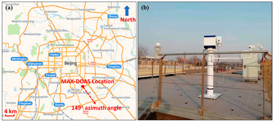
Figure 1.
The location (a) and system characteristics (b) of the multi-axis differential optical absorption spectroscopy (MAX-DOAS) instrument.
2.2. Spectral Analysis
The theoretical basis of MAX-DOAS technology is the Lambert–Beer law [36],
where , , , c, and L represent the radiant light intensity after absorption by atmospheric molecules, the incident light intensity without passing through the atmosphere, the gas absorption cross-section, the gas concentration, and the optical path, respectively. The acquired spectral data were fitted by least squares using QDOAS software (version 3.2, 2017) [37], and the 90° spectrum from the same measurement cycle served as the Fraunhofer reference spectrum (FRS). In the study, the MAX-DOAS system was implemented using a 149° azimuth with a wide field of view to carry out cyclic elevation scanning (facing the South Fifth Ring Road) to avoid occlusion at small elevation angles. The entire elevation angle cycle included 11 elevation angles of 1°, 2°, 3°, 4°, 5°, 6°, 8°, 10°, 20°, 30°, and 90°. Combining the differential slant column density (dSCD) fitted by QDOAS with the air mass factors (AMFs) calculated by the radiative transfer model (RTM, SCAITRAN 2.2) [38], the gas tropospheric vertical column density (VCD) can be obtained as follows [39]:
Table 1 lists the DOAS fitting parameters for the species. Figure 2 shows an example of DOAS fitting for O4, NO2, SO2, and HCHO at 10:06:58 a.m. on 24 April 2020, as well as an example for H2O at 11:51:48 a.m. on 15 May 2020. For the SO2 fitting, only the results with a root-mean-square (RMS) error less than 5 × 10⁻³ were retained, while the results with an RMS less than 1 × 10⁻³ were retained for the other gases. In addition, Lampel et al. (2015) [40] confirmed that the saturated absorption effect of water vapor has a negligible influence on the retrieval results in the 442 nm bandwidth because of relatively weak absorption.

Table 1.
DOAS analysis parameter settings.
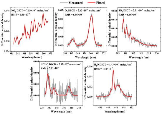
Figure 2.
Examples of typical DOAS fits of O4, NO2, SO2, and HCHO at 10:06:58 a.m. local time (LT) on 24 April 2020, as well as of H2O at 11:51:48 a.m. LT on 15 May 2020.
2.3. Profile Retrieval
The vertical profile retrieval algorithm for aerosol extinction and trace gases (PriAM) used in this study was jointly developed by the AIOFM and Max Planck Institute of Chemistry (MPIC) [29,35,50,51,52]. PriAM is an optimal estimation method, which uses SCIATRAN 2.2 RTM as the forward model (F) to simulate the measurement vector y (M elements) according to the atmospheric state vector x (N elements). Then, the value function is minimized through nonlinear iteration, and the optimal solution is gradually obtained. The expression of the value function is as follows:
where x refers to the vertical profile of aerosol extinction or gases; y refers to the gas at different elevation angles; is the forward model function; , , and represent the a priori state vector, measurement error, and a priori state error, respectively. The subscripts n and m represent the n-th and m-th elements. The iterative process of using the Levenberg–Marquardt algorithm to modify the Gauss–Newton method can be expressed as
where i is the current state, and T represents the transposed matrix. , , and are the measurement error covariance matrix, a priori covariance matrix, and weight function matrix, respectively; is a correction coefficient used to change the rate at which the state quantity approaches the value function. It can be set to 1 and then modified according to the iteration. The generality of the PriAM algorithm for aerosols, NO2, SO2, HCHO, and H2O has been proven in many comparative observation experiments [29,31,32,34,35,50,51,52]. The measurable altitude range for PriAM is 0.05–4 km.
2.4. Transport Flux Calculation
The calculation of water vapor transport flux depends on the water vapor concentration profile calculated by PriAM and the wind profile. The wind profile was measured using the wind profile radar of the Beijing Southern Suburb Observatory with a time resolution of 6 min. In meteorology, the water vapor transport flux is usually divided into zonal and meridional. Therefore, we decomposed the wind into u wind and v wind to calculate the water vapor zonal transport flux (negative indicates transport from east to west, while positive indicates transport from west to east) and meridional transport flux (negative indicates transport from north to south, while positive indicates transport from south to north). The calculation formula for water vapor transport flux of the i-th layer at time t is as follows:
where is the gas concentration (g/m3) corresponding to the height of the i-th layer, and and represent the zonal and meridional transport, respectively. The unit of wind speed is m/s, and the unit of water vapor transport flux in each layer is g/m2/s.
The zonal and meridional water vapor transport fluxes in each layer at time t are superimposed to obtain the vertically integrated water vapor transport fluxes and , respectively.
where is the height resolution of the i-th layer of the flux profile, which is consistent with the resolution of the water vapor profile. The height resolution was 200 m in this study, and the unit of the vertically integrated water vapor transport flux is g/m/s.
3. Results and Discussion
MAX-DOAS observations at the Beijing Southern Suburb Observatory were carried out from 1 January 2020 to 31 December 2020. The aerosol optical depth (AOD), the AE profile, and the VCD and profiles of NO2, SO2, HCHO, and H2O were obtained.
3.1. Annual Observations and Analysis
The monthly distribution of atmospheric pollutants and water vapor in Beijing was analyzed. The monthly averaged results of AOD, H2O VCD, NO2 VCD, SO2 VCD, and HCHO VCD were calculated based on the MAX-DOAS measurements (Figure 3a,b). The monthly mean results of PM2.5 and PM10 from the Yizhuang Air Quality Monitoring Station (116.506°E, 39.795°N) near the MAX-DOAS location are also shown in Figure 3c. Compared to other months, the AOD (retrieved from 360 nm) was larger from May to August (Figure 3a), with a maximum of 0.82 in May. The H2O VCDs were larger from May to September, with a maximum of 1.08 × 10²³ molecules/cm2 in August. The NO2 VCD was relatively high in autumn, with the largest value of 22.21 × 10¹⁵ molecules/cm2 in October. The maximum SO2 VCD, 12.45 × 10¹⁵ molecules/cm2, was recorded in February. HCHO exhibited higher values during summer and lower values during winter, related to the enhanced photochemical reaction during summer.
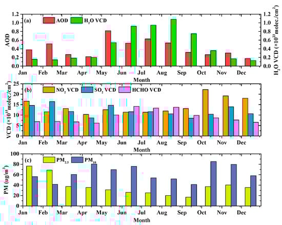
Figure 3.
Monthly distribution characteristics of aerosol and gases: (a) aerosol optical depth (AOD) and H2O vertical column density (VCD); (b) VCDs for NO2, SO2, and HCHO; (c) PM2.5 and PM10.
During autumn and winter, haze pollution events occurred frequently in Beijing, with a higher content of fine particulate matter than in other seasons [18,19]. Figure 3c shows that PM10 pollution was also relatively high during spring (March to June), related to dust transport from the north [20]. We selected the haze and dust pollution periods according to the PM2.5 and PM10 concentrations (Figure 4) and the historical weather patterns to analyze the two typical pollution characteristics. As shown in Figure 4, referring to two specific haze pollution events (from 24 to 29 January 2020 and from 10 to 14 February 2020) and two dust pollution events (18 March 2020 and 24 April 2020) for analysis, it was found that haze pollution mainly manifested as a rise in PM2.5 with a long duration of several days, whereas dust pollution manifested as a sharp rise in PM10 with a short duration of a few hours. These conclusions are as expected due to the mechanical nature of dust formation and the chemical nature of haze formation.
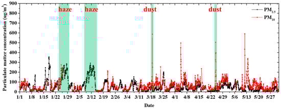
Figure 4.
Hourly variations in PM2.5 and PM10 concentrations from January to May 2020. The pollution events chosen for analysis are shaded in green.
3.2. Analysis of Haze and Dust Pollution Processes
3.2.1. Characteristics of the Correlation between AE and H2O
The level of water vapor concentration affects the processes of haze and dust pollution [18,19,20]. AE is one of the most important aerosol parameters, which characterizes atmospheric turbidity. The correlation between AE and H2O allows for the investigation of its potential impact on haze and dust [53].
The lowest height of the PriAM algorithm retrieved is 50 m, followed by 200 m, and all the layer height resolutions above 200 m, are 200 m. Since pollution often occurs in the near-surface boundary layer, the altitudes of 50 m, 200 m, and 400 m were used to analyze the relationship between H2O mixing ratio (MR) concentration and AE during haze and dust pollution events (Figure 5). To investigate the relationship between H2O MR and AE during the two typical pollution periods, the daily H2O MR (x-axis) and AE (y-axis) were linearly fitted, and the Pearson correlation coefficient (r), as well as the absolute value of the correlation slope (|k|) were calculated (Figure 5). The two haze pollution events from 24 to 29 January and from 10 to 14 February are labeled Haze 1 and Haze 2, respectively, while the two dust pollution events on 18 March and on 24 April are labeled Dust 1 and Dust 2, respectively.
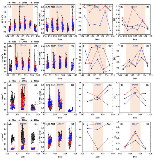
Figure 5.
The relationship between H2O MR and AE at heights of 50 m, 200 m, and 400 m during the haze and dust pollution events. (a–d), (e–h), (i–l), and (m–p) represent the Haze 1, Haze 2, Dust 1, and Dust 2 pollution events, respectively. Days with serious pollution are shaded in red.
Figure 5 shows that the AE at 50 m was significantly higher than that at 200 m and 400 m during the dust pollution events. During the haze pollution events, the AE also decreased with the height, but this trend was more obvious for dust pollution (Figure 5i,m). The AE and H2O MR showed the same trend during both haze pollution events, i.e., a slowly increasing trend before decreasing. During the dust pollution events, r decreased and |k| increased, whereas r increased and |k| decreased during the haze pollution events (Figure 5). Therefore, the O4 absorption was enhanced during the dust period, while the H2O absorption increased significantly during the haze period. In addition, the values of r at 50 m were close to 1 and 0.8 (Figure 5c,g) for Haze 1 and Haze 2, respectively, which indicates that the secondary aerosol formation is affected by water vapor during the haze pollution process, mainly occurring around or below 50 m. The variations in the correlation between AE and H2O MR can help us understand the occurrence of haze and dust.
3.2.2. The Variations in Gas VCD and Meteorological Factors
The variations in AOD, NO2 VCD, SO2 VCD, HCHO VCD, and H2O VCD during haze and dust pollution were analyzed, and the results are presented in Figure 6 and Figure 7. To analyze the impact of meteorological factors on the pollution process, we also conducted a statistical analysis of hourly near-ground meteorological data at the Beijing Southern Suburb Observatory (Figure 8).
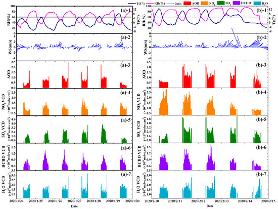
Figure 6.
Variations in gas VCDs during the process of haze pollution. (a,b) represent Haze 1 and Haze 2. 1 to 7 represent RH, WS, AOD, NO2 VCD, SO2 VCD, HCHO VCD, and H2O VCD, respectively.
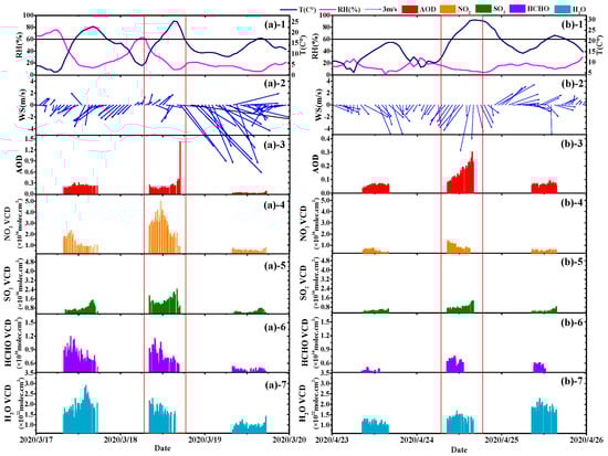
Figure 7.
Variations in gas VCDs during the process of dust pollution. (a,b) represent Dust 1 and Dust 2. 1 to 7 represent RH, WS, AOD, NO2 VCD, SO2 VCD, HCHO VCD, and H2O VCD, respectively. The two red boxes in the figure represent the dusty days.
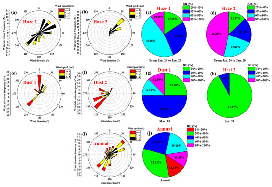
Figure 8.
Statistics related to wind and relative humidity during the pollution processes. (a,b) represent the wind field during the haze pollution periods; (c,d) represent the RH during the haze pollution periods; (e,f) represent the wind field during the dust pollution periods; (g,h) represent the RH during the dust pollution periods; (i,j) respectively represent the wind field and RH during the observation period (one year).
Figure 6(a-3,b-3) and Figure 7(a-3,b-3) show that AOD was high in the morning and evening and low at noon during these two haze pollution periods, while the AOD increased during these two dust pollution periods in the afternoon, and the water vapor concentration decreased. During these two haze pollution periods, SO2 and HCHO VCD showed a trend of first increasing and then decreasing. The biggest difference between haze and dust pollution was represented by the different meteorological conditions (Figure 6(a-1,a-2,b-1,b-2) and Figure 7(a-1,a-2,b-1,b-2)), which is similar to previous studies [11,12,13,20,21]. The annual meteorological conditions are shown in Figure 8i,j. The annual average wind speed was 2.66 m/s, and the wind directions were mainly concentrated in the northeast (45° and 70°) and southwest (200° and 215°). The annual RH was concentrated between 20% and 60%. The near-surface wind speeds during haze pollution were lower than the annual average wind speed, and they were basically less than 2 m/s (Figure 8a,b). These two haze pollution events with RH higher than 60% accounted for 56.46% and 69.01%, respectively (Figure 8c,d), indicating that the aerosol particles contain a large quantity of water [54]. Moreover, the low wind speeds and southeast air were unfavorable for diffusion conditions, leading to continuous haze pollution. The wind speeds were relatively higher (mostly greater than 4 m/s) than the annual average wind speed and mainly from the northwest direction during dust pollution events (Figure 8e,f). Most of the RH was <60% during dust pollution (Figure 8g,h).
To further analyze the meteorological conditions in large regions, the European Centre for Medium-Range Weather Forecasts (ECMWF) (https://cds.climate.copernicus.eu accessed on 20 October 2021) ERA5 climate reanalysis data were used to analyze the regional distribution of wind vectors and RH for the two haze and dust pollution events, as shown in Figures S1 and S2 in the supplement. ERA5 is ECMWF’s latest climate reanalysis product, providing hourly data on various atmospheric, surface, and ocean parameters. Figures S1 and S2 show the wind vectors and RH near the ground (120 m) at 12:00 LT during the haze and dust pollution periods, respectively. During the period of haze pollution (Figure S1), Beijing appeared to have static stability and high-humidity weather conditions. There are high humidity air masses in the ocean southeast of Beijing. The northeasterly wind was blowing in the upper part of the ocean, leading to the easterly wind bringing the moisture mass to Beijing, and thus exacerbating the haze pollution. The northwest wind in Beijing was dominant and the wind speeds were relatively higher during dust pollution periods (Figure S2). RH in regions such as Inner Mongolia in the northwest were less than 30%. We also downloaded PM10 data at 8:00 LT from the ECMWF CAMS global atmospheric composition forecasts model (see Figure S3 in the supplement). The CAMS model contains various atmospheric composition data at 0:00 and 12:00 UTC. It can be found that the PM10 concentration was higher in Mongolia on dusty days (18 March and 24 April). As there are many deserts in Mongolia, the dry air masses from the northwest bring a large amount of sand and dust to Beijing.
The mean value of AOD (retrieved from 360 nm) during haze pollution (AOD = 0.66) was significantly greater than that during dust pollution (AOD = 0.13). This is mainly because the AOD at 360 nm reflects the concentration of fine particles. Haze pollution mainly involves fine particles, whereas dust pollution mainly involves coarse particles. During the Haze 2 event, the NO2 VCD was relatively high when pollution occurred. As the AOD increased, the NO2 VCD decreased significantly (Figure 6(b-4)), which may be related to the liquid-phase reaction [54]. NO2 is converted to nitrate in the liquid-phase reaction, thereby enhancing the formation of secondary aerosols and further leading to a rapid increase in aerosol concentration [19]. SO2 showed no obvious decreasing trend during Haze 2 (Figure 6(b-5)); thus, the aerosol concentration was mainly contributed by the liquid-phase reaction of nitrogen oxides. Beijing is a typical megacity, with a large population and a corresponding number of petrol (gasoline) powered vehicles. Because there are no large-scale chemical plants nearby, nitrogen oxide emitted by vehicles represents the main source of pollution in Beijing [55]. Since fireworks and firecrackers are banned in Beijing, the increase in SO2 concentration during both haze pollution events may have been related to the display of fireworks and firecrackers in the cities surrounding Beijing (25 January is the Chinese New Year and 8 February is the Lantern Festival).
3.2.3. The Gas Vertical Distribution
The vertical profiles of AE, NO2, SO2, HCHO, and H2O during the haze and dust pollution periods are shown in Figure 9 and Figure 10.
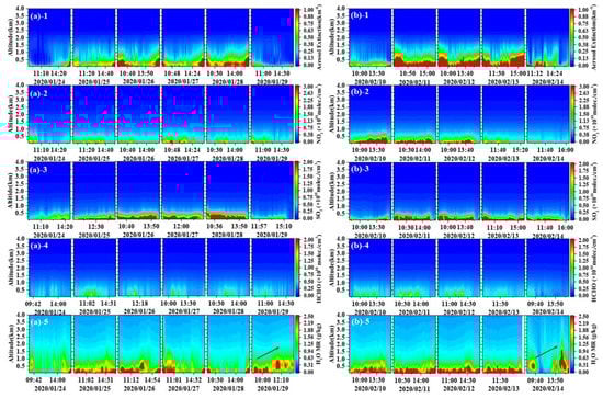
Figure 9.
Variations in gas profiles during the haze pollution events. (a,b) represent Haze 1 and Haze 2. Numbers 1 to 5 represent aerosol extinction (AE), NO2, SO2, HCHO, and H2O mixing ratio concentration, respectively. The two red arrows in the figure indicate the increase in H2O concentration.
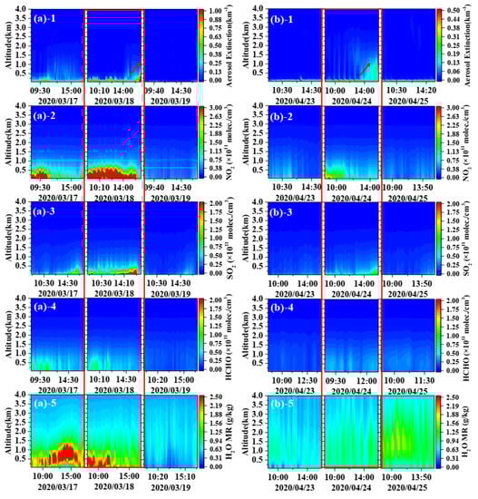
Figure 10.
Variations in gas profiles during the dust pollution events. (a,b) represent Dust 1 and Dust 2. Numbers 1 to 5 represent aerosol extinction (AE), NO2, SO2, HCHO, and H2O mixing ratio concentration, respectively. The two red boxes represent the dusty days in the figure, and the two red arrows indicate the increase in AE.
Figure 9 shows that both haze pollution events were dominated by SO2 and NO2 pollution, whereas the concentration of HCHO was lower. The aerosols were mainly concentrated below 1.0 km, and the near-ground AE ranged from 0.18 to 2.68 km−1 during haze pollution, showing a trend of being high in the morning and evening but low at noon. NO2, SO2, HCHO, and H2O were all concentrated below 0.5 km during haze pollution, which promoted the transformation of gaseous pollutants to secondary aerosol components. Aerosols and SO2 exhibited the same accumulation and dissipation process during haze pollution. During Haze 2, NO2 was already at a high concentration when the pollution started on 10 February. As the pollution level worsened, NO2 decreased from 11 to 14 February (Figure 9(b-2)), while the NO2 VCDs also showed a similar trend (Figure 6(b-4)), which may have been related to the liquid-phase reaction of NO2 [54].
The two dust pollution events showed a sharp increase in AE over a short time, and the pollution height reached 1.0 km (see the red box in Figure 10(a-1,b-1)). Compared with the haze pollution periods, the near-ground aerosol extinction coefficients were smaller (0.10 to 0.84 km−1) on dusty days, in line with the results of previous reports [56]. The dust pollution lasted for a short time, and the aerosol extinction coefficient dropped within a few hours. Due to the light intensity demands of MAX-DOAS, the nighttime dissipation processes of the two dust pollution events were not captured. The morning after the dust pollution, the dust had dissipated (see the AE on 19 March and 25 April in Figure 10). NO2, SO2, and HCHO were all concentrated below 0.5 km during dust pollution, as also observed for haze pollution.
We then analyzed the sounding profiles for temperature and water vapor at the Beijing Southern Suburb Observatory. There were two sounding profiles recorded for temperature and water vapor each day, at around 11:00 a.m. and 11:00 p.m. local time. Due to the limited measuring time of MAX-DOAS, the morning sounding profile was used for analysis every day (Figure 11 and Figure 12).
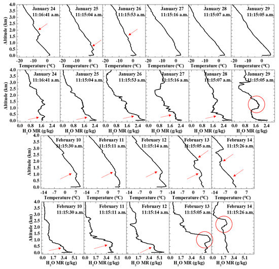
Figure 11.
The sounding profiles (temperature and water vapor mixing ratio) during haze pollution. The red arrow represents the area of large variation, and the red circle represents the area where the H2O mixing ratio concentration rises.
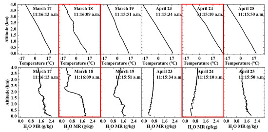
Figure 12.
The sounding profiles (temperature and water vapor mixing ratio) during dust pollution. The two red boxes represent the dusty days in the figure.
The sounding profiles for temperature during the haze pollution periods show that a strong temperature inversion occurred in the vertical direction, and the temperature inversion intensity reached its peak at about 1.0 km (Figure 11), limiting the diffusion of pollutants. Additionally, it appears from this data that high humidity in the lower atmosphere was required to promote the early stages of haze formation. When the haze dissipated, water vapor was transported upward from the near-surface, as seen in the MAX-DOAS observations (Figure 9(a-5,b-5)). The high concentration of water vapor near the ground spread to the upper air when the pollution dissipated, thereby alleviating the high near-surface humidity. Therefore, the accumulation of water vapor near the ground during haze pollution is conducive to the formation of haze.
Figure 12 indicates that there was no temperature inversion during the dust pollution process, and water vapor did not gather near the ground. On 24 April, the water vapor concentration even recorded its lowest value at the near-surface.
About 120 km southeast of Beijing is the Bohai Sea, and the high-humidity air mass over the ocean may affect the humidity in Beijing. The increase of water vapor concentration is conducive to the formation of haze. Therefore, it is of significance to study water vapor transport during haze pollution events.
We calculated the water vapor transport flux during the two haze pollution events according to the method described in Section 2.4. Since Beijing has many tall buildings, the direction of transport flux within 0.2 km of the ground is easily affected. Therefore, the zonal (east–west) and meridional (north–south) water vapor transport from 0.2 km to 3.8 km was analyzed (Figure 13).
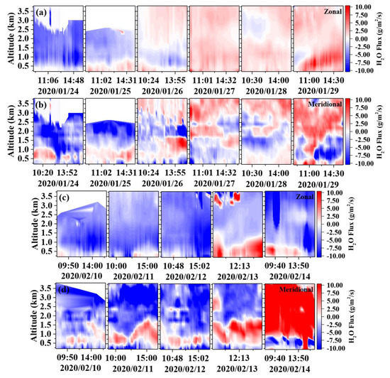
Figure 13.
The zonal and meridional H2O transport fluxes during haze pollution: (a) zonal H2O transport fluxes during Haze 1; (b) meridional H2O transport fluxes during Haze 1; (c) zonal H2O transport fluxes during Haze 2; (d) meridional H2O transport fluxes during Haze 2.
The flux results indicate that the meridional water vapor transport occurred from south to north in the vicinity of 0.4 km to 1.0 km during both haze pollution events (Figure 13b,d), whereas it was mainly transported from north to south at altitudes above 1.2 km.
The zonal water vapor transport flux mainly occurred from east to west during Haze 2 pollution event, and this was also the case for Haze 1 in the first 3 days (Figure 13a,c). Therefore, the occurrence of haze pollution is closely related to water vapor transport from the east.
Figure 14 shows the total zonal and meridional water vapor transport fluxes during both haze pollution events. The zonal water vapor transport flux generally occurred from east to west (negative), and it was mainly distributed at around 1.0 km. The maximum zonal transport height was 1.0 km during Haze 2, with a corresponding transport flux of −1526.92 g/m2/s. In general, the meridional water vapor transport flux occurred from north to south (negative), and it was mainly distributed at about 0.2 km, 2.0 km, and 3.0 km. The maximum meridional transport height was 3.2 km during Haze 2, with a corresponding transport flux of −1755.75 g/m2/s.
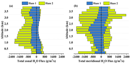
Figure 14.
The zonal (a) and meridional (b) H2O transport fluxes during haze pollution.
The vertically integrated water vapor transport fluxes from 0.2 km to 3.8 km were calculated during the haze pollution events using Equation (6) with a vertical resolution of 200 m. The results indicate that the total vertically integrated water vapor transport flux, with a value of 5287.06 kg/m/s from east to west, was about 3.88 times that from west to east (Table 2). The total vertically integrated water vapor transport flux from north to south, with a value of 6285.60 kg/m/s, was about 1.66 times that from south to north (Table 2). Therefore, the water vapor transport from the eastern air mass had an auxiliary effect on haze pollution at the observation sites. This is related to the high-humidity air masses in the ocean southeast of Beijing (see Figure S1 in the supplement).
Table 2.
The vertically integrated H2O transport flux during haze pollution.
4. Discussions
4.1. Cluster Analysis of Air Mass Back Trajectories
Figure 15 shows the cluster analysis of 24-h air mass back trajectories at 0.5 km and 1.0 km during the haze and dust pollution periods. The dust pollution period mainly featured air mass transmission from the northwest (Mongolia direction), and the wind speeds were relatively high (Figure 15e–h). As there are many deserts with wind erosion potential in Mongolia, the back trajectories of these dust incidents indicate a potential transport for a long travel distance. However, there are also construction sites along with the wind back trajectories, possibly mineral processing locations, or road works nearby the sampling location, which all bring sand and dust to Beijing. On the other hand, it mainly featured local transportation from the southeast during the haze pollution period, and the wind speeds were relatively low (Figure 15a–d).
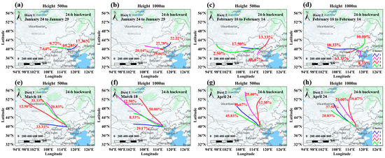
Figure 15.
The cluster analysis of 24-h air mass backward trajectories of the (a–d) haze and (e–h) dust cases at heights of 0.5 km and 1.0 km.
4.2. Source Identification of the Pollutions
To analyze the pollution transport and potential source regions of aerosol in Beijing, we used the Potential Source Contribution Function (PSCF) and the Concentration-Weighted Trajectory (CWT) model to evaluate the lower boundary layer and the upper boundary layer [57,58,59]. The PSCF is based on the backward trajectory space grid to calculate the probability of the polluted trajectory endpoint number in each grid. The CWT analyzes its pollution contribution to the target grid by calculating the average weight concentration of the source grid. Regional atmospheric transport can be better understood by studying potential pollution sources at different altitudes.
In this paper, the study domain was divided into 0.5° × 0.5° grid cells. Hourly aerosol extinction coefficient from MAX-DOAS measurement joined with corresponding 72 h back trajectories in the lower (200 m) and upper (1000 m) altitudes were used as input for the PSCF and CWT model. Figure 16 and Figure 17 show the weighted calculation results of PSCF and CWT (WPSCF and WCWT) of the trajectory grids for the months with frequent haze pollution (January and February) and dust pollution (March, April, and May) in Beijing. In general, the potential aerosol source regions at higher altitudes were more widespread than the source regions at lower altitudes. In January and February, the most potential source areas with WPSCF values for aerosol were from Shandong in the south and Inner Mongolia in the northwest of Beijing (Figure 16). The WCWT values show that the transported aerosols at lower altitudes from the northwest areas made a significant contribution to aerosols in Beijing. In March, April, and May, the greatest potential sources with WPSCF values for aerosol were from Shandong, Henan, and other places in the south of Beijing (Figure 17). The WCWT values show that the transported aerosols at lower altitudes from the southern region made a great contribution to Beijing.
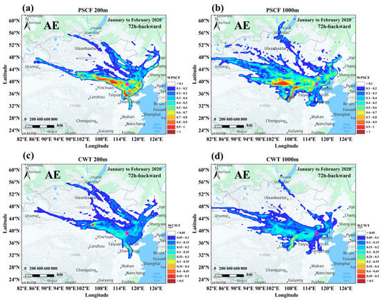
Figure 16.
Spatial distributions of WPSCF (a,b) and WCWT (c,d) values for aerosol extinction coefficient at 200 m (left panel) and 1000 m (right panel) altitudes in January and February 2020 over Beijing. The purple five-pointed star symbol represents Beijing.
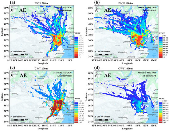
Figure 17.
Spatial distributions of WPSCF (a,b) and WCWT (c,d) values for aerosol extinction coefficient at 200 m (left panel) and 1000 m (right panel) altitudes in March, April, and May 2020 over Beijing. The purple five-pointed star symbol represents Beijing.
In addition, hourly PM2.5 and PM10 data from near-surface measurements joined with corresponding 72 h back trajectories in the lower (200 m) were used as input for the PSCF model (Figure 18). The WPSCF values of the aerosol extinction coefficient (retrieved at 360 nm) were similar to that of PM2.5 at 200 m. The potential source regions of PM2.5 in January and February were more widespread than the source regions from March to May, while PM10 is the opposite. This is related to the seasonal pollution characteristics in Beijing. In January and February, the most potential source areas with WPSCF values for PM2.5 were from the surrounding areas of Beijing and Inner Mongolia in the northwest of Beijing (Figure 18a). The most potential source areas with WPSCF values for PM10 were from Henan in the south and Inner Mongolia in the northwest of Beijing (Figure 18d).
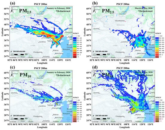
Figure 18.
Spatial distributions of WPSCF values for PM2.5 (a,b) and PM10 (c,d) at 200 m altitude from January to May 2020 in Beijing. The purple five-pointed star symbol represents Beijing.
5. Conclusions
Haze and dust pollution have attracted widespread attention due to their notable impact on human health and productivity. This study carried out one-year observations (from 1 January 2020 to 31 December 2020) at the Beijing Southern Suburb Observatory using MAX-DOAS and analyzed the characteristics of pollutant gases and meteorological factors during the two typical processes of haze and dust. Two haze and dust pollution events were selected for this study.
Firstly, the variations in aerosol and water vapor concentration during haze and dust pollution at different heights were analyzed. The linear fitting results of the H2O mixing ratio concentration and AE indicated that the correlation coefficient (r) decreased and the correlation slope (|k|) increased during dust pollution, whereas the r increased and |k| decreased during haze pollution. Therefore, the O4 absorption was enhanced during the dust period, while the H2O absorption increased significantly during the haze period.
Secondly, the gas vertical column density and near-surface meteorological conditions during the two typical pollution events were analyzed. The AOD was high in the morning and evening and low at noon during the two haze pollution periods, while the AOD increased in the afternoon during the two dust pollution events, and the H2O concentration decreased. This same trend of AOD, SO2 VCD and HCHO VCD was observed during haze pollution (slowly increasing before decreasing), while SO2 VCD and HCHO VCD show no obvious regular changes during dust pollution. There are high-humidity air masses in the ocean southeast of Beijing during haze pollution periods. The northeasterly wind was blowing in the upper part of the ocean, which led to the easterly wind bringing the moisture mass to Beijing and thus exacerbating the haze pollution. During dust pollution days, the dry air masses from the northwest (Mongolia) bring a large amount of sand and dust to Beijing.
Thirdly, we studied the vertical distribution of gases during the pollution period. Aerosols and H2O were concentrated below 1.0 km, with the aerosols tending to be high in the morning and evening and lower at noon during haze pollution. Aerosols and SO2 exhibited the same accumulation and dissipation process during haze pollution. During dust pollution, the aerosol extinction coefficient quickly increased over a short time, and the pollution altitude reached 1.0 km. In addition, high PM10 and PM2.5 dust levels dropped within a few hours of the dust pollution starting. NO2, SO2, and HCHO were all concentrated below 0.5 km during both typical pollution processes. The temperature and humidity sounding profiles showed that haze pollution formation is associated with a strong temperature inversion at around 1.0 km; furthermore, high humidity in the lower atmosphere was required to promote the early stages of the haze formation.
Next, we studied the transportation of water vapor during haze pollution. The zonal water vapor transport was the largest at about 1.0 km, whereas the meridional transport was higher at about 0.2 km, 2.0 km, and 3.0 km. The flux of water vapor transport from east to west was about 3.88 times that from west to east, whereas the flux of water vapor transport from north to south was about 1.66 times that from south to north. This indicates that water vapor from the east has an auxiliary effect on haze pollution of the observation location. This is related to the high-humidity air masses in the ocean southeast of Beijing.
Lastly, the 24-h air mass backward trajectories indicated that the dust pollution was mainly due to the transmission of air mass from the northwest, with a relatively high wind speed. On the other hand, haze pollution was mainly due to local transportation from the southeast, accompanied by lower wind speeds.
Our study illustrated the spatiotemporal differences between haze and dust pollution incidents and reflects the application value of MAX-DOAS remote sensing instruments.
Supplementary Materials
The following are available online at https://www.mdpi.com/article/10.3390/rs13245133/s1, Figure S1: The regional distribution of wind vectors (a) and RH (b) from ERA5 climate reanalysis data during haze pollution periods. 1 to 11 represent different dates. The red dots represent Beijing, Figure S2: The regional distribution of wind vectors (a) and RH (b) from ERA5 climate reanalysis data during dust pollution periods. 1 to 6 represent different dates. The red dots represent Beijing. The two red boxes represent the dusty days in the figure, Figure S3: The regional distribution of PM10 from the CAMS model on dusty days (March 18 and April 24). (a) March 18; (b) April 24. The red dots represent Beijing.
Author Contributions
H.R., A.L. and Z.H. designed the experiments. H.R., Y.H. and X.L. performed the MAX-DOAS experiment and processed the MAX-DOAS data. X.T., B.R., S.W., W.C. and H.Z. (Hongyan Zhong) helped process meteorological data. H.R., C.D. and H.Z. (Hairong Zhang) processed the wind profile data. P.X. and J.X. supervised this study. H.R. analyzed the data and wrote the paper. All authors have read and agreed to the published version of the manuscript.
Funding
This work was supported by the National Natural Science Foundation of China (No.: 41775029, 41975037), the National Key Research and Development Project of China (No.: 2018YFC0213201, 2018YFC0213801), the Science and Technology Commission of Shanghai Municipality (No.: 17DZ1203102), and Key Research and Development Project of Anhui Province (No.: 202004i07020013).
Data Availability Statement
The data are available upon request by email to Hongmei Ren at hmren@aiofm.ac.cn.
Acknowledgments
We thank the Belgian Institute for Space Aeronomy (BIRAIASB), Brussels, Belgium, for their freely accessible QDOAS software. We also thank the National Oceanic and Atmospheric Administration (NOAA) Air Resources Laboratory (ARL) for the provision of the HYSPLIT transport and dispersion model used in this publication.
Conflicts of Interest
The authors declare no conflict of interest.
References
- Ding, Y.H.; Liu, Y.J. Analysis of long-term variations of fog and haze in China in recent 50 years and their relations with atmospheric humidity. Sci. China Earth Sci. 2014, 57, 36–46. [Google Scholar] [CrossRef]
- Huang, R.J.; Zhang, Y.; Bozzetti, C.; Ho, K.F.; Cao, J.J.; Han, Y.; Daellenbach, K.R.; Slowik, J.G.; Platt, S.M.; Canonaco, F.; et al. High secondary aerosol contribution to particulate pollution during haze events in China. Nature 2014, 7521, 218–222. [Google Scholar] [CrossRef] [PubMed] [Green Version]
- Pei, L.; Yan, Z.; Chen, D.; Miao, S. Climate variability or anthropogenic emissions: Which caused Beijing Haze? Environ. Res. Lett. 2020, 15, 034004. [Google Scholar] [CrossRef]
- Wei, W.; Li, Y.; Wang, Y.; Cheng, S.; Wang, L. Characteristics of VOCs during haze and non-haze days in Beijing, China: Concentration, chemical degradation and regional transport impact. Atmos. Environ. 2018, 194, 134–145. [Google Scholar] [CrossRef]
- Zhang, R.; Sun, X.; Shi, A.; Huang, Y.; Yan, J.; Nie, T.; Yan, X.; Li, X. Secondary inorganic aerosols formation during haze episodes at an urban site in Beijing, China. Atmos. Environ. 2018, 177, 275–282. [Google Scholar] [CrossRef]
- Li, W.; Liu, X.; Zhang, Y.; Tan, Q.; Feng, M.; Song, M.; Hui, L.; Qu, Y.; An, J.; Gao, H. Insights into the phenomenon of an explosive growth and sharp decline in haze: A case study in Beijing. J. Environ. Sci. 2019, 84, 122–132. [Google Scholar] [CrossRef] [PubMed]
- Zhang, Q.; Jiang, X.; Tong, D.; Davis, S.; Zhao, H.; Geng, G. Transboundary health impacts of transported global air pollution and international trade. Nature 2017, 543, 705–709. [Google Scholar] [CrossRef] [Green Version]
- Lolli, S.; Chen, Y.-C.; Wang, S.-H.; Vivone, G. Impact of meteorological conditions and air pollution on COVID-19 pandemic transmission in Italy. Sci. Rep. 2020, 10, 16213. [Google Scholar] [CrossRef]
- Wu, X.; Nethery, R.C.; Sabath, M.B.; Braun, D.; Dominici, F. Exposure to air pollution and COVID-19 mortality in the United States: A nationwide cross-sectional study. medRxiv 2020. [Google Scholar] [CrossRef] [Green Version]
- Lian, X.; Huang, J.; Huang, R.; Liu, C.; Wang, L.; Zhang, T. Impact of city lockdown on the air quality of COVID-19-hit of Wuhan city. Sci. Total Environ. 2020, 742, 140556. [Google Scholar] [CrossRef]
- Flocas, H.; Kelessis, A.; Helmis, C.; Petrakakis, M.; Zoumakis, M.; Pappas, K. Synoptic and local scale atmospheric circulation associated with air pollution episodes in an urban Mediterranean area. Theor. Appl. Climatol. 2009, 95, 265–277. [Google Scholar] [CrossRef]
- Quan, J.; Yang, G.; Qiang, Z.; Tie, X.; Cao, J.; Han, S.; Meng, J. Evolution of planetary boundary layer under different weather conditions, and its impact on aerosol concentrations. Particuology 2013, 11, 34–40. [Google Scholar] [CrossRef]
- Zhang, R.H.; Qiang, L.I.; Zhang, R.N. Meteorological conditions for the persistent severe fog and haze event over eastern China in January 2013. Sci. China Earth Sci. 2014, 54, 26–35. [Google Scholar]
- Wagner, T.; Andreae, M.O.; Beirle, S.; Doerner, S.; Mies, K.; Shaiganfar, R. MAX-DOAS observations of the total atmospheric water vapour column and comparison with independent observations. Atmos. Meas. Tech. 2013, 6, 131–149. [Google Scholar] [CrossRef] [Green Version]
- Ryu, Y.H.; Smith, J.A.; Bou-Zeid, E. On the Climatology of Precipitable Water and Water Vapor Flux in the Mid-Atlantic Region of the United States. J. Hydrometeorol. 2014, 16, 70–87. [Google Scholar] [CrossRef]
- Wu, J.; Bei, N.; Hu, B.; Liu, S.; Zhou, M.; Wang, Q.; Li, X.; Liu, L.; Feng, T.; Liu, Z.; et al. Is water vapor a key player of the wintertime haze in North China Plain? Atmos. Chem. Phys. 2019, 19, 8721–8739. [Google Scholar] [CrossRef] [Green Version]
- Wang, J.Z.; Wang, Y.Q.; Liu, H.; Yang, Y.Q.; Zhang, X.Y.; Li, Y.; Zhang, Y.M.; Deng, G. Diagnostic Identification of the Impact of Meteorological Conditions on PM2.5 Concentration in Beijing. Atmos. Environ. 2013, 81, 158–165. [Google Scholar] [CrossRef]
- Wu, P.; Ding, Y.; Liu, Y. Atmospheric circulation and dynamic mechanism for persistent haze events in the Beijing–Tianjin–Hebei region. Adv. Atmos. Sci. 2017, 34, 429–440. [Google Scholar] [CrossRef] [Green Version]
- Liu, Y.; Wu, Z.; Huang, X.; Shen, H.; Bai, Y.; Qiao, K.; Meng, X.; Hu, W.; Tang, M.; He, L. Aerosol Phase State and Its Link to Chemical Composition and Liquid Water Content in a Subtropical Coastal Megacity. Environ. Sci. Technol. 2019, 53, 5027–5033. [Google Scholar] [CrossRef]
- Tong, L.; Zhao, H. Analysis on the Gale and Dust Weather in Zhangjiakou City on 11 May 2011. Meteorol. Environ. Res. 2018, 9, 5–10. [Google Scholar]
- Chen, H.; Zhao, L.; Zhao, L.; Tian, H.; Wu, H.; Xun, N. Effects of sand dust weather on the air quality of Beijing. Res. Environ. Sci. 2012, 25, 609–614. [Google Scholar]
- Hansell, R.A.; Tsay, S.C.; Hsu, N.C.; Qiang, J.; Bell, S.W.; Holben, B.N.; Welton, E.J.; Roush, T.L.; Zhang, W.; Huang, J. An assessment of the surface longwave direct radiative effect of airborne dust in Zhangye, China, during the Asian Monsoon Years field experiment (2008). J. Geophys. Res. Atmos. 2012, 117, D00K39. [Google Scholar] [CrossRef] [Green Version]
- Zhou, M.; Chen, C.; Wang, H.; Huang, C.; Su, L.; Chen, Y.; Li, L.; Qiao, Y.; Chen, M.; Huang, H.; et al. Chemical characteristics of particulate matters during air pollution episodes in autumn of Shanghai, China. Acta Sci. Circumstantiae 2012, 32, 81–92. [Google Scholar]
- Pachauri, T.; Singla, V.; Satsangi, A.; Lakhani, A.; Kumari, K.M. Characterization of major pollution events (dust, haze, and two festival events) at Agra, India. Environ. Sci. Pollut. Res. 2013, 20, 5737–5752. [Google Scholar] [CrossRef]
- Huang, X.; Zhang, J.; Luo, B.; Wang, L.; Tang, G.; Liu, Z.; Song, H.; Zhang, W.; Yuan, L.; Wang, Y. Water-soluble ions in PM2.5 during spring haze and dust periods in Chengdu, China: Variations, nitrate formation and potential source areas. Environ. Pollut. 2018, 243, 1740–1749. [Google Scholar] [CrossRef]
- Honninger, G.; Friedeburg, C.V.; Platt, U. Multi axis differential optical absorption spectroscopy (MAX-DOAS). Atmos. Chem. Phys. 2004, 4, 231–254. [Google Scholar] [CrossRef] [Green Version]
- Irie, H.; Takashima, H.; Kanaya, Y.; Boersma, K.F.; Gast, L.; Wittrock, F.; Brunner, D.; Zhou, Y.; Van Roozendael, M. Eight-component retrievals from ground-based MAX-DOAS observations. Atmos. Meas. Tech. 2011, 4, 1027–1044. [Google Scholar] [CrossRef] [Green Version]
- Wang, Y.; Beirle, S.; Hendrick, F.; Hilboll, A.; Jin, J.; Kyuberis, A.A.; Lampel, J.; Li, A.; Luo, Y.; Lodi, L.; et al. MAX-DOAS measurements of HONO slant column densities during the MAD-CAT campaign: Inter-comparison, sensitivity studies on spectral analysis settings, and error budget. Atmos. Meas. Tech. 2017, 10, 3719–3742. [Google Scholar] [CrossRef] [Green Version]
- Tian, X.; Xie, P.; Xu, J.; Li, A.; Wang, Y.; Qin, M.; Hu, Z. Long-term observations of tropospheric NO2, SO2 and HCHO by MAX-DOAS in Yangtze River Delta area, China. J. Environ. Sci. 2018, 71, 207–221. [Google Scholar] [CrossRef] [PubMed]
- Wang, Y.; Doerner, S.; Donner, S.; Boehnke, S.; De Smedt, I.; Dickerson, R.R.; Dong, Z.; He, H.; Li, Z.; Li, Z.; et al. Vertical profiles of NO2, SO2, HONO, HCHO, CHOCHO and aerosols derived from MAX-DOAS measurements at a rural site in the central western North China Plain and their relation to emission sources and effects of regional transport. Atmos. Chem. Phys. 2019, 19, 5417–5449. [Google Scholar] [CrossRef] [Green Version]
- Li, X.; Xie, P.; Li, A.; Xu, J.; Hu, Z. Variation Characteristics and Transportation of Aerosol, NO2, SO2, and HCHO in Coastal Cities of Eastern China: Dalian, Qingdao, and Shanghai. Remote Sens. 2021, 13, 892. [Google Scholar] [CrossRef]
- Ren, H.-M.; Li, A.; Hu, Z.-K.; Huang, Y.-Y.; Xu, J.; Xie, P.-H.; Zhong, H.-Y.; Li, X.-M. Measurement of atmospheric water vapor vertical column concentration and vertical distribution in Qingdao using multi-axis differential optical absorption spectroscopy. Acta Phys. Sin. 2020, 69, 204204. [Google Scholar] [CrossRef]
- Lin, H.; Liu, C.; Xing, C.; Hu, Q.; Hong, Q.; Liu, H.; Li, Q.; Tan, W.; Ji, X.; Wang, Z.; et al. Validation of Water Vapor Vertical Distributions Retrieved from MAX-DOAS over Beijing, China. Remote Sens. 2020, 12, 3193. [Google Scholar] [CrossRef]
- Ren, H.; Li, A.; Xie, P.; Hu, Z.; Zhang, H. Estimation of the Precipitable Water and Water Vapor Fluxes in the Coastal and Inland Cities of China Using MAX-DOAS. Remote Sens. 2021, 13, 1675. [Google Scholar] [CrossRef]
- Wang, Y.; Lampel, J.; Xie, P.; Beirle, S.; Li, A.; Wu, D.; Wagner, T. Ground-based MAX-DOAS observations of tropospheric aerosols, NO2, SO2 and HCHO in Wuxi, China, from 2011 to 2014. Atmos. Chem. Phys. 2017, 17, 2189–2215. [Google Scholar] [CrossRef] [Green Version]
- Platt, U.; Stutz, J. Differential Optical Absorption Spectroscopy; Springer: Heidelberg/Berlin, Germany, 2008. [Google Scholar]
- Danckaert, T.; Fayt, C.; Van Roozendael, M.; De Smedt, I.; Letocart, V.; Merlaud, A.; Pinardi, G. QDOAS Software User Manual Version 3.2. 2017. Available online: https://uv-vis.aeronomie.be/software/QDOAS/QDOAS_manual.pdf (accessed on 20 October 2021).
- Rozanov, V.V.; Rozanov, A.V.; Kokhanovsky, A.A.; Burrows, J.P. Radiative transfer through terrestrial atmosphere and ocean: Software package SCIATRAN. J. Quant. Spectrosc. Radiat. Transf. 2014, 133, 13–71. [Google Scholar] [CrossRef]
- Ibrahim, O.; Platt, U.; Shaiganfar, R.; Wagner, T. Mobile MAX-DOAS observations of tropospheric trace gases. Atmos. Meas. Tech. 2010, 3, 129–140. [Google Scholar]
- Lampel, J.; Poehler, D.; Tschritter, J.; Friess, U.; Platt, U. On the relative absorption strengths of water vapour in the blue wavelength range. Atmos. Meas. Tech. 2015, 8, 4329–4346. [Google Scholar] [CrossRef] [Green Version]
- Vandaele, A.C.; Hermans, C.; Simon, P.C.; Carleer, M.; Colin, R.; Fally, S.; Merienne, M.F.; Jenouvrier, A.; Coquart, B. Measurements of the NO2 absorption cross-section from 42,000 cm−1 to 10,000 cm−1 (238–1000 nm) at 220 K and 294 K. J. Quant. Spectrosc. Radiat. Transf. 1998, 59, 171–184. [Google Scholar] [CrossRef] [Green Version]
- Serdyuchenko, A.; Gorshelev, V.; Weber, M.; Chehade, W.; Burrows, J.P. High spectral resolution ozone absorption cross-sections—Part 2: Temperature dependence. Atmos. Meas. Tech. 2014, 7, 625–636. [Google Scholar] [CrossRef] [Green Version]
- Thalman, R.; Volkamer, R. Temperature dependent absorption cross-sections of O2-O2 collision pairs between 340 and 630 nm and at atmospherically relevant pressure. Phys. Chem. Chem. Phys. 2013, 15, 15371–15381. [Google Scholar] [CrossRef]
- Bogumil, K.; Orphal, J.; Homann, T.; Voigt, S.; Spietz, P.; Fleischmann, O.C.; Vogel, A.; Hartmann, M.; Kromminga, H.; Bovensmann, H. Measurements of molecular absorption spectra with the SCIAMACHY pre-flight model: Instrument characterization and reference data for atmospheric remote-sensing in the 230–2380 nm region. J. Photochem. Photobiol. A Chem. 2003, 157, 167–184. [Google Scholar] [CrossRef]
- Meller, R.; Moortgat, G.K. Temperature dependence of the absorption cross sections of formaldehyde between 223 and 323 K in the wavelength range 225–375 nm. J. Geophys. Res. Atmos. 2000, 105, 7089–7101. [Google Scholar] [CrossRef]
- Fleischmann, O.C.; Hartmann, M.; Burrows, J.P.; Orphal, J. New ultraviolet absorption cross-sections of BrO at atmospheric temperatures measured by time-windowing Fourier transform spectroscopy. J. Photochem. Photobiol. A Chem. 2004, 168, 117–132. [Google Scholar] [CrossRef]
- Rothman, L.S.; Gordon, I.E.; Barber, R.J.; Dothe, H.; Gamache, R.R.; Goldman, A.; Perevalov, V.I.; Tashkun, S.A.; Tennyson, J. HITEMP, the high-temperature molecular spectroscopic database. J. Quant. Spectrosc. Radiat. Transf. 2010, 111, 2139–2150. [Google Scholar] [CrossRef]
- Kraus, S. DOASIS—A Framework Design for DOAS. Ph.D. Thesis, University of Mannheim, Mannheim, Germany, 2006. [Google Scholar]
- Wagner, T.; Beirle, S.; Deutschmann, T. Three-dimensional simulation of the Ring effect in observations of scattered sun light using Monte Carlo radiative transfer models. Atmos. Meas. Tech. 2009, 2, 113–124. [Google Scholar] [CrossRef] [Green Version]
- Wang, Y.; Beirle, S.; Lampel, J.; Koukouli, M.; De Smedt, I.; Theys, N.; Li, A.; Wu, D.; Xie, P.; Liu, C.; et al. Validation of OMI, GOME-2A and GOME-2B tropospheric NO2, SO2 and HCHO products using MAX-DOAS observations from 2011 to 2014 in Wuxi, China: Investigation of the effects of priori profiles and aerosols on the satellite products. Atmos. Chem. Phys. 2017, 17, 5007–5033. [Google Scholar] [CrossRef] [Green Version]
- Wang, Y.; Li, A.; Xie, P.H.; Wagner, T.; Chen, H.; Liu, W.Q.; Liu, J.G. A rapid method to derive horizontal distributions of trace gases and aerosols near the surface using multi-axis differential optical absorption spectroscopy. Atmos. Meas. Tech. 2014, 7, 1663–1680. [Google Scholar] [CrossRef] [Green Version]
- Tian, X.; Xie, P.; Xu, J.; Wang, Y.; Li, A.; Wu, F.; Hu, Z.; Liu, C.; Zhang, Q. Ground-based MAX-DOAS observations of tropospheric formaldehyde VCDs and comparisons with the CAMS model at a rural site near Beijing during APEC 2014. Atmos. Chem. Phys. 2019, 19, 3375–3393. [Google Scholar] [CrossRef] [Green Version]
- Wang, S.; Zhao, H.; Yang, S.; Wang, Z.; Zhou, B.; Chen, L. Correlation between atmospheric O4 and H2O absorption in visible band and its implication to dust and haze events in Shanghai, China. Atmos. Environ. 2012, 62, 164–171. [Google Scholar] [CrossRef]
- Liu, Y.; Wu, Z.; Wang, Y.; Xiao, Y.; Gu, F.; Zheng, J.; Tan, T.; Shang, D.; Wu, Y.; Zeng, L.; et al. Submicrometer Particles Are in the Liquid State during Heavy Haze Episodes in the Urban Atmosphere of Beijing, China. Environ. Sci. Technol. Lett. 2017, 4, 427–432. [Google Scholar] [CrossRef]
- Huang, Y.; Li, A.; Xie, P.; Hu, Z.; Xu, J.; Fang, X.; Ren, H.; Li, X.; Dang, B. NOx Emission Flux Measurements with Multiple Mobile-DOAS Instruments in Beijing. Remote Sens. 2020, 12, 2527. [Google Scholar] [CrossRef]
- Liu, Q.; Wang, Y.; Kuang, Z.; Fang, S.; Chen, Y.; Kang, Y.; Zhang, H.; Wang, D.; Fu, Y. Vertical distributions of aerosol optical properties during haze and floating dust weather in Shanghai. J. Meteorol. Res. 2016, 30, 598–613. [Google Scholar] [CrossRef]
- Wang, Y.Q.; Zhang, X.Y.; Arimoto, R. The contribution from distant dust sources to the atmospheric particulate matter loadings at Xian, China during spring. Sci. Total Environ. 2006, 368, 875–883. [Google Scholar] [CrossRef]
- Hong, Q.; Liu, C.; Hu, Q.; Xing, C.; Tan, W.; Liu, H.; Huang, Y.; Zhu, Y.; Zhang, J.; Geng, T. Evolution of the vertical structure of air pollutants during winter heavy pollution episodes: The role of regional transport and potential sources. Atmos. Res. 2019, 228, 206–222. [Google Scholar] [CrossRef]
- Ren, B.; Xie, P.; Xu, J.; Li, A.; Ji, H. Use of the PSCF method to analyze the variations of potential sources and transports of NO2, SO2, and HCHO observed by MAX-DOAS in Nanjing, China during 2019. Sci. Total Environ. 2021, 782, 146865. [Google Scholar] [CrossRef]
Publisher’s Note: MDPI stays neutral with regard to jurisdictional claims in published maps and institutional affiliations. |
© 2021 by the authors. Licensee MDPI, Basel, Switzerland. This article is an open access article distributed under the terms and conditions of the Creative Commons Attribution (CC BY) license (https://creativecommons.org/licenses/by/4.0/).