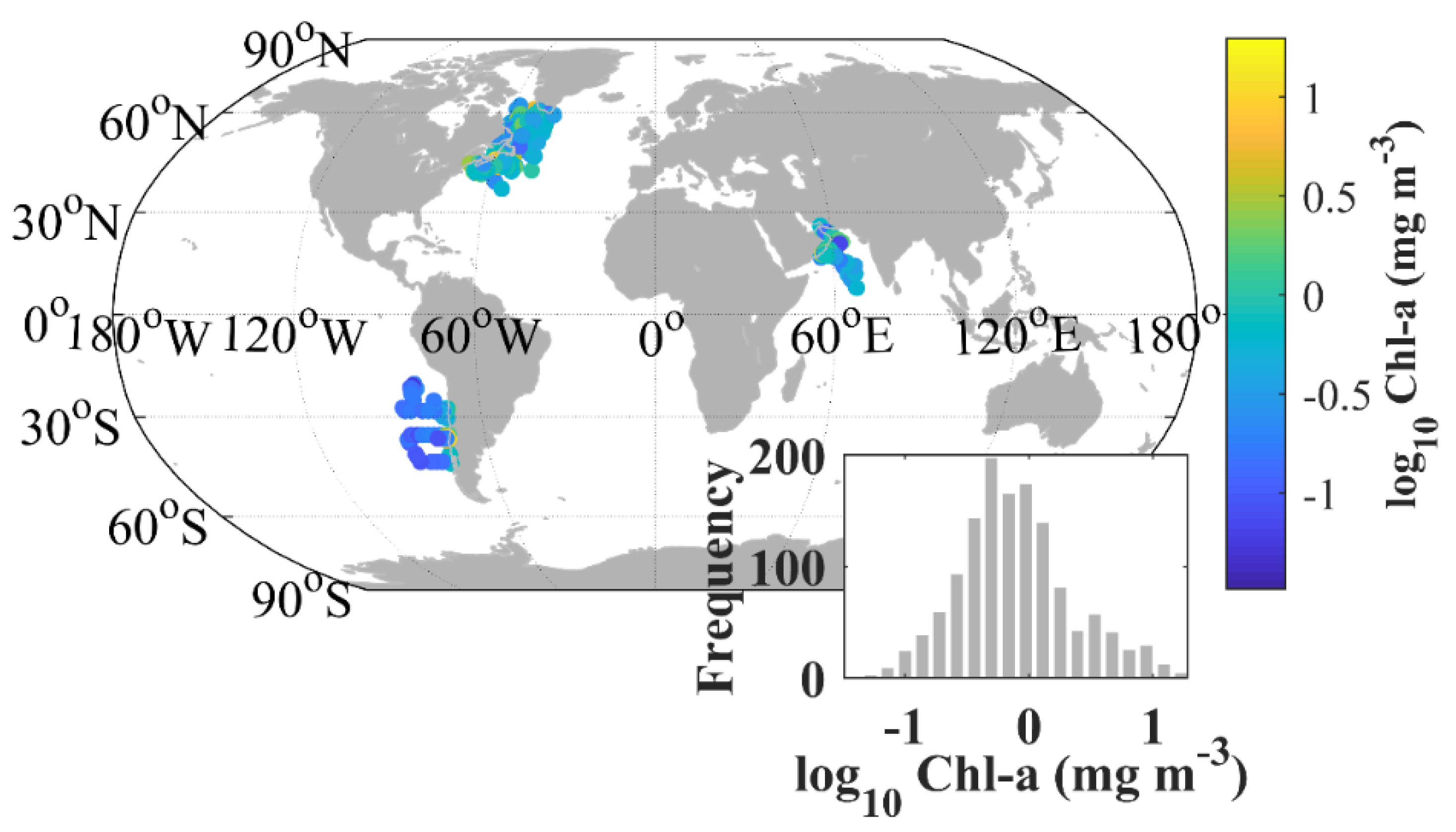
Figure 1.
Locations of sites where phytoplankton absorption spectra were measured together with concentrations of major pigments. Inset shows the distribution of all log-transformed chlorophyll-a (Chl-a) data.
Figure 1.
Locations of sites where phytoplankton absorption spectra were measured together with concentrations of major pigments. Inset shows the distribution of all log-transformed chlorophyll-a (Chl-a) data.
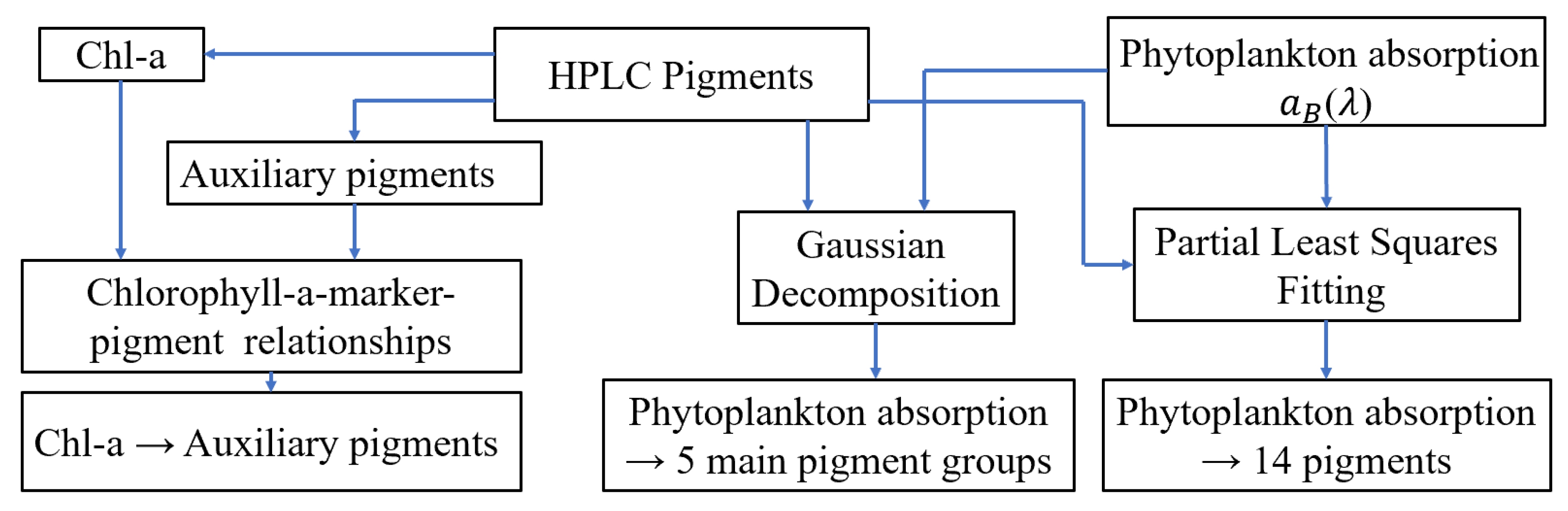
Figure 2.
Schematic overview of the data and processing steps used to estimate pigments from phytoplankton absorption and total chlorophyll-a (Chl-a) concentration.
Figure 2.
Schematic overview of the data and processing steps used to estimate pigments from phytoplankton absorption and total chlorophyll-a (Chl-a) concentration.
Figure 3.
Example of selection of a number of principal components calculated based on . The frequency of the minimum RMSE (gray column) and the frequency of the maximum r2 (green column) was calculated from 100 permutations for each pigment. The negative sign simply represents another type of parameter.
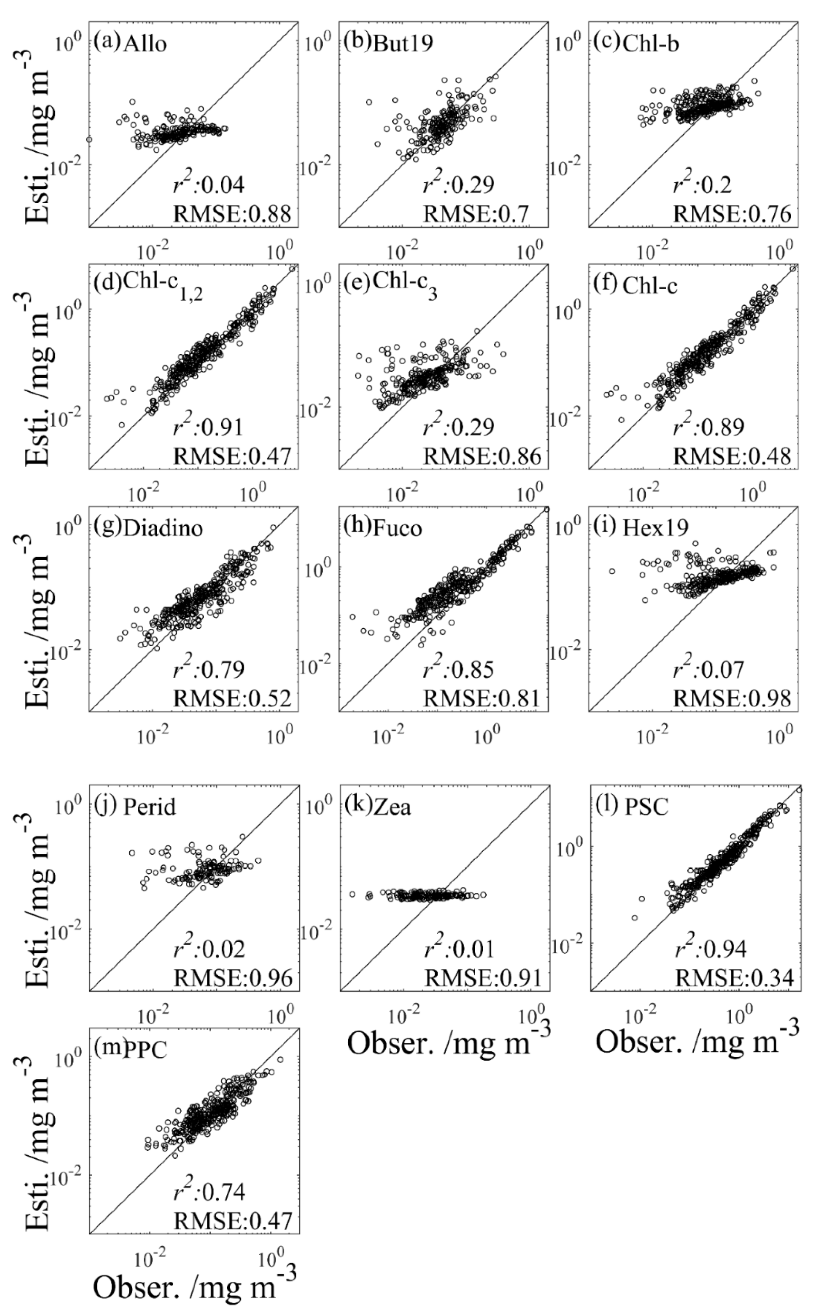
Figure 4.
Observed concentrations (Obser.) versus concentrations estimated from the Chl-a model (Esti.) of 13 phytoplankton pigments (a–m) using the testing set. The black line represents the 1:1 line.
Figure 4.
Observed concentrations (Obser.) versus concentrations estimated from the Chl-a model (Esti.) of 13 phytoplankton pigments (a–m) using the testing set. The black line represents the 1:1 line.
Figure 5.
Observed concentrations (Obser.) versus concentrations estimated from the Gaussian model (Esti.) of five main phytoplankton pigment groups (a–e) using the testing set. The black line represents the 1:1 line.
Figure 5.
Observed concentrations (Obser.) versus concentrations estimated from the Gaussian model (Esti.) of five main phytoplankton pigment groups (a–e) using the testing set. The black line represents the 1:1 line.
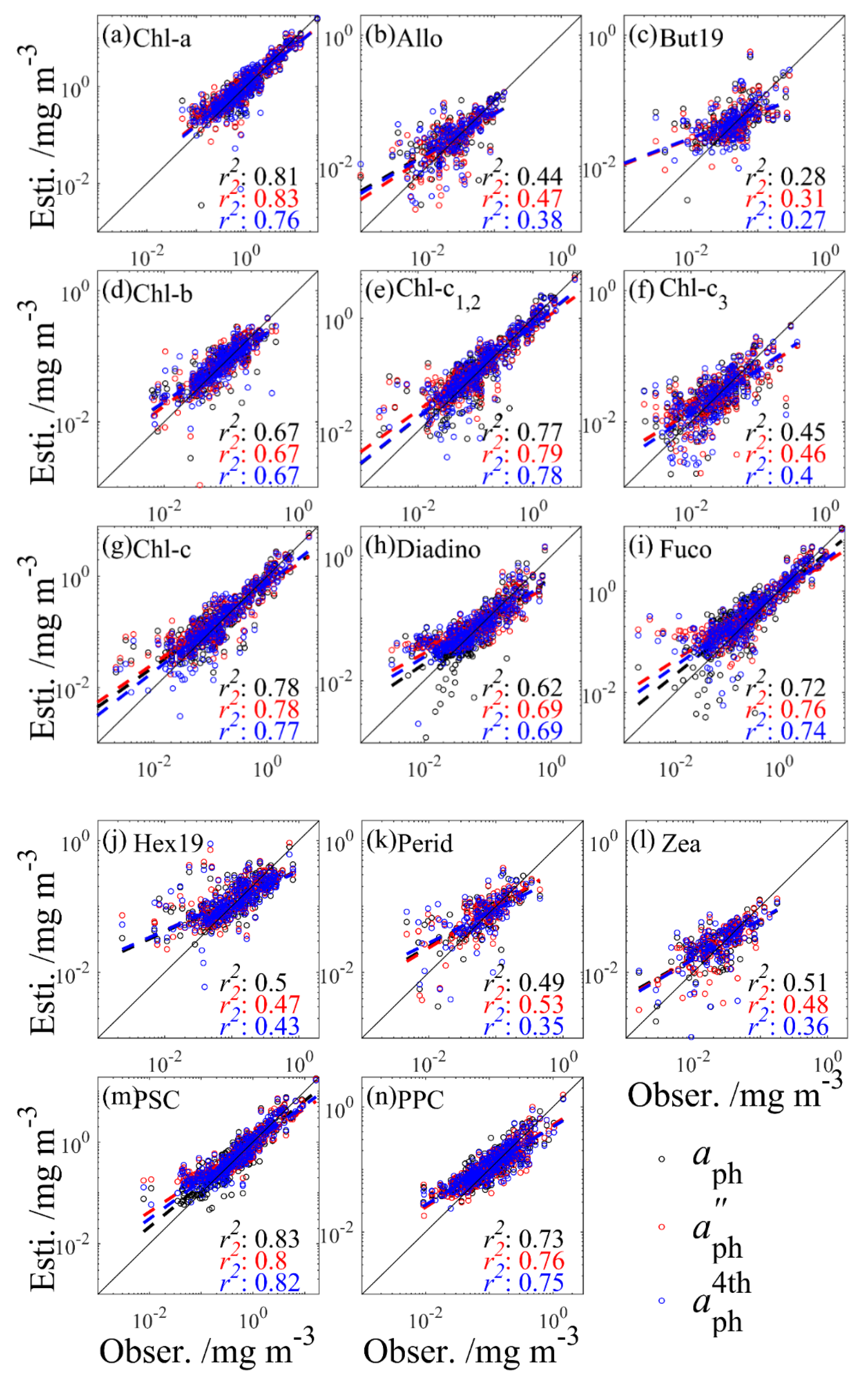
Figure 6.
Comparison of inversion performances derived by the PLS model of 14 phytoplankton pigments (a–n) using (black), (red), and (blue) as input. The best-fit line shows a first-order linear regression performed on the log-transformed data. The black line represents the 1:1 line. Results were obtained using the testing set together with the model tuned using the training set.
Figure 7.
Cross-validation (CV) statistics (r2CV, RMSECV, MAPDCV) between observed pigment concentrations and modeled pigment concentrations produced by the PLS model. Results for (black), (red), and (blue) are compared.
Figure 7.
Cross-validation (CV) statistics (r2CV, RMSECV, MAPDCV) between observed pigment concentrations and modeled pigment concentrations produced by the PLS model. Results for (black), (red), and (blue) are compared.
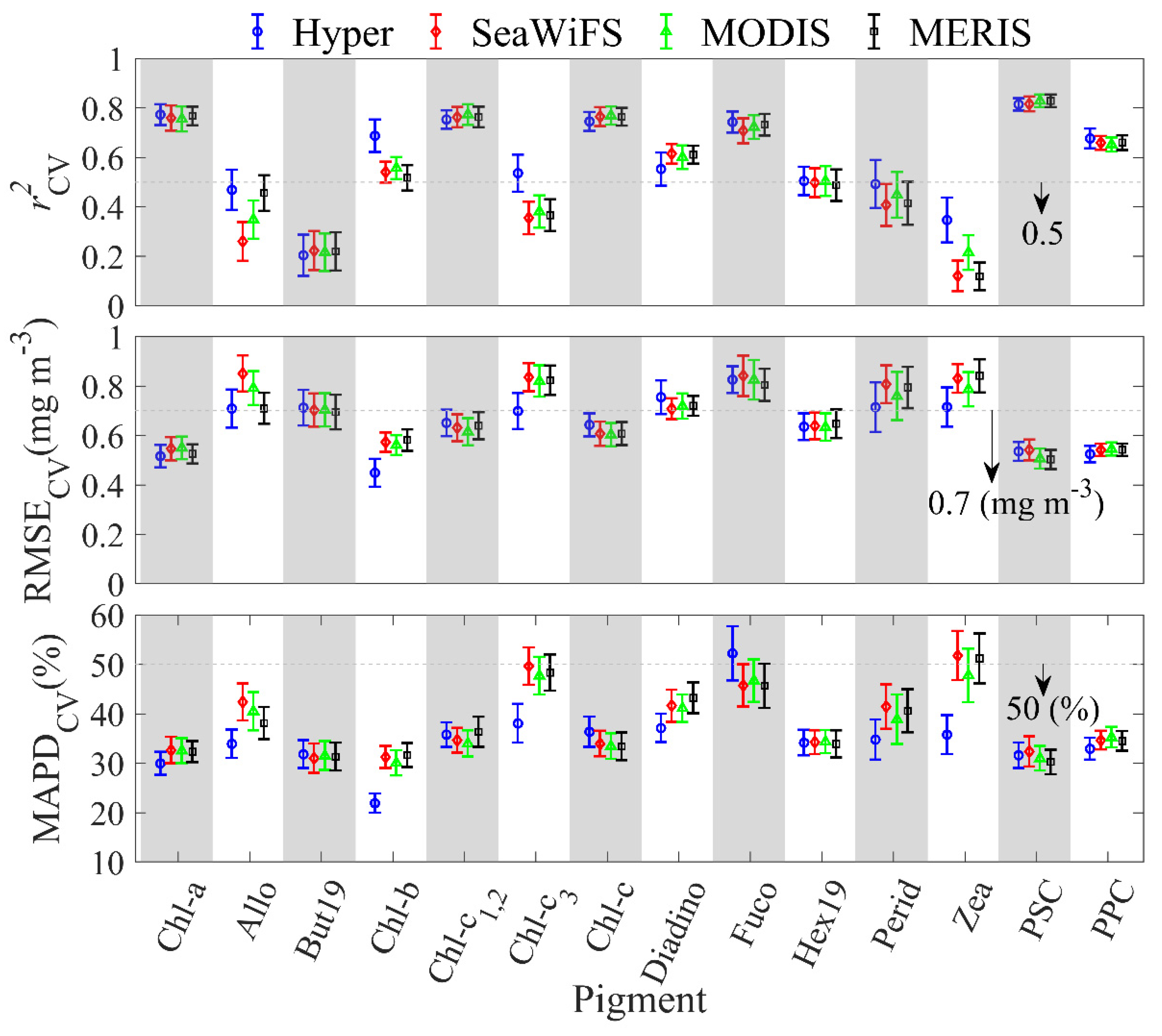
Figure 8.
Cross validation (CV) statistics (r2CV, RMSECV, and MAPDCV) between observed pigment concentrations and modeled pigment concentrations produced by the PLS model using hyperspectral , Multi_SeaWiFS, Multi_MODIS, and Multi_MERIS.
Figure 8.
Cross validation (CV) statistics (r2CV, RMSECV, and MAPDCV) between observed pigment concentrations and modeled pigment concentrations produced by the PLS model using hyperspectral , Multi_SeaWiFS, Multi_MODIS, and Multi_MERIS.
Figure 9.
Taylor diagrams illustrating the relative model performances of the Chl-a model, Gaussian model, and PLS model (based on , , , Multi_SeaWiFS, Multi_MODIS, and Multi_MERIS). The correlation coefficient, normalized standard deviation, and normalized RMSE are presented in the Taylor diagrams. The red dot labeled “A” represents perfect model performance. A model performs better if the retrievals are closer to the red dot A. All parameters were calculated based on log-transformed pigment concentration.
Table 1.
Name, abbreviation, and statistical distribution of pigments used in this study. Statistical distribution includes maximum (Max., mg m−3), minimum (Min., mg m−3), and standard deviation (std., mg m−3) of pigment concentrations. Pearson correlation coefficient (r) is estimated for linear regression between log-transformed concentrations of individual pigments and total chlorophyll-a. All statistics were calculated for values >0 mg m−3. Values of pigment concentrations below the limit of detection were considered zero.
| Name | Abbreviation | Min.–Max. (Std.) | r | N |
|---|
| chlorophyll-a | Chl-a 1 | 0.03–28.0 (2.41) | 1.00 | 1392 |
| alloxanthin | Allo | 0.001–0.24 (0.03) | 0.34 | 765 |
| 19′-butanoyloxy-fucoxanthin | But19 | 0.001–0.57 (0.05) | 0.49 | 762 |
| chlorophyll b | Chl-b 2 | 0.001–0.62 (0.07) | 0.47 | 1185 |
| chlorophyll-c1+ chlorophyll-c2 | Chl-c1,2 3 | 0.001–5.37 (0.48) | 0.95 | 1364 |
| chlorophyll-c3 | Chl-c3 | 0.001–0.39 (0.04) | 0.56 | 1036 |
| chlorophyll c | Chl-c 4 | 0.001–5.52 (0.50) | 0.94 | 1366 |
| diadinoxanthin | Diadino | 0.001–1.06 (0.11) | 0.88 | 1301 |
| fucoxanthin | Fuco | 0.001–16.6 (1.38) | 0.91 | 1325 |
| 19′-hexanoyloxy-fucoxanthin | Hex19 | 0.002–1.39 (0.13) | 0.43 | 1080 |
| peridinin | Perid | 0.003–0.53 (0.08) | 0.43 | 489 |
| zeaxanthin | Zea | 0.001–0.21 (0.03) | 0.04 | 626 |
| photosynthetic carotenoids | PSC 5 | 0.008–16.6 (1.35) | 0.97 | 1392 |
| photoprotective carotenoids | PPC 6 | 0.005–1.45 (0.13) | 0.84 | 1368 |
Table 2.
Central wavelengths of the Gaussian peak and the widths () of the Gaussian functions are assigned for different phytoplankton pigments (PE = phycoerythrin).
Table 2.
Central wavelengths of the Gaussian peak and the widths () of the Gaussian functions are assigned for different phytoplankton pigments (PE = phycoerythrin).
| | Chl-a | Chl-a | Chl-c | Chl-b | PPC | PSC | PE | Chl-c | Chl-a | Chl-c | Chl-b | Chl-a |
|---|
| Peak (nm) | 406 | 434 | 453 | 470 | 492 | 523 | 550 | 584 | 617 | 638 | 660 | 675 |
| (nm) | 17 | 13 | 12 | 14 | 17 | 15 | 15 | 17 | 14 | 11 | 11 | 10 |
Table 3.
Statistics for the Chl-a model including A and B in Equation (1), slope (S), intercept (I), and determination coefficient (r2) for the linear regression, root mean square error (RMSE, mg m−3), median absolute percent difference (MAPD, %), and bias (Bias, mg m−3).
Table 3.
Statistics for the Chl-a model including A and B in Equation (1), slope (S), intercept (I), and determination coefficient (r2) for the linear regression, root mean square error (RMSE, mg m−3), median absolute percent difference (MAPD, %), and bias (Bias, mg m−3).
| Pigment | For Training Set | For Testing Set |
|---|
| A | B | r2 | S | I | r2 | RMSE | MAPD | Bias |
|---|
| Allo | 0.04 | 0.33 | 0.14 | 0.07 | −3.14 | 0.04 | 0.88 | 54.0 | 0.34 |
| But19 | 0.06 | 0.61 | 0.22 | 0.40 | −1.80 | 0.29 | 0.70 | 29.1 | 0.14 |
| Chl-b | 0.09 | 0.26 | 0.23 | 0.16 | −1.97 | 0.20 | 0.76 | 40.82 | 0.27 |
| Chl-c1,2 | 0.16 | 1.07 | 0.91 | 0.82 | −0.22 | 0.91 | 0.47 | 24.9 | 0.17 |
| Chl-c3 | 0.03 | 0.49 | 0.32 | 0.30 | −2.30 | 0.29 | 0.86 | 44.6 | 0.34 |
| Chl-c | 0.18 | 1.04 | 0.89 | 0.80 | −0.26 | 0.89 | 0.48 | 27.7 | 0.14 |
| Diadino | 0.07 | 0.77 | 0.76 | 0.69 | −0.71 | 0.79 | 0.52 | 39.3 | 0.17 |
| Fuco | 0.41 | 1.09 | 0.82 | 0.69 | 0.04 | 0.85 | 0.81 | 62.2 | 0.48 |
| Hex19 | 0.17 | 0.33 | 0.25 | 0.10 | −1.68 | 0.07 | 0.98 | 50.0 | 0.36 |
| Perid | 0.09 | 0.49 | 0.27 | 0.07 | −2.23 | 0.02 | 0.96 | 46.5 | 0.36 |
| Zea | 0.04 | 0.07 | 0.00 | 0.00 | −3.37 | 0.01 | 0.91 | 60.8 | 0.39 |
| PSC | 0.57 | 0.96 | 0.93 | 0.86 | −0.01 | 0.94 | 0.34 | 17.6 | 0.11 |
| PPC | 0.12 | 0.59 | 0.68 | 0.64 | −0.70 | 0.74 | 0.47 | 31.6 | 0.12 |
Table 4.
Statistics for the Gaussian model including A2 and B2 for Equation (3), slope (S), intercept (I), and determination coefficient (r2) for the linear regression, root mean square error (RMSE, mg m−3), median absolute percent difference (MAPD, %), and bias (Bias, mg m−3).
Table 4.
Statistics for the Gaussian model including A2 and B2 for Equation (3), slope (S), intercept (I), and determination coefficient (r2) for the linear regression, root mean square error (RMSE, mg m−3), median absolute percent difference (MAPD, %), and bias (Bias, mg m−3).
| Pigment | For Training Set | For Testing Set |
|---|
| A2 | B2 | r2 | S | I | r2 | RMSE | MAPD | Bias |
|---|
| Chl-a_406 | 32.8 | 1.05 | 0.70 | 0.77 | 0.18 | 0.82 | 0.53 | 39.5 | 0.22 |
| Chl-a_434 | 59.5 | 1.21 | 0.71 | 0.79 | 0.11 | 0.76 | 0.57 | 41.7 | 0.15 |
| Chl-a_617 | 229 | 1.01 | 0.73 | 0.87 | 0.11 | 0.85 | 0.45 | 28.1 | 0.13 |
| Chl-a_675 | 67.0 | 1.08 | 0.84 | 0.89 | 0.10 | 0.86 | 0.44 | 29.4 | 0.12 |
| Chl-b_470 | 0.6 | 0.51 | 0.30 | 0.29 | −1.66 | 0.35 | 0.68 | 39.9 | 0.23 |
| Chl-b_660 | 0.4 | 0.28 | 0.28 | 0.17 | −1.96 | 0.20 | 0.75 | 43.5 | 0.25 |
| Chl-c_584 | 56.9 | 1.10 | 0.67 | 0.71 | −0.29 | 0.75 | 0.73 | 45.4 | 0.28 |
| Chl-c_638 | 56.3 | 1.13 | 0.74 | 0.73 | −0.29 | 0.74 | 0.74 | 44.1 | 0.25 |
| PSC_523 | 80.4 | 1.10 | 0.66 | 0.79 | 0.05 | 0.84 | 0.55 | 34.1 | 0.23 |
| PPC_492 | 3.1 | 0.89 | 0.66 | 0.67 | −0.66 | 0.70 | 0.49 | 31.2 | 0.10 |
Table 5.
Statistics for the PLS model including the explained variance for independent (X, %) and dependent (Y, %) variables corresponding to the relative PCN (see
Table 6), slope (
S), intercept (
I), determination coefficient (
r2) for the linear regression, root mean square error (RMSE, mg m
−3), median absolute percent difference (MAPD, %), and bias (Bias, mg m
−3).
| Pigment | For Training Set | For Testing Set |
|---|
| X | Y | r2 | S | I | r2 | RMSE | MAPD | Bias |
|---|
| Chl-a | 99.99 | 91.51 | 0.77 | 0.82 | 0.05 | 0.81 | 0.50 | 27.0 | 0.08 |
| Allo | 99.99 | 69.40 | 0.48 | 0.59 | −1.41 | 0.44 | 0.66 | 26.0 | 0.12 |
| But19 | 99.99 | 48.54 | 0.22 | 0.38 | −1.86 | 0.28 | 0.70 | 25.7 | 0.13 |
| Chl-b | 99.99 | 69.68 | 0.71 | 0.69 | −0.76 | 0.67 | 0.45 | 23.6 | 0.08 |
| Chl-c1,2 | 99.83 | 89.87 | 0.76 | 0.82 | −0.29 | 0.77 | 0.68 | 34.1 | 0.10 |
| Chl-c3 | 99.99 | 72.67 | 0.56 | 0.63 | −1.37 | 0.45 | 0.74 | 43.1 | 0.05 |
| Chl-c | 99.91 | 90.19 | 0.75 | 0.73 | −0.38 | 0.78 | 0.65 | 33.8 | 0.15 |
| Diadino | 99.91 | 73.65 | 0.52 | 0.69 | −0.81 | 0.62 | 0.66 | 34.1 | 0.08 |
| Fuco | 99.84 | 81.17 | 0.75 | 0.82 | −0.02 | 0.72 | 0.86 | 48.7 | 0.23 |
| Hex19 | 99.84 | 52.84 | 0.50 | 0.47 | −1.03 | 0.50 | 0.69 | 33.5 | 0.17 |
| Perid | 99.99 | 62.41 | 0.52 | 0.59 | −0.97 | 0.49 | 0.63 | 27.8 | 0.14 |
| Zea | 99.99 | 58.85 | 0.38 | 0.57 | −1.47 | 0.51 | 0.60 | 38.0 | 0.15 |
| PSC | 99.84 | 80.92 | 0.82 | 0.83 | −0.04 | 0.83 | 0.51 | 28.6 | 0.11 |
| PPC | 99.88 | 68.73 | 0.77 | 0.65 | −0.70 | 0.73 | 0.48 | 32.5 | 0.11 |
Table 6.
The PCN for each pigment when different types of spectra are used, which includes , , , Multi_SeaWiFS, Multi_MODIS, and Multi_MERIS.
Table 6.
The PCN for each pigment when different types of spectra are used, which includes , , , Multi_SeaWiFS, Multi_MODIS, and Multi_MERIS.
| Pigment | Hyperspectral | Multispectral |
|---|
| | | Multi_SeaWiFS | Multi_MODIS | Multi_MERIS |
|---|
| Chl-a | 11 | 4 | 3 | 3 | 2 | 5 |
| Allo | 12 | 10 | 11 | 5 | 6 | 7 |
| But19 | 9 | 8 | 8 | 5 | 5 | 5 |
| Chl-b | 9 | 8 | 15 | 6 | 7 | 7 |
| Chl-c1,2 | 3 | 3 | 4 | 5 | 5 | 3 |
| Chl-c3 | 13 | 9 | 15 | 5 | 6 | 5 |
| Chl-c | 4 | 3 | 3 | 5 | 5 | 5 |
| Diadino | 5 | 2 | 3 | 4 | 7 | 4 |
| Fuco | 3 | 2 | 3 | 4 | 4 | 4 |
| Hex19 | 3 | 3 | 3 | 3 | 3 | 6 |
| Perid | 12 | 11 | 15 | 3 | 7 | 8 |
| Zea | 15 | 15 | 7 | 4 | 7 | 8 |
| PSC | 3 | 2 | 3 | 2 | 4 | 4 |
| PPC | 4 | 4 | 3 | 6 | 3 | 6 |
Table 7.
Mean statistics of the CV of 500 permutations based on S_train and S_test for the three model types, i.e., the Chl-a model, Gaussian model, and PLS model based on hyper (λ). For the Gaussian model, the optimum performance for each pigment was chosen for presentation here.
Table 7.
Mean statistics of the CV of 500 permutations based on S_train and S_test for the three model types, i.e., the Chl-a model, Gaussian model, and PLS model based on hyper (λ). For the Gaussian model, the optimum performance for each pigment was chosen for presentation here.
| Pigment | r2CV | RMSECV | MAPDCV | BiasCV | rCV |
|---|
| Chl-a model |
| Allo | 0.16 | 0.94 | 55.20 | 0.37 | 0.39 |
| But19 | 0.22 | 0.70 | 31.70 | 0.13 | 0.47 |
| Chl-b | 0.23 | 0.75 | 39.97 | 0.24 | 0.47 |
| Chl-c1,2 | 0.91 | 0.42 | 24.64 | 0.15 | 0.95 |
| Chl-c3 | 0.33 | 0.89 | 50.67 | 0.35 | 0.57 |
| Chl-c | 0.89 | 0.42 | 27.37 | 0.11 | 0.95 |
| Diadino | 0.76 | 0.61 | 39.26 | 0.26 | 0.87 |
| Fuco | 0.82 | 0.84 | 57.34 | 0.49 | 0.91 |
| Hex19 | 0.25 | 0.83 | 47.67 | 0.32 | 0.50 |
| Perid | 0.27 | 0.95 | 46.35 | 0.36 | 0.52 |
| Zea | 0.01 | 0.89 | 53.44 | 0.30 | 0.06 |
| PSC | 0.93 | 0.34 | 19.71 | 0.13 | 0.97 |
| PPC | 0.69 | 0.53 | 32.18 | 0.17 | 0.83 |
| Gaussian model based on |
| Chl-a_675 | 0.83 | 0.47 | 30.64 | 0.15 | 0.91 |
| Chl-b_470 | 0.41 | 0.66 | 35.45 | 0.21 | 0.64 |
| Chl-c_584 | 0.71 | 0.71 | 42.97 | 0.25 | 0.84 |
| PSC_523 | 0.81 | 0.57 | 37.18 | 0.25 | 0.90 |
| PPC_492 | 0.66 | 0.53 | 34.25 | 0.14 | 0.81 |
| PLS model based on |
| Chl-a | 0.77 | 0.52 | 29.95 | 0.11 | 0.88 |
| Allo | 0.47 | 0.71 | 33.91 | 0.12 | 0.68 |
| But19 | 0.20 | 0.71 | 31.81 | 0.14 | 0.44 |
| Chl-b | 0.69 | 0.45 | 21.91 | 0.08 | 0.83 |
| Chl-c1,2 | 0.75 | 0.65 | 35.78 | 0.16 | 0.87 |
| Chl-c3 | 0.54 | 0.70 | 38.05 | 0.14 | 0.73 |
| Chl-c | 0.75 | 0.64 | 36.37 | 0.19 | 0.86 |
| Diadino | 0.55 | 0.76 | 37.10 | 0.20 | 0.74 |
| Fuco | 0.74 | 0.83 | 52.22 | 0.33 | 0.86 |
| Hex19 | 0.51 | 0.64 | 34.15 | 0.15 | 0.71 |
| Perid | 0.49 | 0.72 | 34.77 | 0.14 | 0.70 |
| Zea | 0.35 | 0.72 | 35.78 | 0.15 | 0.58 |
| PSC | 0.82 | 0.54 | 31.61 | 0.16 | 0.90 |
| PPC | 0.68 | 0.53 | 32.91 | 0.15 | 0.82 |


 ,
, 


