Flood Discharge Prediction Based on Remote-Sensed Spatiotemporal Features Fusion and Graph Attention

Abstract

Floods have brought a great threat to the life and property of human beings. Under the premise of strengthening flood control engineering measures and following the strategic thinking of sustainable development, many achievements have been made in flood forecasting recently. However, due to the complexity of the traditional lumped model and distributed model, the hydrologic parameter calibration process is full of difficulties, leading to a long development cycle of a reasonable hydrologic prediction model. Even for modern data-driven models, the spatial distribution characteristics of the rainfall data are also not fully mined. Based on this situation, this paper abstracts the rainfall data into the graph structure data, uses remote sensing images to extract the elevation information, introduces the graph attention mechanism to extract the spatial characteristics of rainfall, and employs long-term and short-term memory (LSTM) network to fuse the spatial and temporal characteristics for flood prediction. Through well-designed experiments, the forecasting effect of flood peak value and flood arrival time is verified. Furthermore, compared with the LSTM model and BIGRU model without spatial feature extraction, the advantages of spatiotemporal feature fusion are highlighted. The specific performance is that the RMSE (the root means square error) and $R^2$ (coefficient of determination) of the GA-RNN model have been significantly improved. Finally, we conduct experiments on the observed ten rainfall events in the history of the target watershed. According to the hydrological prediction specifications, the model can be evaluated as a Class B flood forecasting model.

1. Introduction

Floods are one of the most common natural disasters in the world. Compared with other natural disasters, the loss of people’s material property and the increase of social instability caused by floods have made them the most prominent in all kinds of disasters for a long time [1,2]. Each year, floods kill thousands to tens of thousands of people, affect the lives of hundreds of millions, and cause tens of billions of dollars in damage [3,4,5]. If there are no timely preventive measures for floods, it will lead to greater damage, such as easily causing traffic jams, plague, and other problems. Therefore, determining how to effectively reduce or avoid the disasters caused by floods is very necessary.

In past flood forecasting, the models used were mainly physically based [6]. For example, the literature [7] pointed out the correlation between rainfall and runoff, and the water level was predicted in 72 test cases in eight different cities. The effect is very satisfactory, which also points out to us that it is desirable and necessary to calculate the rainfall–runoff conversion from direct rainfall data. The disadvantage is that the the cost of calculation is relatively high. The literature [8] uses three methods (fully dynamic, diffusive, and kinematic waves) to mathematically describe the surface flow. The full dynamic model can make good predictions of flow and water level, but the pros and cons of the model are very limited by the grid size. The literature [9] used a shallow water surface flow model to test a certain area in the UK, and the results were good, but the calculation of the model was very complicated. Literature [10] considers the interaction between water flow and man-made structures (bridges, weirs, buildings, etc.) based on flow dynamics and demonstrates a case. The article points out that there are many influencing factors in flood dynamics and suggests inserting different types of hydrological data for learning in two-dimensional hydraulics, but in fact, we know that there are too many influencing factors of floods, and it is difficult for us to fully simulate them. Although physically based models show a strong ability to predict various flood scenarios, they often require various types of hydrological and geomorphological monitoring data sets, and the setup and operation of models are very time-consuming, which hinders short-term prediction [11]. In addition, as mentioned in reference [12], the development of physically based models usually requires in-depth knowledge and expertise on hydrological parameters, which is very challenging and not conducive to the promotion of hydrological models.

With the acceleration of the digital process, a lot of historical hydrological data has been preserved. In addition, with the improvement of computer computing power [13], large-scale data-driven models that used to take several months can now converge and obtain optimized results in just weeks or even hours, making data-driven flood forecasting models appear in large numbers. Examples are ANNs (Artificial Neural Networks) [14], neuro-fuzzy [15], adaptive neuro-fuzzy inference systems [16], support vector machines (SVM) [17], etc. However, common data-driven models treat flood forecasting tasks as sequence-to-sequence conversion work, treat the input rainfall data only as a time series, and use the RNN (Recurrent Neural Network) and its variant structures to analyze time-series information. For example, Xu Yuanhao [18] and his colleagues simulated and predicted the flood and waterlogging process in the middle reaches of the Yellow River based on the LSTM (Long Short-Term Memory) network and extracted the temporal characteristics by inputting the rainfall data of 14 areas in the upper reaches of the Yellow River into the LSTM network at one time. Because the spatial distribution of rainfall in different areas was not considered, the prediction effect of the whole model decreased significantly when the prediction period was more than 6 h. Francis Yongwa Dtissibe [19] and others used the multi-layer perceptron in order to design a flood forecasting model and only used discharge as input–output variables. This model also regards flood forecasting tasks as sequence-to-sequence conversion work. Although, the model can accurately predict future discharge on the hydrological station at the Gardon d’Anduze, a river found in the Gard Division (France), Anduze Township. However, the forecast period of the model is only one hour, and other factors (rainfall, temperature, etc.) are not considered. Experiments of the model are only conducted on one station. The model undoubtedly has certain defects in multiple hydrological stations and multiple rivers. Liang Xiaoxu [20] and others improved the BIGRU (Bidirectional Gate Recurrent Unit) model, introduced the attention mechanism, calculated the weighted summation output by using the attention weight, and realized the high-precision forecast of Xixianhe River Basin in the 36 h forecast period. Because the model is only a deep mining network of time-series information, it does not take into account the spatial distribution information of rainfall and is insensitive to the rainstorm in some small areas.

For many types of data, there are obvious spatial distributions, such as the traffic flow distribution in the traffic flow prediction task [21,22], the spatial distribution of pixels in the computer vision task [23,24], and the rainfall data distribution in a certain area. In the task of vehicle flow prediction, there are many temporal and spatial feature fusion schemes. Based on the principle of support vector machine, Li qiaoru [25] and others designed an adaptive spatiotemporal feature fusion model to dynamically update the weights of spatiotemporal feature fusion. In computer vision, the classical convolutional neural network obtains deep-seated features by mining the spatial distribution of image pixels. Zhao Zhihong [26] and others used the convolution neural network LeNet 5 to recognize the license plate, and the accuracy was 98%. In the field of flood forecasting, Yukai Ding [27] and others propose an interpretable Spatio-Temporal Attention Long Short Term Memory model (STA-LSTM) based on LSTM and attention mechanism. The model can realize the dynamic adjustment of the weight through the time attention mechanism and the space attention mechanism module, which better simulates the real rainfall convergence process. However, it did not give a detailed description of the specific convergence relationship of rainfall data and did not use spatial information between rainfall stations to analyze the convergence relationship of rainfall data. Amir Mosavi [28] and others applied the Normalized Difference Vegetation Index (NDVI) to runoff prediction and developed a simple spatiotemporal model based on the Generalized Structure of Group Method of Data Handling (GSGMDH). The inputs of the model are rainfall, runoff, and NDVI data. The NDVI is an important factor reflecting the change of runoff. NDVI index values are between +1 and −1. The NDVI for water, cloud, and snow cover phenomena are negative, while this parameter for bare soil and sand is positive and close to zero. Besides, healthy and lush vegetation has positive NDVI values (0.2–0.8). The NDVI value can truly reflect the geographic information of the area [29]. Although the model has achieved good prediction results, the acquisition and processing of NDVI data are very complicated, so the model is not universal. Furthermore, the increase in runoff predicted by the model in autumn and winter may be related to the similarity of the NDVI values of water, clouds, and snow. The extraction of spatial information is not enough.

Effective mining of spatial information is essential to improve the accuracy of prediction. To fully excavate the spatial distribution information of rainfall and improve the overall predictive ability of the model, this paper uses remote sensing images to extract digital elevation information of the target basin. Using the digital elevation information of the target basin, the topography of the target basin can be truly known, so that the convergence relationship between rainfall stations can be expressed more realistically. The rainfall station is abstracted as a node, and the convergence relationship between the rainfall stations is determined according to the digital elevation information of the target basin and the geographic location information of the rainfall station. Based on this, a spatiotemporal feature fusion model GA-RNN (Graph Attention Recurrent Neural Network) method based on graph attention mechanism [30] is proposed. The contributions are as follows:

(1)

Use the digital elevation information extracted from remote sensing images to convert rainfall data into graph data and design a GA-RNN model based on graph attention mechanism to extract the spatial characteristics of rainfall.

(2)

Compared with the model without spatial feature extraction, it proves the performance improvement brought by spatiotemporal feature fusion.

(3)

Ten flood events were selected to evaluate the GA-RNN model.

This article is organized as follows. The first part introduces the research significance and current situation. The second part introduces the research data processing scheme and the calculation process of GAT (Graph Attention Mechanism). The third part introduces in detail the structural parameters and training effects of GA-RNN based on the graph attention mechanism model and gives relevant statistics and comparative experiments. The fourth part is the discussion part, explaining and analyzing the experimental data of the fourth part. The fifth part summarizes the full-text research.

2. Data Processing and Model Introduction

2.1. Data Profile and Preprocessing

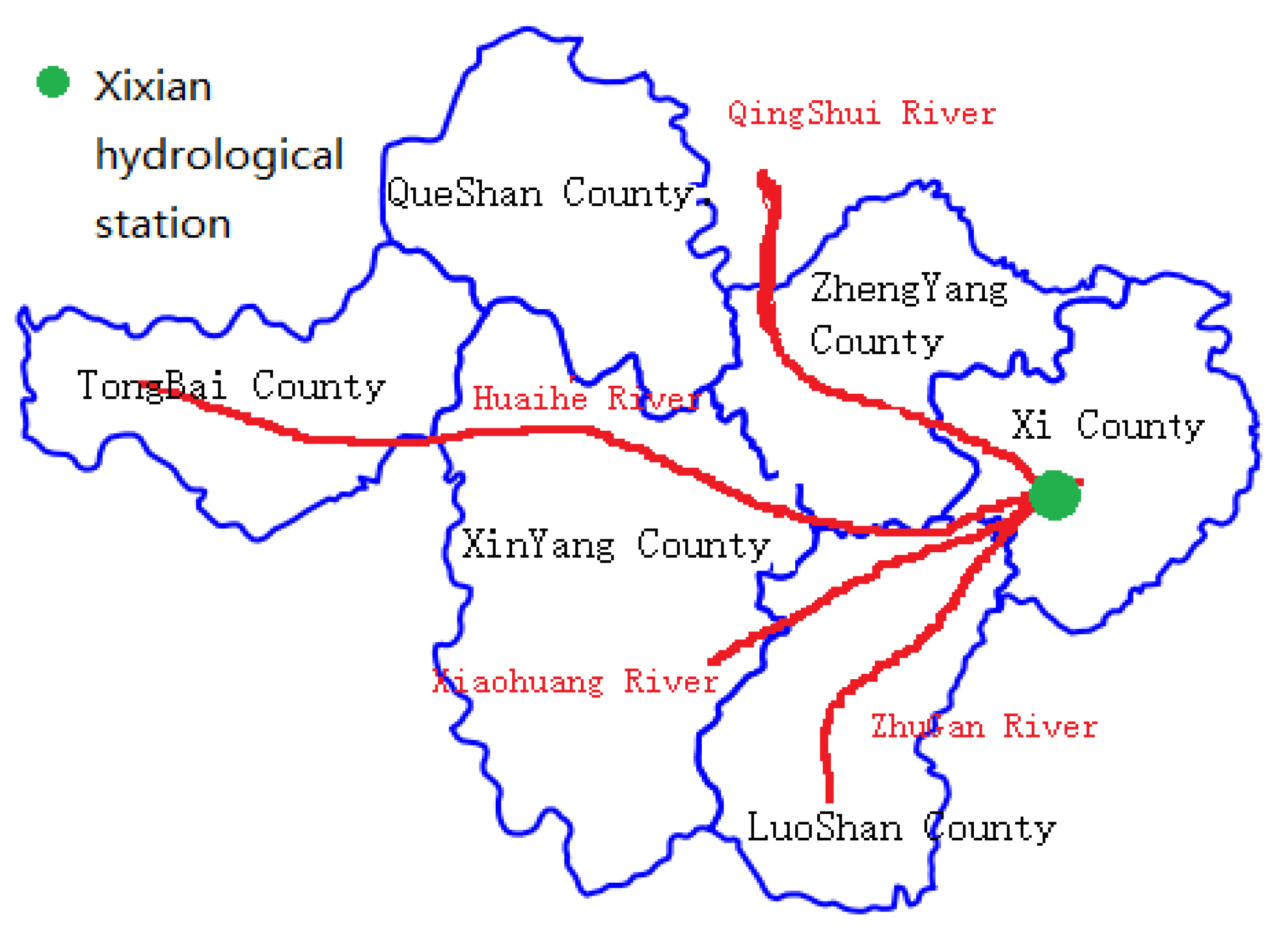
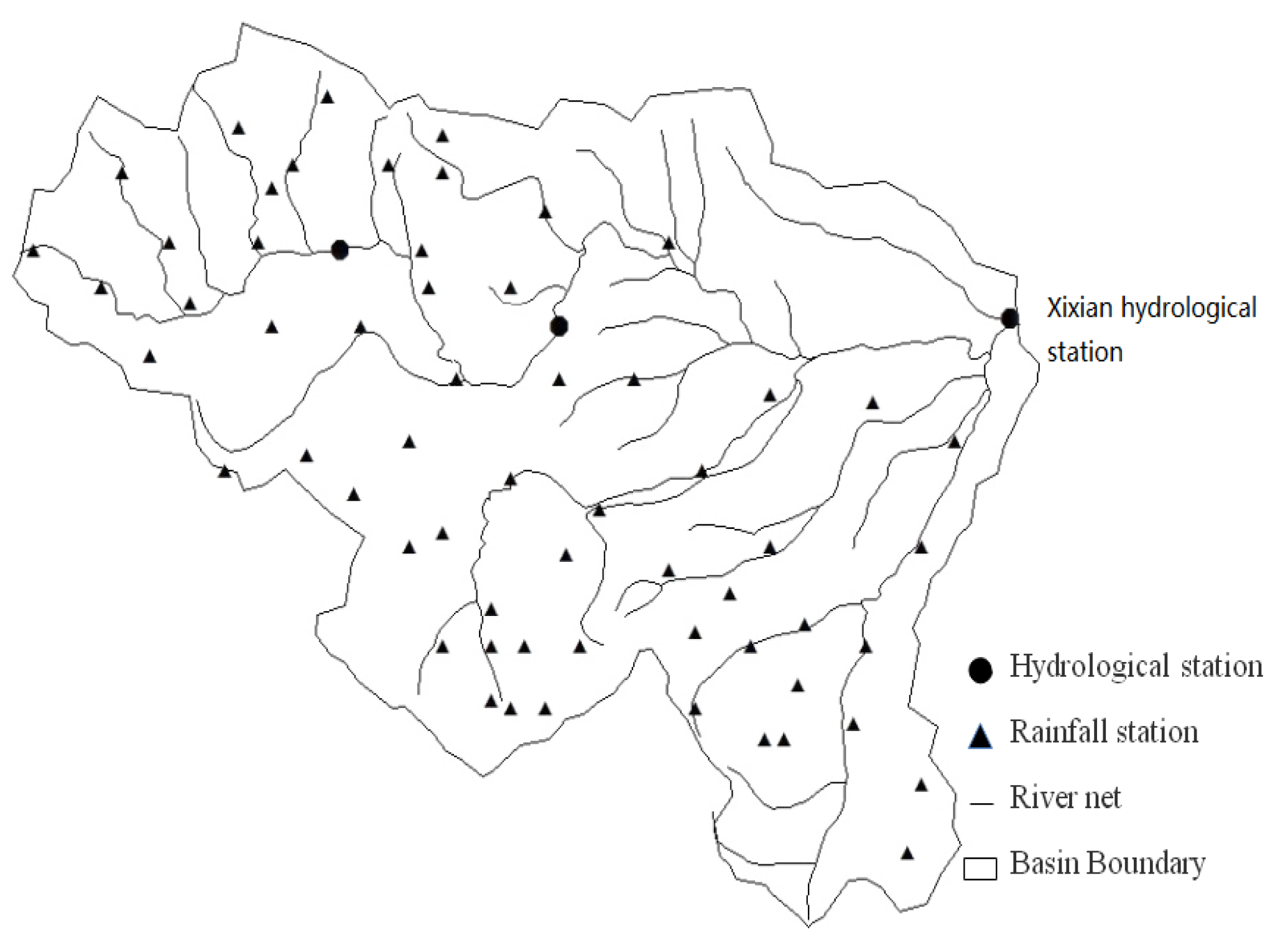
The area studied in this paper is the Xi county in Henan Province, which is located in the Huaihe River Basin, with low mountains and hills as its main topographic features. Huaihe River, Qingshui River, Xiaohuanghe River, Zhugan River, and other rivers flow together in Xixian hydrological station. From June to July every year, influenced by the monsoon, the river water level and flow change in a large range. Figure 1 shows the geographical location of the Xixian hydrological station and the main rivers flowing through the basin. Figure 2 shows the distribution of the Xixian hydrological station and rainfall stations in the basin. The purpose of this study is to analyze the rainfall data of the target basin and predict the river flow of Xixian hydrological station downstream of the target basin.

Because of its terrain characteristics, the rainfall in the whole region quickly converges to Xixian hydrological station through the main rivers, which makes Xixian hydrological station have the characteristics of a large amount of water, the rapid rise of water level, and high flood peak value in flood season, which brings great pressure to flood control. Because of this, many studies try to apply the hydrological forecasting model to flood disaster early warning in Xi county to reduce losses. The school of hydrology and meteorology of Nanjing University of information engineering has applied the Xin’anjiang model and other traditional models in Xi county and adopted the multi-model integrated forecasting method, which has achieved good discharge forecasting results. Qian Mingkai and others of the Hydrological Bureau of Huaihe Water Resources Commission established a flood probability prediction framework based on Bayesian statistical theory, which also has a high application value for flood probability prediction in Xi county. Based on the same research goal, this paper uses the rainfall and flow data of the target basin from 2010 to 2018 to establish a flood flow prediction model based on the fusion of spatiotemporal characteristics of machine learning and achieves satisfactory results in the prediction of flood peak and flood arrival time.

2.1.1. Water Flow Data Preprocessing

The structure and identifier document of the real-time rain water regime database table is ST_ RIVER_ R. It is used to store the river information measured by the hydrological station and record the river water level and flow information at some time points in detail. The record format of the original data is shown in

Table 1. Flow data table fields of the Xixian hydrological station.

Field Name	Data Type	Unit	Notes
TM	Date	/	Recording time
Q	Floating point number	m${}^3$/s	water flow
Z	Floating point number	m	water level

.

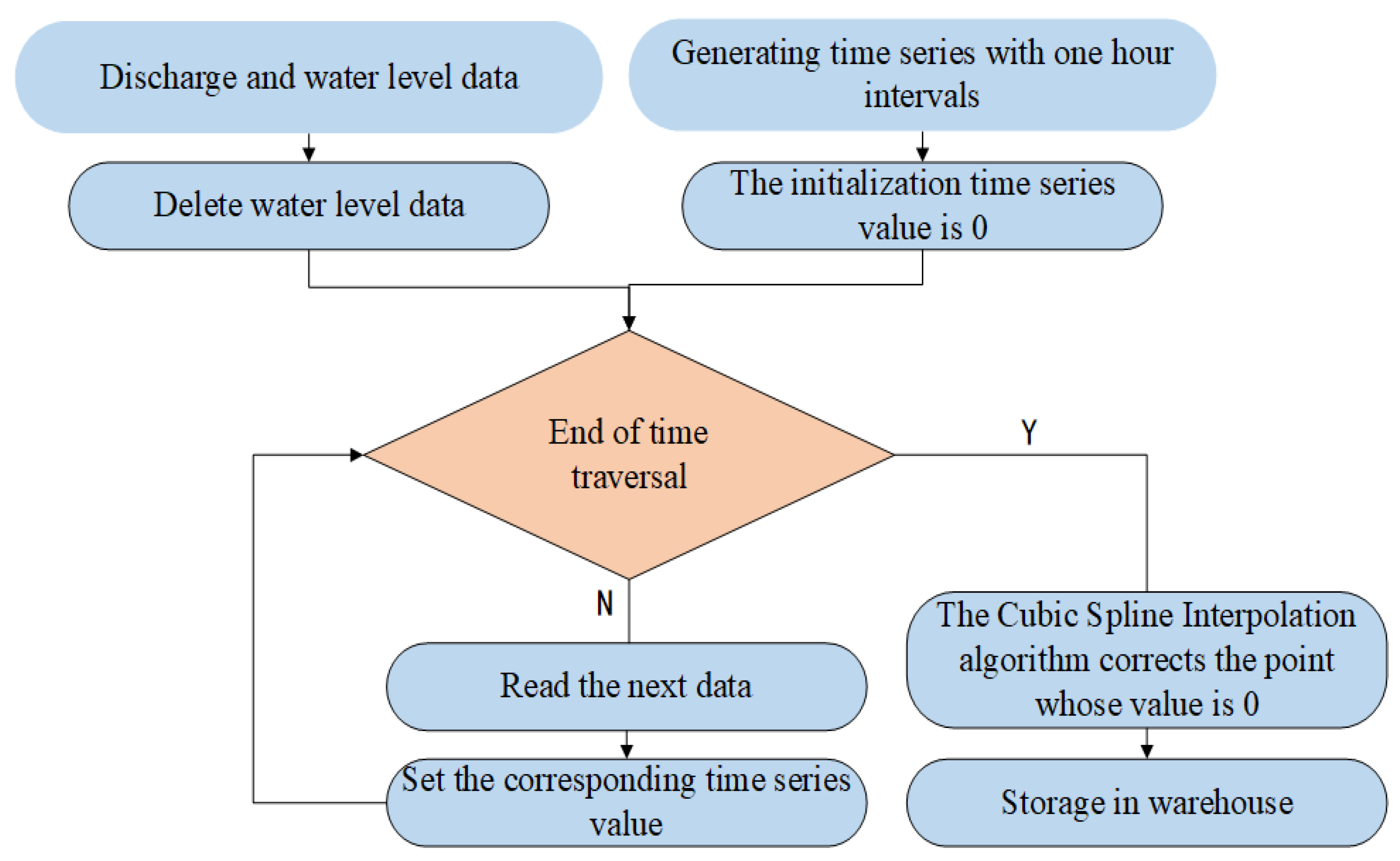
The time interval for recording Q and Z in the original data is one hour. There may be some missing values in the data due to equipment failure or other reasons. For missing values, we use cubic spline interpolation to fill in. As shown in Figure 3, we preprocessed the original flood flow data.

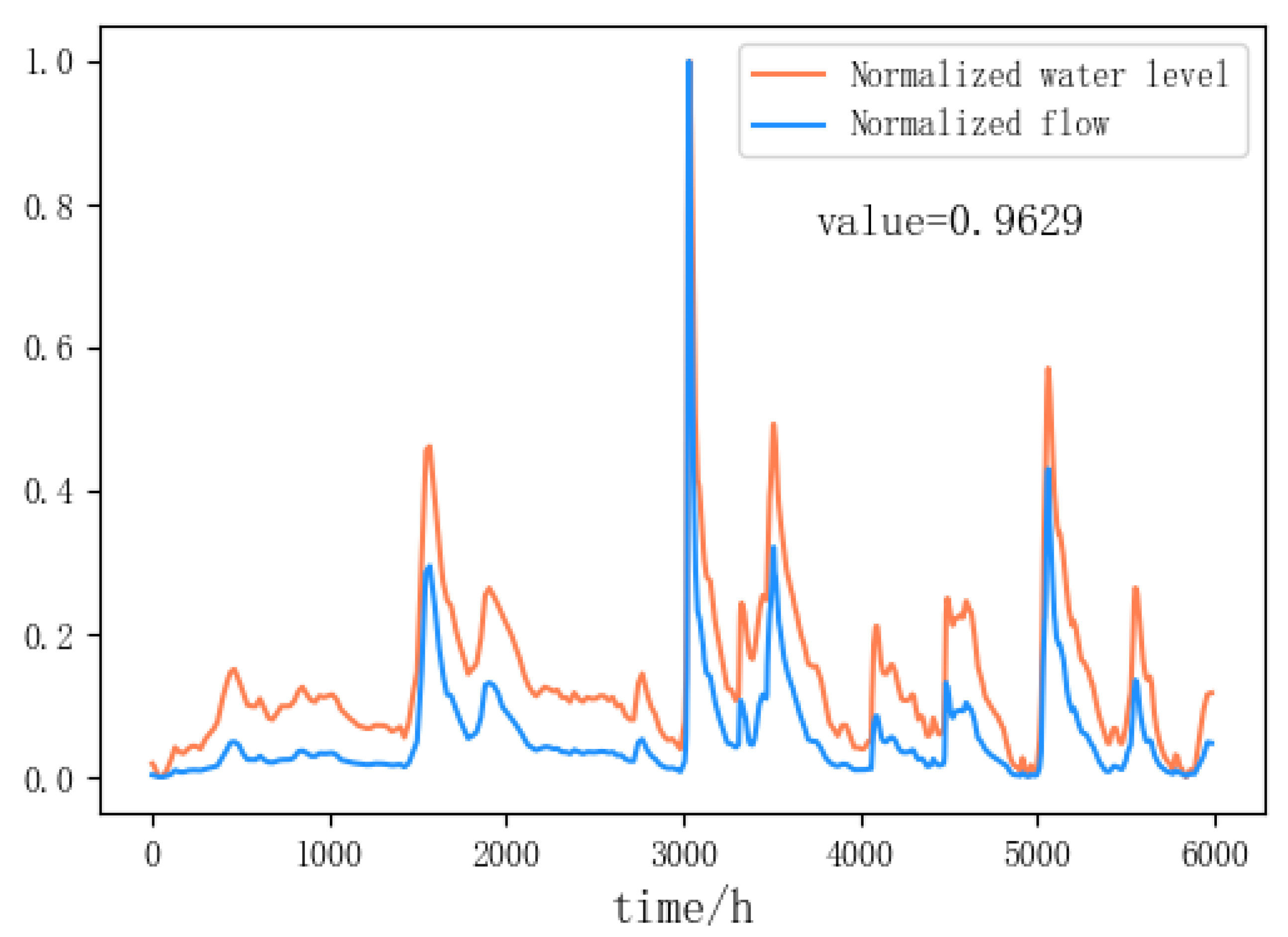
In the process of processing, considering the high correlation between water level data and discharge data, in 2018, for example, the curve after numerical scaling is shown in Figure 4. From the curve trend, the two maintain a high degree of consistency. Use Formula (1) to calculate the Pearson correlation coefficient of the two, and the result is 0.9629, as shown in Figure 4. The closer the Pearson correlation coefficient is to 1, the stronger the correlation between the two. The numerical results also show that the two have a strong correlation, so we delete the water level data in the process of processing and only use the flow data for modeling.

$$\rho =\frac{{\sum }_i(x_i-\overline{x})(y_i-\overline{y})}{\sqrt{{\sum }_i{(x_i-\overline{x})}^2}\sqrt{{\sum }_i{(y_i-\overline{y})}^2}}$$

(1)

2.1.2. Rainfall Data Preprocessing

The table structure and identifier document of the real-time rainfall regime database; the database table of the original rainfall data is identified as ST_ PPTN_R. It is used to store period precipitation and daily precipitation. The table structure is shown in

Table 2. Rainfall table fields of rainfall station in the target basin.

Field Name	Data Type	Unit	Notes
STNM	string	/	station name
STCD	long int	/	station code
TM	Date	/	recording time
R	Floating point number	mm	rainfall

.

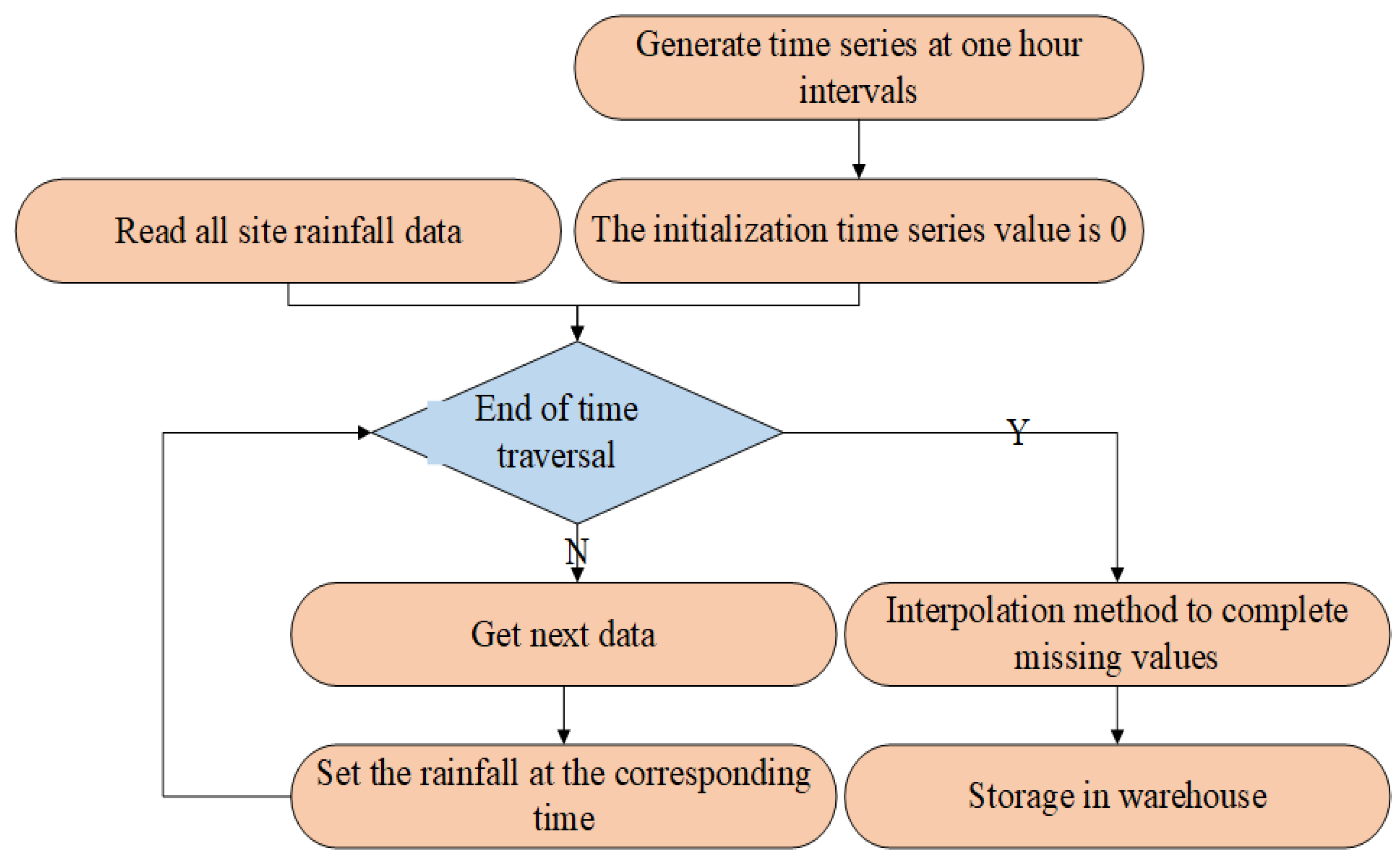
There is also a lack of rainfall data, so inverse distance weighting algorithm is used to complete the missing value. The rainfall at the missing sites was estimated using the distance $d_i$ between the sites and the rainfall at the k adjacent sites as a prior condition. If the rainfall of the missing station is $x^i$, the calculation principle is as shown in Formula (2). For the i-th participating station, the weight value $w_i$ is calculated as shown in Formula (3), which shows an inverse relationship with the square of the distance between the stations, which is also in line with the actual situation.

$$x_{}{}^{\prime }=\sum _{i=1}^k{w}_i{x}_i$$

(2)

$$w_i=\frac{d_i^{-2}}{{\displaystyle \sum _{j=1}^k}{d}_j^{-2}}$$

(3)

After defining the algorithm of rainfall data completion, we design the process as shown in Figure 5 for rainfall data preprocessing.

2.1.3. The Extraction of Remote Sensing Image Information

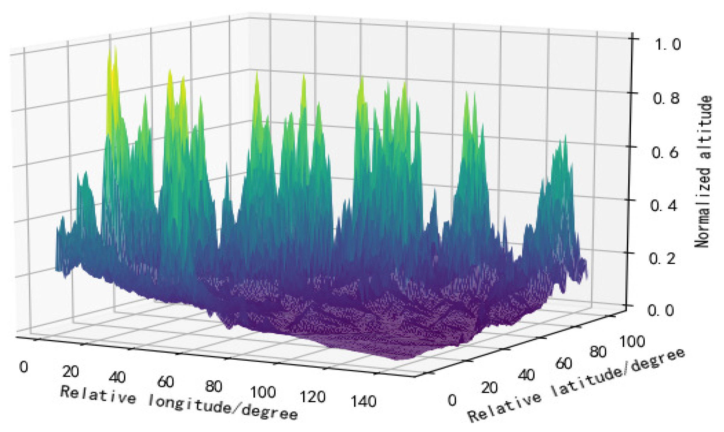
In the construction of the GAT digraph, the convergence direction between two different nodes is determined by the flow direction of the river. According to the laws of physics, the flow in natural rivers is from high to low. Remote sensing images contain a variety of information such as elevation, landform, slope, etc. Therefore, ArcGIS is used to extract digital elevation data from remote sensing images in target basin.

For digital elevation data, it is mainly used to determine the topographic relationship between sites, thereby determining the adjacency relationship between the sites and generating an adjacency matrix. The 3D visualization of the digital elevation information in this area is shown in Figure 6.

2.2. Model Description

In this chapter, the structure and principles of GAT and LSTM networks are explained. Based on the combination of the two structures, the whole structure of the space-time feature fusion network and the settings of super-parameters are proposed.

2.2.1. Graph Neural Network

CNN (Convolutional neural networks) networks and RNN (Recurrent neural networks) can only be used to process data in Euclidean space. In contrast, data in non-Euclidean space, such as social network information, chemical molecular structure, etc. in the traditional scheme cannot do anything. With the introduction of graph neural network, it marks the extension of deep learning technology in non-Euclidean space.

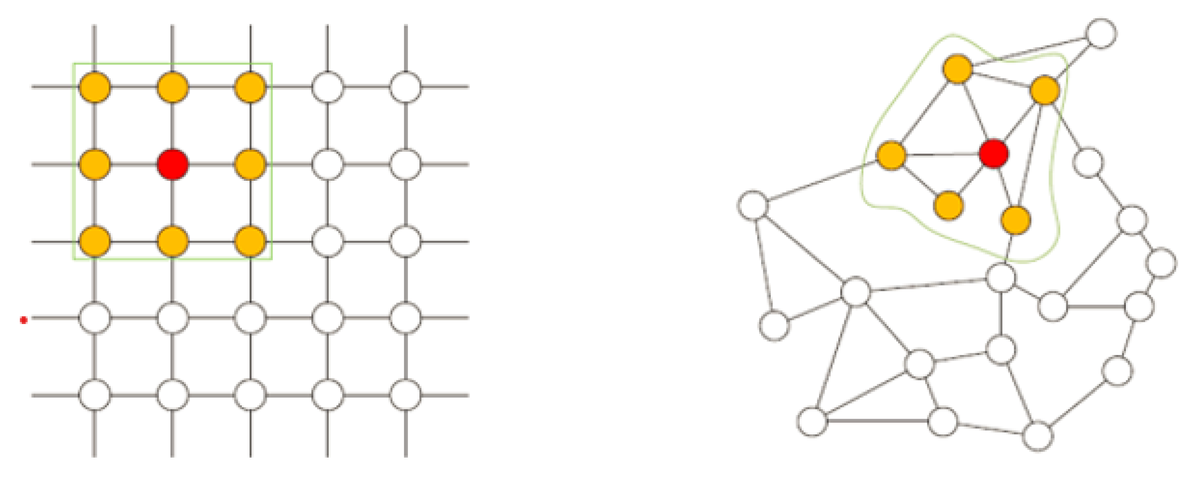
As far as the analyzable problems are concerned, the GNN (graph neural network) covers the analysis domain of CNN and RNN [31]. The problems that CNN and RNN can solve can also be reasonably modeled by using the graph neural network. In CNN, the convolution kernel structure is used. The value of the center pixel node is weighted and summed by the value of the surrounding pixels, and all the pixels in the coverage range of the convolution kernel are considered to be the neighbors of the center pixel. If we consider the relationship between adjacent pixels more carefully and remove the unnecessary connection relationship, the original data will become non-Euclidean data, which cannot be analyzed by CNN, but GNN can effectively model non-Euclidean data. Figure 7 shows Euclidean data and non-Euclidean data.

In the field of flood forecasting, the data of different rainfall stations represent the rainfall information of different areas. The rainfall in different areas mainly affects the flow of downstream hydrological stations through the convergence of the river network. According to the convergence process of the river and the connection relationship between the stations, the rainfall in different areas can be described as a complex graphic structure and analyzed by GNN.

2.2.2. Graph Attention Mechanisms

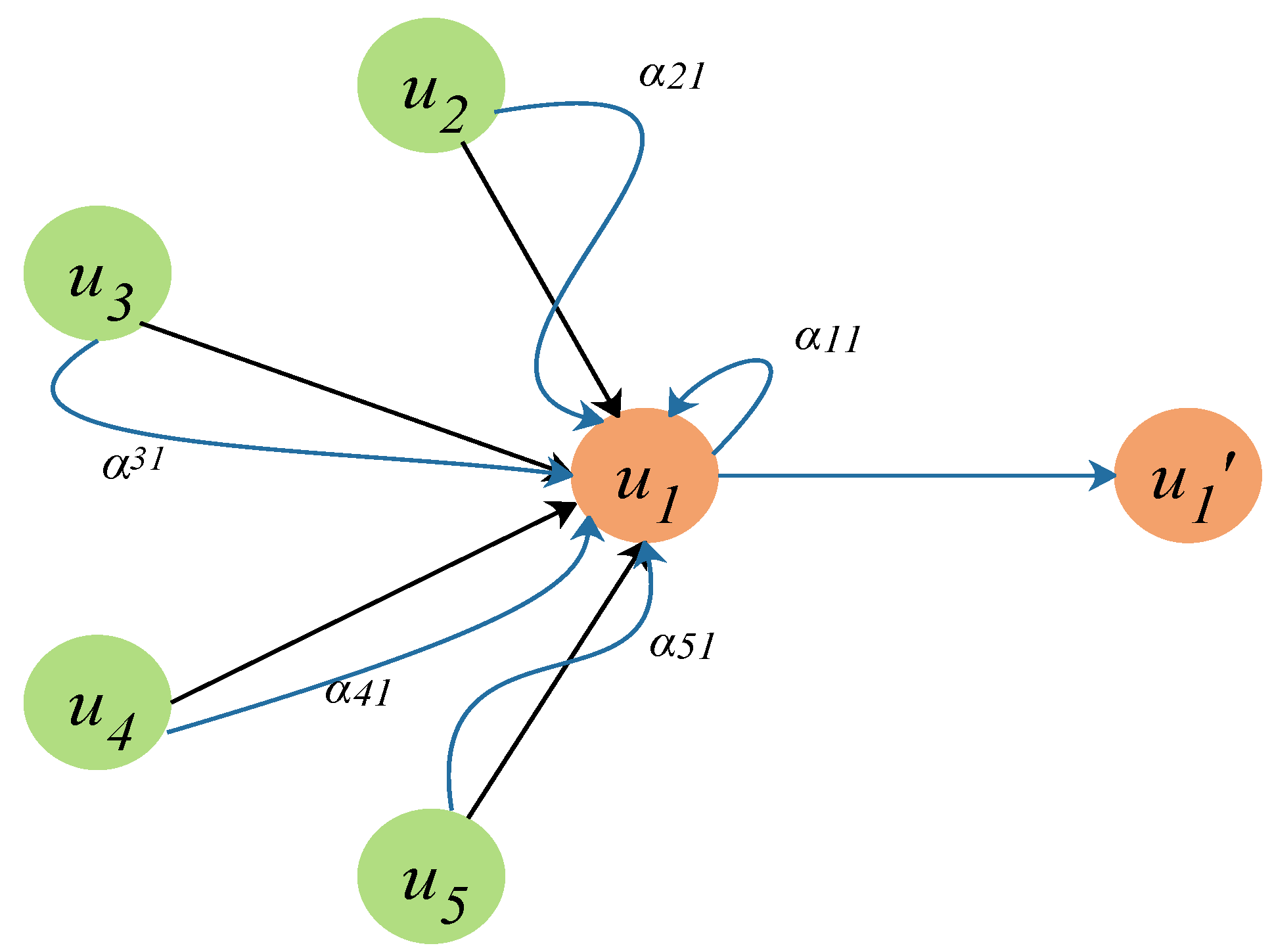
According to the network classification scheme proposed by Zonghan Wu [32] and others in the survey of graph neural networks, graph attention mechanism belongs to the solution based on spatial domain in graph convolution network [33], which can analyze and process data in both digraph and undirected graph formats. The essence of this method is to collect weighted k-level neighborhood rainfall information of each station in the rainfall map data. The input rainfall map signal is u, and the calculated result is $u{}^{\prime }$. The calculation principle is shown in Formula (4). Figure 8 shows a visual representation of this.

$$u_j{}^{\prime }=\sigma (\sum _{i=1}^N{\alpha }_{ij}{u}_i)$$

(4)

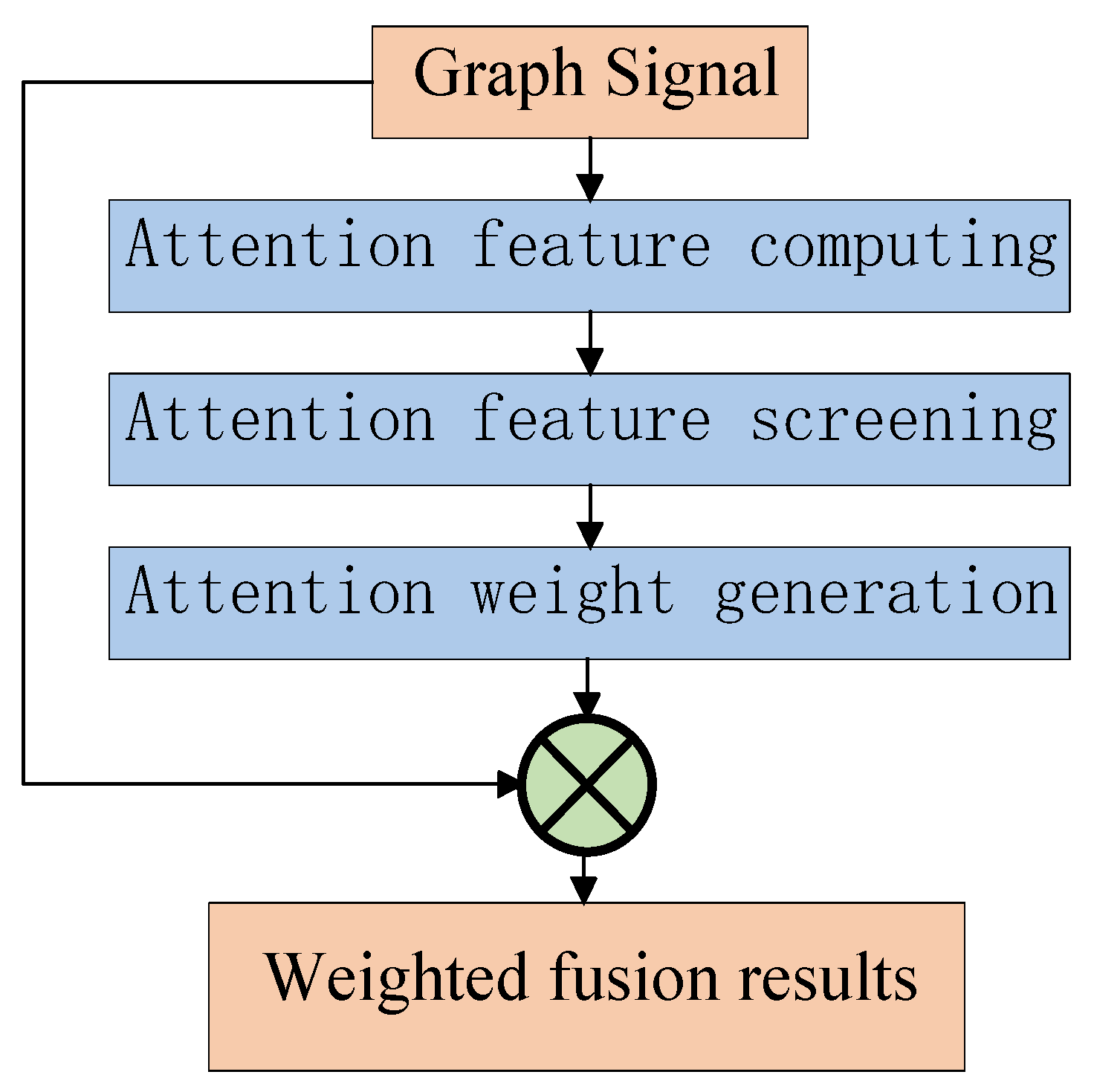
In this paper, a single-head attention mechanism based on first-order neighbors is used. That is, only the first-order neighbors are aggregated, and only the attention weights are calculated once. The overall calculation process is shown in Figure 9.

This paper uses the inner product of two rainfall data vectors to calculate the attention characteristics of each station in the original rainfall map. Since only the first-order neighborhood rainfall features are aggregated, it is necessary to first filter the attention feature vectors. Only the attention features of the neighboring sites are retained, and then the attention weights are generated according to the selection. Finally, the features are weighted and aggregated according to Formula (4).

Let the original rainfall chart signal matrix be U, where each row $u_i$ represents the rainfall information of the $ist$ station, according to Formula (5); it can get the inner product matrix W of each station and all other stations. The $w_{ij}$ represents the first and two sites ($i,j$) of the inner product results.

$$W=U{U}_{}^T$$

(5)

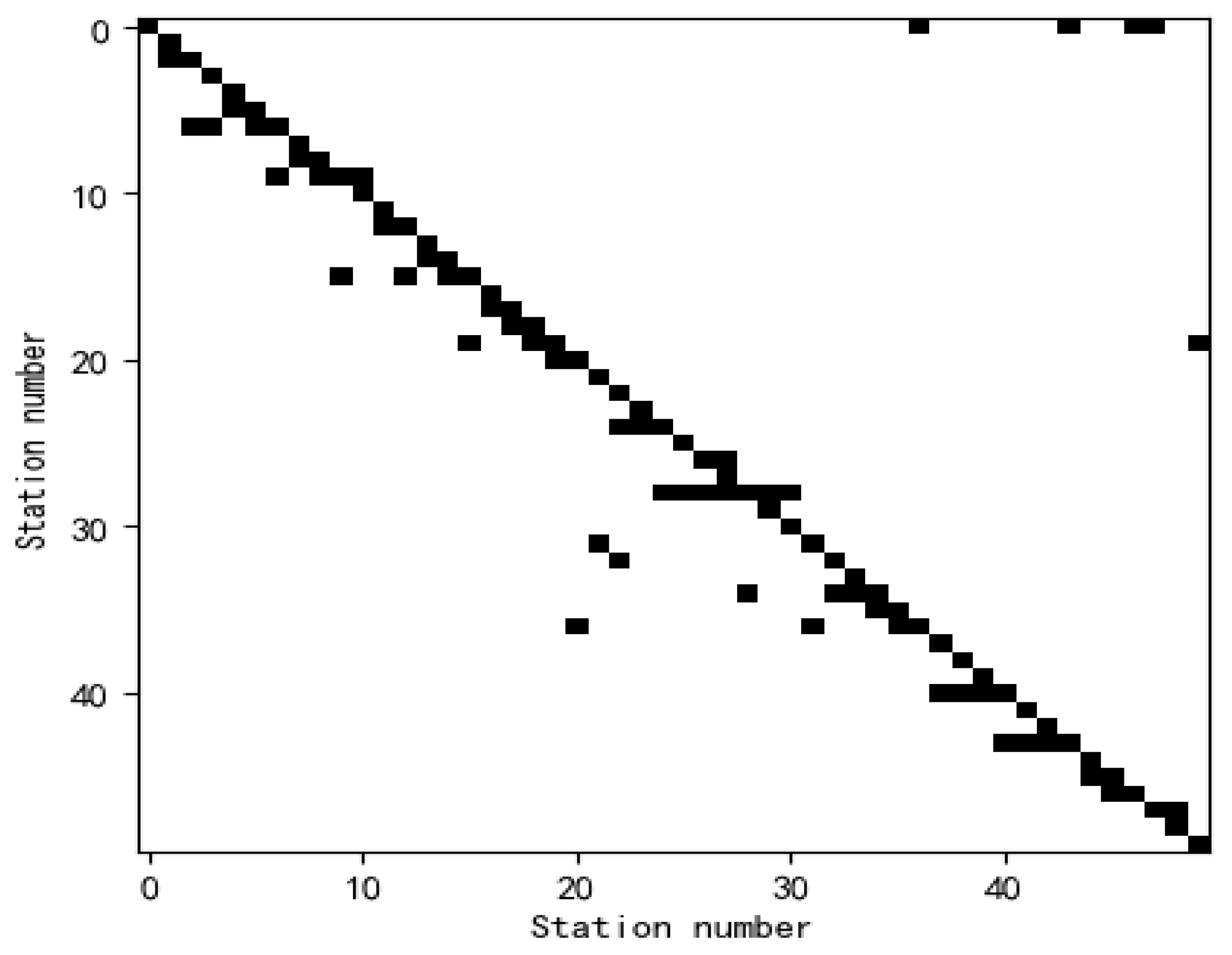
To filter the attention characteristic matrix W, we need to use the adjacency matrix A between nodes. In this study, 50 rain gauge stations are abstracted as nodes. The river channels connecting rainfall stations are abstracted as edges. According to the digital elevation information extracted from remote sensing images of the target basin, the direction of the edge is determined according to the topography. The spatial distribution of rainfall in the area is abstracted into a directed graph and described by an adjacency matrix. The definition of the elements of the adjacency matrix is shown in Formula (6). If the rainfall from the site i can converge to the site j, the element $a_{ij}$ is 1. Figure 10 shows a two-dimensional visualization of the adjacency matrix, where black blocks correspond to non-zero values in the matrix.

$${\alpha }_{ij}=\left\{\begin{array}{ccc}1& & if(i->j)\\ 0& & else\end{array}\right.$$

(6)

After the adjacency matrix is obtained, the eigenvalues $W^{{}^{\prime }}$ are filtered using the Jacques Hadamard product shown in Formula (7).

$$W^{{}^{\prime }}=W·A$$

(7)

As shown in Formula (8), each column of the matrix eigenvalues vector weight was generated by the matrix $W^{{}^{\prime }}$.

$$W_j^{{}^{″}}=\frac{exp\left(w_j^{{}^{\prime }}\right)}{{\sum }_{i}exp\left(w_i^{{}^{\prime }}\right)}$$

(8)

Finally, the weighted fusion graph signal is generated based on Formula (4). The process is vectorized, as shown in Formula (9).

$$U^{{}^{\prime }}=W^{{}^{″}}U$$

(9)

Each row of the computed matrix represents the weighted fusion result of the node and its first-order neighbors.

2.2.3. LSTM Time-Series Analysis Network

The spatial features of rainfall data are extracted by using the attention mechanism of GAT. This study not only focuses on spatial feature mining but also uses LSTM to mine temporal information of rainfall feature itself.

RNN is a classical model used to process time-series information. However, because it has no loss of memory, the chain rule is too long, and the gradient disappears in the optimization process. To solve this problem, we modify the RNN to form the LSTM network [34].

Compared with the original RNN neurons, the LSTM structure is divided into three logical blocks: forgetting gate, update gate, and output gate [35]. The forgetting gate is used to discard part of the time step information to prevent the gradient from disappearing. The updating gate is used to combine the current time step information with the memory information to generate the new neuron state. The output gate is used to generate the current time output of the neuron.

2.2.4. Space-Time Feature Fusion Model Based on GA-RNN Framework

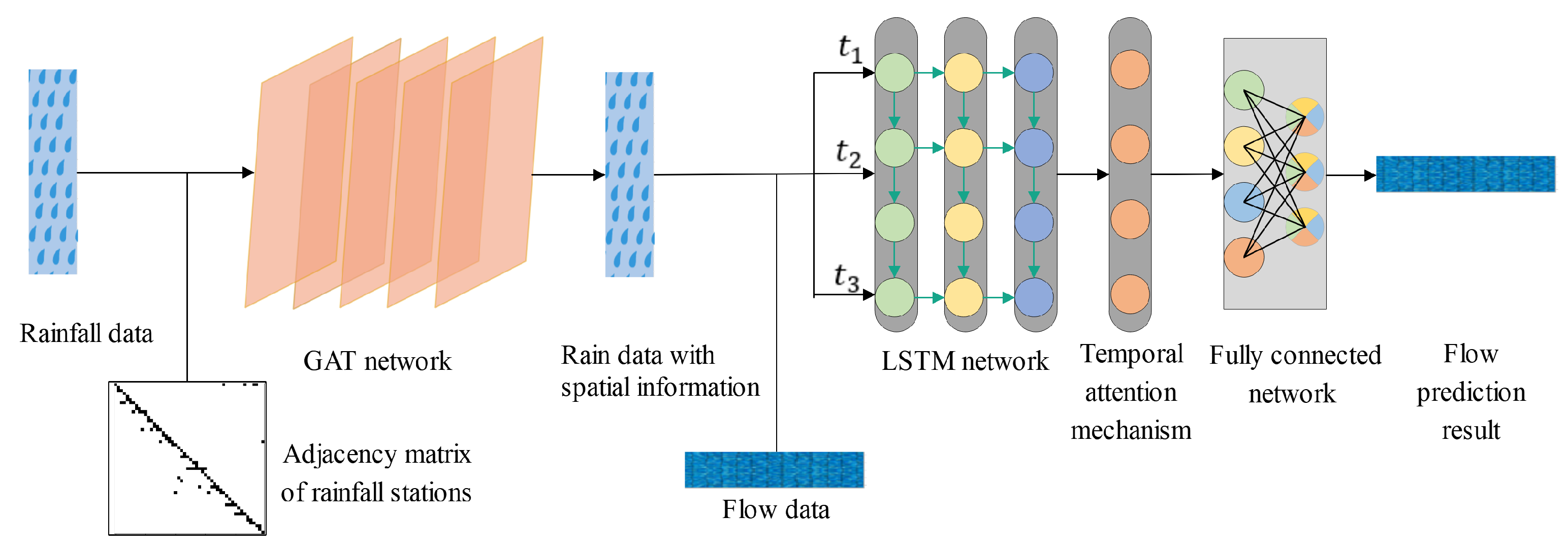
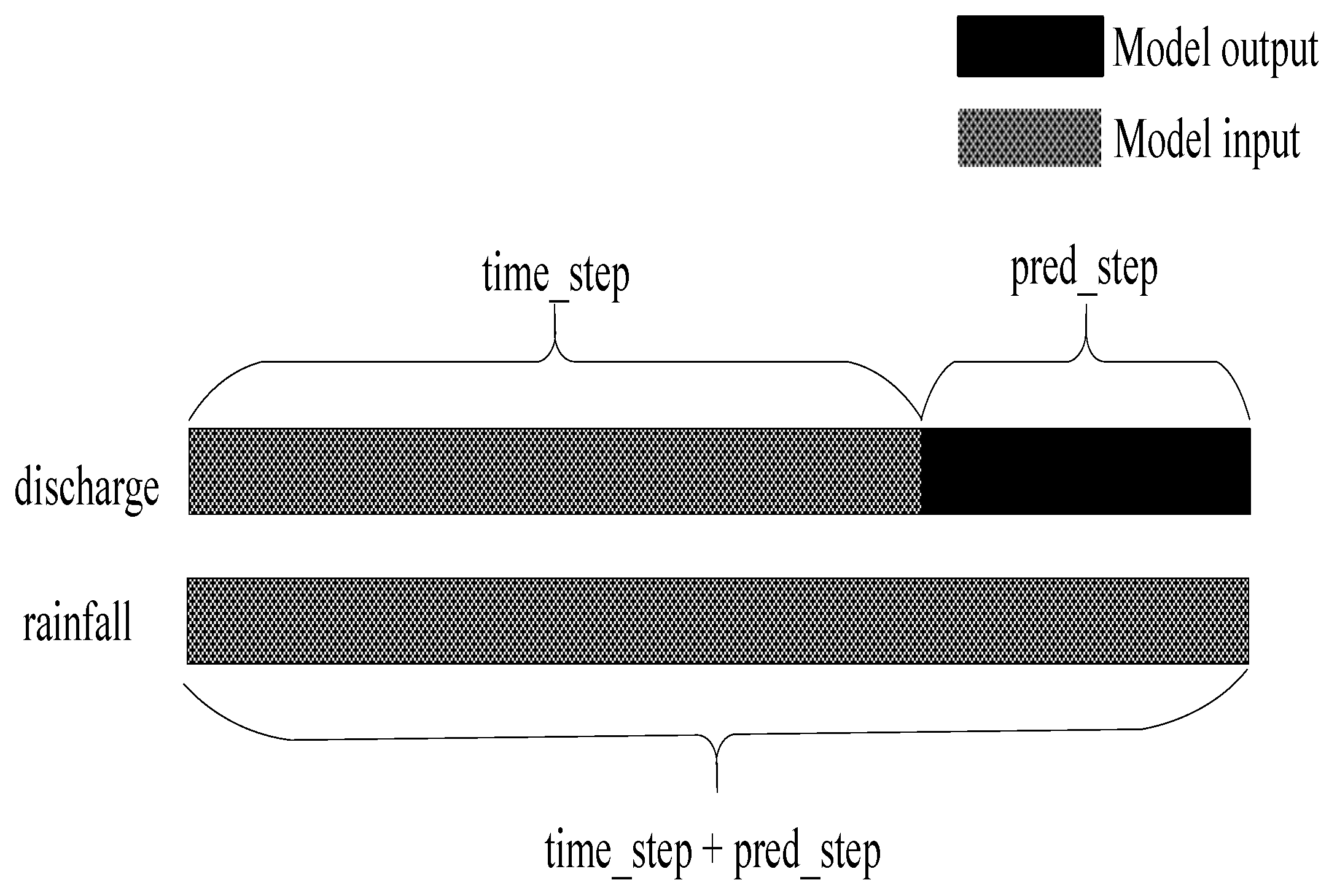
Based on the attention mechanism (GAT) and long-term and short-term memory network (LSTM), the series structure of GAT and LSTM is used to fuse the temporal and spatial characteristics of rainfall data, and the flood flow in the future is predicted and output. As shown in Figure 11, at first, we determine the adjacency between the rainfall stations by extracting the digital elevation information of the remote sensing image of the target basin. Then, through the graph attention mechanism, the spatial information of the rainfall data of the target watershed is extracted, which is specifically expressed as the aggregation relationship of the rainfall data of each station. Then the rainfall data through the GAT network and the flow data of the Xixian hydrological station are input to the LSTM network to complete the flow data prediction of the Xixian hydrological station. In this paper, the time_step is used to represent historical discharge data; pred_step is used to represent the flood forecast period. Figure 12 shows the time dependence of a set of input–output structures of the model.

The model takes the rainfall data of the future pred_step hours as the known data, combined with the rainfall data of the past time_step hours as the input of rainfall information. At the same time, the historical time_step hour flood discharge data is used as the input of historical flood information. Finally, the flood discharge data of the next pred_step hours and the output are predicted.

GAT network is composed of multi-layer graph attention mechanism operation layers, which are used to extract spatial features of rainfall map data.

The LSTM network further extracts time-series information from the rainfall distribution information obtained by the GAT network analysis. A temporal attention mechanism is added to the output layer of LSTM to improve prediction accuracy. Finally, input the output of the LSTM network into the fully connected network for numerical fitting and output the flood flow prediction results. The parameters of each layer of the GAT network and the fully connected network [36] are recorded in

Table 3. GA-RNN parameters of each layer.

Network Layer Name	Parameters of Each Layer
GAT_Layer1	[1,100]
GAT_Layer2	[100,80]
GAT_Layer3	[80,60]
GAT_Layer4	[60,40]
GAT_Layer5	[40,30]
Dense_Layer1	50
Dense_Layer2	40
Dense_Layer3	pred_step

. Furthermore, the number of neurons in each layer of the LSTM network is recorded in

Table 4. Neuron parameters of rainfall LSTM analysis network.

Network Layer Name	Number of Neurous
LSTM_Layer1	50
LSTM_Layer2	30
LSTM_Layer3	10

.

3. Model Training and Effect Demonstration

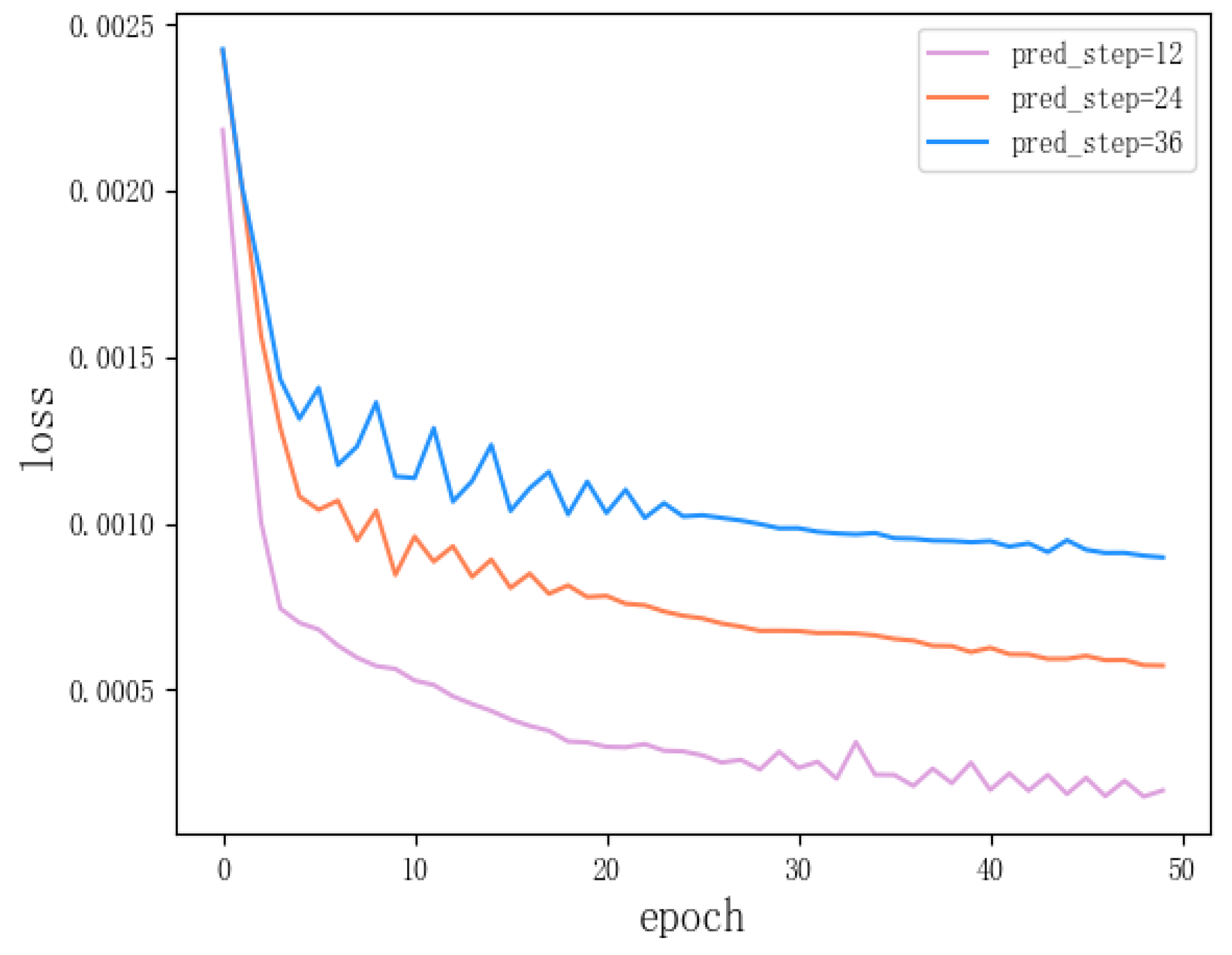
Before the experiment, 50 rainfall stations with data volume of more than 26,000 in 5 years were selected. The rainfall data of 50 rainfall stations and the flow data of the Xixian hydrological station are used to construct the train set. The data of the train set are from 2012 to 2017. The training parameters are set as shown in

Table 5. GA-RNN training parameter setting.

Name of Training Parameter	Parameter Value
epochs	50
batch size	40
optimizer	Adam
loss function	MSE
learning rate	0.005

. The loss function curve of the training process is shown in Figure 13. For the model, the more data there is, the more accurate the prediction result is. The minimum data set to properly adjust the neural network is that each station has more than 60% of the hourly rainfall and flow data within 3 years (that is, the amount of data at each site should exceed 3 × 365 × 24 × 60% = 15,768).

3.1. Comparison of Full-Year Forecasts

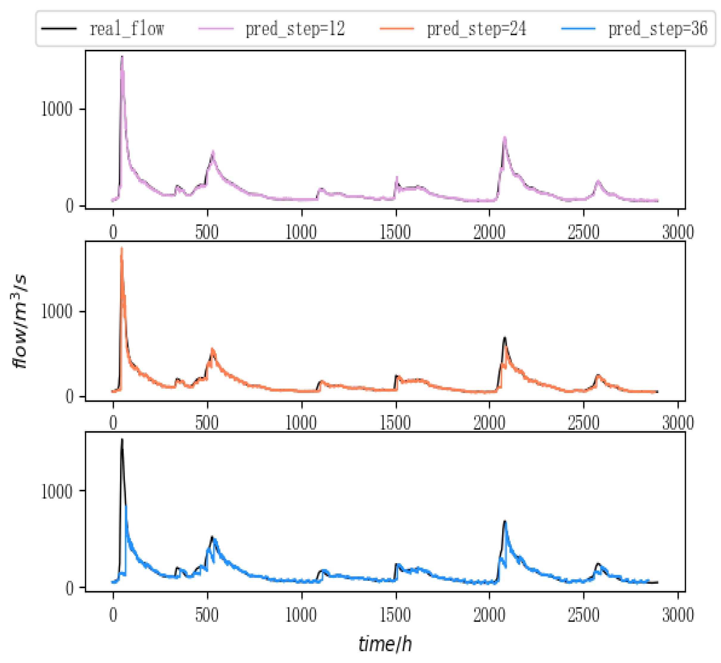
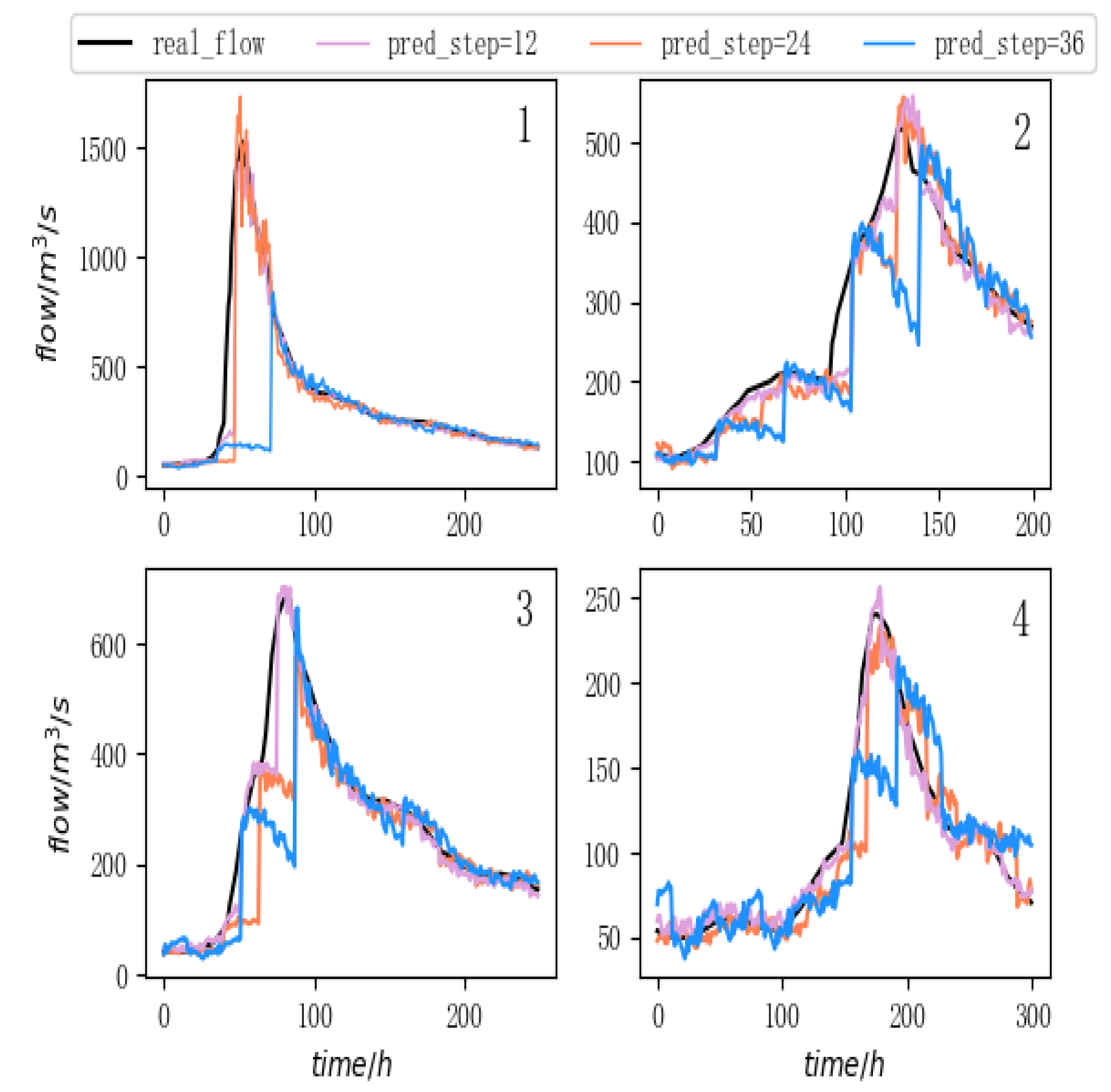
Using the successfully trained model, a forecasting experiment was carried out in the flood season of 2018, and 12-h, 24-h, and 36-h forecast models were established respectively. Figure 14 compares the forecast and actual flow curves for the three forecast periods. According to the calculation principles of Formulas (10) and (11), the root means square error (RMSE) and coefficient of determination ($R^2$) of the model results in the three forecast periods are calculated, as shown in

Table 6. Comparison of numerical effect of flood season discharge forecast in 2018.

Pred_STEP (h)	RMSE (m${}^3/$s)	${\mathit{R}}^2$
12	40.99	0.93
24	57.39	0.86
36	118.26	0.41

. The RMSE can reflect the overall fit between the predicted curve and the actual curve. The smaller the value, the smaller the error, and the higher the prediction accuracy of the model. The $R^2$ is a statistical indicator used to reflect the reliability of the dependent variable in the regression model. To a certain extent, when the value of the $R^2$ is close to 1, the trained model is more reliable and real. The closer the model is to zero, the worse it looks.

$$RMSE=\sqrt{\frac{1}{m}\sum _{i=1}^m{(y_i-{\widehat{y}}_i)}^2}$$

(10)

$$R^2=1-\frac{{\displaystyle \sum _{i=1}^m}{\left(\widehat{yi-y_i}\right)}^2}{{\displaystyle \sum _{i=1}^m}{(y_i-\frac{1}{m}{\displaystyle \sum _{j=1}^m}{y}_i)}^2}$$

(11)

3.2. Analysis of Flood Process Index

According to the flood forecasting specification [37] stipulated by the Ministry of Water Resources of the People’s Republic of China, the allowable error range of flood peak forecast accuracy is 20%, and the allowable error of flood peak arrival time is 30%. According to this regulation, four typical flood events in 2018 are selected for index evaluation. The curve fitting results are shown in Figure 15. The prediction errors of flood peak, arrival time, and preliminary evaluation results are shown in

Table 7. Flood process precision index.

Pred_STEP	Flood Number	Peak Error	Y/N	Time Error	Y/N
12	1	2.8%	Y	7.7%	Y
	2	4.1%	Y	2.3%	Y
	3	2.4%	Y	1.3%	Y
	4	3.0%	Y	3.5%	Y
24	1	12.3%	Y	1.9%	Y
	2	7.7%	Y	6.3%	Y
	3	3.3%	Y	10.0%	Y
	4	6.8%	Y	3.5%	Y
36	1	45.2%	N	40.4%	N
	2	7.8%	Y	13.3%	Y
	3	15.3%	Y	11.3%	Y
	4	10.6%	Y	12.2%	Y

.

3.3. Superiority Discrimination of Space-Time Fusion Model

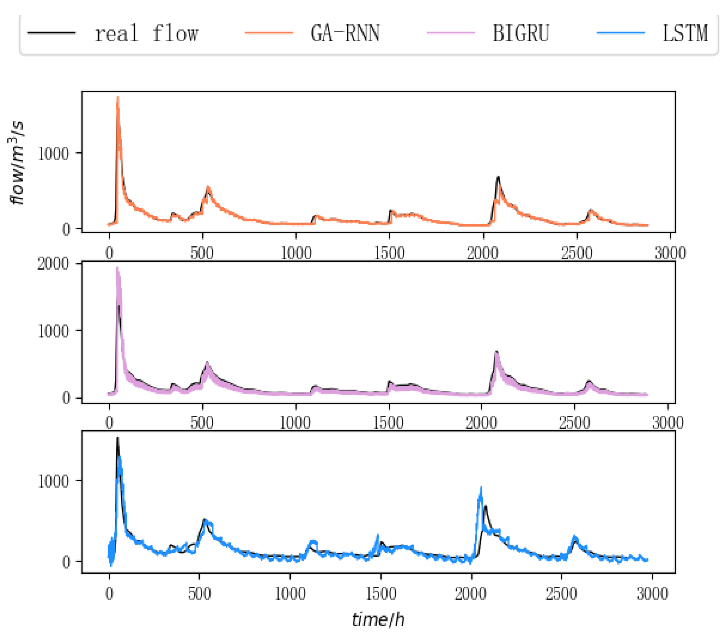
To verify the superiority of the proposed spatiotemporal feature fusion scheme, the GAT network module in GA-RNN is removed, and the time-series analysis network model based on LSTM structure is obtained. In addition, we have also conducted comparative experiments with the BIGRU model proposed by Liang Xiaoxu et al.

The train set and test set of the three models are consistent. At the same time, one sets the forecast period to 24-h and the training parameters of the two models according to Table 5. Figure 16 shows the comparison between the predicted results of the two models and the actual flow.

Table 8. GA-RNN, comparison of numerical effects of LSTM flow prediction.

Model Name	RMSE (m${}^3/$s)	${\mathit{R}}^2$
GA-RNN	57.39	0.86
BIGRU	70.86	0.78
LSTM	83.69	0.70

records their performance in terms of RMSE and $R^2$.

3.4. Evaluation of Model Forecast Grade

According to [37] and Formula (12), the qualified rate of forecast result of the model is calculated. In Formula (12), N is the total number of forecasts, and M is the number of qualified forecasts.

$$QR=\frac{M}{N}\times 100\%$$

(12)

The comprehensive qualified rate and the $R^2$ can be used to evaluate the grade of the flood forecasting model, and the evaluation rules are shown in

Table 9. Evaluation table of model forecast grade.

Model Grade	QR (%)	${\mathit{R}}^2$
Class A	$QR\ge 85.0$	$R^2\ge 0.90$
Class B	$85.0>QR\ge 70.0$	$R^2\ge 0.70$
Class C	$70.0>QR\ge 60.0$	$R^2\ge 0.50$

[37].

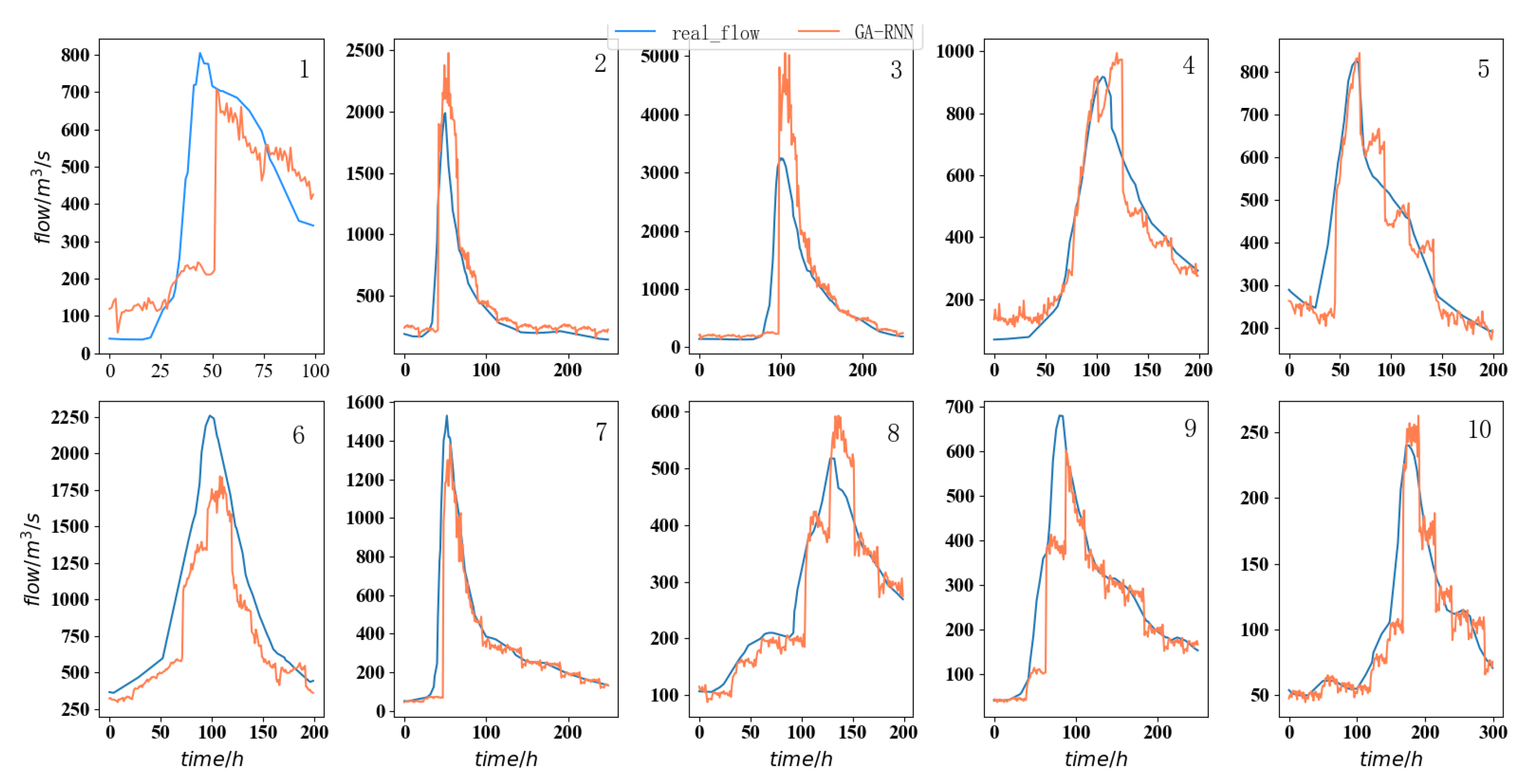
By dividing the train set and the test set many times, this paper has counted ten typical flood processes in history and modeled them with a 24-h forecast period.

Figure 17 shows the prediction results of GA-RNN in ten historical floods. Figure 17 shows the prediction results of GA-RNN in ten historical floods. According to the discriminant rules shown in Table 9, the predicted peak value and peak arrival time error of each flood are calculated respectively, and then the model is classified. The results are shown in

Table 10. Comparison of historical flood forecasting indexes and model rating.

NO	Peak Error	Y/N	Time Error	Y/N	QR	Grade
1	12.2%	Y	2.8%	Y	80%	Class B
2	24.6%	N	5.0%	Y
3	55.5%	N	5.9%	Y
4	8.4%	Y	13.2%	Y
5	2.1%	Y	4.5%	Y
6	18.4%	Y	10.2%	Y
7	9.8%	Y	7.7%	Y
8	14.6%	Y	6.3%	Y
9	11.6%	Y	10.0%	Y
10	9.4%	Y	10.5%	Y

.

4. Discussion

As shown in Table 6 and Figure 14, in the annual forecast results of the model, it can be seen from the curve fitting effect that the curve fitting degree decreases with the increase of the forecast period, especially during the flood peak forecast period. When the prediction time becomes longer, the prediction difficulty of the model also increases. For the same time_step, the historical data obtained by the model is the same, but as the prediction length of the model increases, the difficulty of the model prediction also increases. When predicting data that is farther away from historical data, there may be a large error between the information obtained by the model and the real information. Therefore, the accuracy of the model will also decrease. In practical applications, a shorter forecast period usually requires higher forecast accuracy. From this point of view, the model conforms to the characteristics of the actual flood forecasting model.

As shown in Table 7 and Figure 15, in the 12 h and 24-h forecast period, the GA-RNN model achieved the error standard for the prediction of the key indicators of the four floods. When the forecast period increases to 36 h, the first flood forecast index becomes worse, which does not conform to the error criterion. However, the results of the other three flood forecasts still meet the standard. The differences between the first flood and the other three floods are analyzed and compared. When the first flood reaches the peak value, the flood discharge exceeds 1000 m${}^3/$s, which has the characteristics of high peak value and rapid change. This large scale and fast change make the model less effective in a long prediction period. This may be because the model learns less for this type of data.

As shown in Table 8 and Figure 15, from the perspective of the predicted discharge curve, the GA-RNN model based on spatiotemporal feature fusion is superior to the LSTM network based on time-series analysis, especially when a flood occurs. It can predict flood peak and arrival time well. The RMSE of the GA-RNN model is 13.47% lower than that of the BIGRU model, and $R^2$ is 8% higher. The RMSE of the GA-RNN model is 26.3% lower than the LSTM model, and the $R^2$ is 16% higher. Compared with the LSTM model, the BIGRU model can comprehensively consider the context information of the input sequence, so the prediction accuracy is improved, but the effect is worse than the GA-RNN model. Comparative experiments show that the spatial feature extraction of rainfall data is very important, and the spatiotemporal feature fusion scheme is superior to the traditional pure time-series analysis model in prediction accuracy.

As shown in Table 10 and Figure 17, in terms of flood process prediction, the GA-RNN model can accurately fit the real flow curve, and according to the discriminant rules shown in Table 9, the GA-RNN model flood forecast qualification rate can reach 80%, which can be assessed if it is a B-level model. Only floods #2 and #3 exceed the allowable error. The reason for the over-prediction of floods #2 and #3 is that the flow of these two floods is too large. This large-scale and rapid change make the model less effective in a long prediction period, which may be due to the lack of such data in the training set. Compared with floods #2 and #3, the rainfall of floods #1 and #6 is relatively small and gentle, and the peak flow rate is slower. Therefore, the prediction curve of the model is relatively flat, resulting in the prediction peak value of the model being lower than the true value. Therefore, this model can be considered for actual production. Due to the limited training data of the model during the experiment, especially the lack of heavy rainfall data, the effect of the model is limited. If there are more flood data, it is predicted that the effect of the model will be better.

5. Conclusions

Aiming at the current situation of insufficient rainfall spatial feature mining in the existing flood forecasting data-driven models, this paper proposes a GA-RNN space-time feature fusion model. The 50 rainfall stations are abstracted as nodes, and the rivers connected between rainfall stations are abstracted as edges. Digital elevation information from remote sensing images is extracted to determine the direction of the edge. The rainfall data is described by graph data, and the graph attention mechanism is introduced for spatial feature analysis. Through the experiment of flood forecasting, it can be found that over 90% of the forecast results of the GA-RNN model meet the standard under different forecast periods, and the shorter the forecast periods, the higher the accuracy. At the same time, for the ten historical floods, more than 80% of the predicted results also met the standard. According to the hydrological evaluation criteria, the GA-RNN model is assessed as a Class B flood forecasting model. In the model comparison experiment, the RMSE of the GA-RNN model is 13.47% lower than that of the BIGRU model, and $R^2$ is 8% higher. The RMSE of the GA-RNN model is 26.3% lower than the LSTM model, and the $R^2$ is 16% higher. It shows that the prediction accuracy of the model has been significantly improved after using remote sensing images to add the spatial feature extraction of rainfall data. However, when the flood peak discharge is high and the speed of change is fast, the prediction error of the model is relatively large. By increasing the proportion of this situation in the train set, perhaps the accuracy can be further improved. Besides, the GA-RNN model only considers rainfall and flow characteristics. If evapotranspiration, weather, vegetation, and other characteristics that affect flood flow can be considered, the accuracy of the model may be more improved. At the same time, as we all know, machine learning-based models are very dependent on data, and the quality of the data directly affects the results of the model. For many areas where the collection of hydrological information is difficult, the use of the model faces great difficulties. The universality of the model is relatively poor, especially because the model needs to obtain the digital elevation information of the area.

References

1. Dottori, F.; Salamon, P.; Bianchi, A.; Alfieri, L.; Hirpa, F.A.; Feyen, L. Development and evaluation of a framework for global flood hazard mapping. Adv. Water Resour. 2016, 94, 87–102. [Google Scholar] [CrossRef]
2. Löwe, R.; Urich, C.; Domingo, N.D.F.S.; Mark, O.; Deletic, A.; Arnbjerg-Nielsen, K. Assessment of Urban Pluvial Flood Risk and Efficiency of Adaptation Options Through Simulations—A New Generation of Urban Planning Tools. J. Hydrol. 2017, 550, 355–367. [Google Scholar] [CrossRef] [Green Version]
3. Wannous, C.; Velasquez, G. United Nations Office for Disaster Risk Reduction (UNISDR)—UNISDR’s Contribution to Science and Technology for Disaster Risk Reduction and the Role of the International Consortium on Landslides (ICL) Open image in new window. In Workshop on World Landslide Forum; Springer: Cham, Switzerland, 2017; pp. 109–115. [Google Scholar]
4. Doocy, S.; Daniels, A.; Packer, C.; Dick, A.; Kirsch, T.D. The human impact of earthquakes: A historical review of events 1980–2009 and systematic literature review. PLoS Curr. 2013, 5, 1808–1815. [Google Scholar] [CrossRef]
5. Jonkman, S.N. Global Perspectives on Loss of Human Life Caused by Floods. Nat. Hazards 2005, 34, 151–175. [Google Scholar] [CrossRef]
6. Zhao, M.; Hendon, H.H. Representation and prediction of the Indian Ocean dipole in the POAMA seasonal forecast model. Q. J. R. Meteorol. Soc. 2009, 135, 337–352. [Google Scholar] [CrossRef]
7. Cea, L.; Garrido, M.; Puertas, J. Experimental validation of two-dimensional depth-averaged models for forecasting rainfall-runoff from precipitation data in urban areas. J. Hydrol. 2010, 382, 88–102. [Google Scholar] [CrossRef]
8. Costabile, P.; Costanzo, C.; Macchione, F. Comparative analysis of overland flow models using finite volume schemes. J. Hydroinformat. 2012, 14, 122–135. [Google Scholar] [CrossRef] [Green Version]
9. Xia, X.; Liang, Q.; Ming, X.; Hou, J. An efficient and stable hydrodynamic model with novel source term discretization schemes for overland flow and flood simulations. Water Resour. Res. 2017, 53, 3730–3759. [Google Scholar] [CrossRef]
10. Costabile, P.; Macchione, F. Enhancing river model set-up for 2-D dynamic flood modelling. Environ. Model. Softw. 2015, 67, 89–107. [Google Scholar] [CrossRef]
11. Kim, B.; Sanders, B.F.; Famiglietti, J.S.; Guinot, V. Urban flood modeling with porous shallow-water equations: A case study of model errors in the presence of anisotropic porosity. J. Hydrol. 2015, 523, 680–692. [Google Scholar] [CrossRef] [Green Version]
12. van den Honert, R.C.; McAneney, J. The 2011 Brisbane Floods: Causes, Impacts and Implications. Water 2011, 3, 1149–1173. [Google Scholar] [CrossRef] [Green Version]
13. Wang, X.; Ren, X.; Qiu, C.; Cao, Y.; Taleb, T.; Leung, V.C.M. Net-in-AI: A Computing-Power Networking Framework with Adaptability, Flexibility, and Profitability for Ubiquitous AI. IEEE Netw. 2021, 35, 280–288. [Google Scholar] [CrossRef]
14. Prakash, O.; Sudheer, K.; Srinivasan, K. Improved higher lead time river flow forecasts using sequential neural network with error updating. J. Hydrol. Hydromech. 2014, 62, 60–74. [Google Scholar] [CrossRef]
15. Shu, C.; Ouarda, T. Regional flood frequency analysis at ungauged sites using the adaptive neuro-fuzzy inference system. J. Hydrol. 2008, 349, 31–43. [Google Scholar] [CrossRef]
16. Ashrafi, M.; Chua, L.H.C.; Quek, C.; Qin, X. A fully-online neuro-fuzzy model for flow forecasting in basins with limited data. J. Hydrol. 2017, 545, 424–435. [Google Scholar] [CrossRef]
17. Yu, P.S.; Yang, T.C.; Chen, S.Y.; Kuo, C.M.; Tseng, H.W. Comparison of random forests and support vector machine for real-time radar-derived rainfall forecasting. J. Hydrol. 2017, 552, 92–104. [Google Scholar] [CrossRef]
18. Yuanhao, X.; Qiang, W.; Changqing, L.; Youqian, C.; ZHANG, L.; Guang, R.; Caihong, H. Simulation of the flood process in the middle reaches of the Yellow River by a long-short term memory (LSTM) neuro network. J. Beijing Norm. Univ. (Nat. Sci. Ed.) 2020, 56, 387–393. [Google Scholar]
19. Dtissibe, F.Y.; Ari, A.; Titouna, C.; Thiare, O.; Gueroui, A.M. Flood forecasting based on an artificial neural network scheme. Nat. Hazards 2020, 104, 1211–1237. [Google Scholar] [CrossRef]
20. Lv, N.; Liang, X.; Chen, C.; Zhou, Y.; Li, J.; Wei, H.; Wang, H. A long Short-Term memory cyclic model with mutual information for hydrology forecasting: A Case study in the xixian basin. Adv. Water Resour. 2020, 141, 103622. [Google Scholar] [CrossRef]
21. Chen, C.; Liu, X.; Qiu, T.; Sangaiah, A.K. A short-term traffic prediction model in the vehicular cyber–physical systems. Future Gener. Comput. Syst. 2017, 105, 894–903. [Google Scholar] [CrossRef]
22. Wan, S.; Ding, S.; Chen, C. Edge computing enabled video segmentation for real-time traffic monitoring in internet of vehicles. Pattern Recognit. 2022, 121, 108146. [Google Scholar] [CrossRef]
23. Wang, L.; Li, M.; Fang, X.; Nappi, M.; Wan, S. Improving random walker segmentation using a nonlocal bipartite graph. Biomed. Signal Process. Control 2022, 71, 103154. [Google Scholar] [CrossRef]
24. Lv, N.; Chen, C.; Qiu, T.; Sangaiah, A.K. Deep Learning and Superpixel Feature Extraction Based on Contractive Autoencoder for Change Detection in SAR Images. IEEE Trans. Ind. Inform. 2018, 14, 5530–5538. [Google Scholar] [CrossRef]
25. Qiao-r, L. Short-term Traffic Flow Forecasting Model Based on SVM and Adaptive Spatio-Temporal Data Fusion. J. Beijing Univ. Technol. 2015, 41, 597–602. [Google Scholar]
26. Zeng-qiang, M. License Plate Character Recognition Based on Convolutional Neural Network LeNet-5. Comput. Simul. 2010, 22, 638–641. [Google Scholar]
27. Ding, Y.; Zhu, Y.; Feng, J.; Zhang, P.; Cheng, Z. Interpretable spatio-temporal attention LSTM model for flood forecasting. Neurocomputing 2020, 403, 348–359. [Google Scholar] [CrossRef]
28. Soltani, K.; Ebtehaj, I.; Amiri, A.; Azari, A.; Bonakdari, H. Mapping the Spatial and Temporal Variability of Flood Susceptibility Using Remotely Sensed Normalized Difference Vegetation Index and the Forecasted Changes in the Future. Sci. Total Environ. 2021, 770, 145288. [Google Scholar] [CrossRef]
29. Gudiyangada, T.; Piralilou, S.T.; Gholamnia, K.; Ghorbanzadeh, O.; Blaschke, T. Flood Susceptibility Mapping with Machine Learning, Multi-Criteria Decision Analysis and Ensemble Using Dempster Shafer Theory. J. Hydrol. 2020, 590, 125275. [Google Scholar] [CrossRef]
30. Veličković, P.; Cucurull, G.; Casanova, A.; Romero, A.; Liò, P.; Bengio, Y. Graph Attention Networks. arXiv 2017, arXiv:1710.10903. [Google Scholar]
31. Sato, R. A Survey on The Expressive Power of Graph Neural Networks. arXiv 2020, arXiv:2003.04078. [Google Scholar]
32. Wu, Z.; Pan, S.; Chen, F.; Long, G.; Zhang, C.; Philip, S.Y. A comprehensive survey on graph neural networks. IEEE Trans. Neural Netw. Learn. Syst. 2020, 32, 4–24. [Google Scholar] [CrossRef] [PubMed] [Green Version]
33. Duvenaud, D.; Maclaurin, D.; Aguilera-Iparraguirre, J.; Gómez-Bombarelli, R.; Hirzel, T.; Aspuru-Guzik, A.; Adams, R.P. Convolutional networks on graphs for learning molecular fingerprints. arXiv 2015, arXiv:1509.09292. [Google Scholar]
34. Hochreiter, S.; Schmidhuber, J. Long short-term memory. Neural Comput. 1997, 9, 1735–1780. [Google Scholar] [CrossRef]
35. Greff, K.; Srivastava, R.K.; Koutník, J.; Steunebrink, B.R.; Schmidhuber, J. LSTM: A search space odyssey. IEEE Trans. Neural Netw. Learn. Syst. 2016, 28, 2222–2232. [Google Scholar] [CrossRef] [PubMed] [Green Version]
36. Chen, C.; Li, J.; Balasubramaniam, V.; Wu, Y.; Zhang, Y.; Wan, S. Contention Resolution in Wi-Fi 6-Enabled Internet of Things Based on Deep Learning. IEEE Internet Things J. 2021, 8, 5309–5320. [Google Scholar] [CrossRef]
37. Sun, J.; Zhang, J.; Wang, J.; Liang, J. Standard for Hydrological Information and Hydrological Forecasting; China Water and Power Press: Beijing, China, 2000. [Google Scholar]
Figure 1. Locations of the Xixian hydrological station and the main rivers in the target basin.
Remotesensing 13 05023 g001
Figure 2. Distribution of the Xixian hydrological station and rainfall stations in the target basin.
Remotesensing 13 05023 g002
Figure 3. Flow data processing in the Xixian hydrological station.
Remotesensing 13 05023 g003
Figure 4. Comparison of normalized water level-flow curves.
Remotesensing 13 05023 g004
Figure 5. Rainfall treatment process.
Remotesensing 13 05023 g005
Figure 6. Visualization of digital elevation in the target basin.
Remotesensing 13 05023 g006
Figure 7. Euclidean data (left) and non-Euclidean data (right).
Remotesensing 13 05023 g007
Figure 8. Concentration weighted fusion.
Remotesensing 13 05023 g008
Figure 9. Diagram of the attention mechanism operation flow.
Remotesensing 13 05023 g009
Figure 10. Adjacency matrix of the target basin based on directed graph analysis.
Remotesensing 13 05023 g010
Figure 11. GA-RNN space-time feature fusion model structure.
Remotesensing 13 05023 g011
Figure 12. GA-RNN model input–output structure.
Remotesensing 13 05023 g012
Figure 13. GA-RNN training loss curve.
Remotesensing 13 05023 g013
Figure 14. GA-RNN flood season forecast effect comparison in 2018.
Remotesensing 13 05023 g014
Figure 15. Forecast effect of flood process in 2018.
Remotesensing 13 05023 g015
Figure 16. GA-RNN, BIGRU, LSTM flow prediction comparison.
Remotesensing 13 05023 g016
Figure 17. Historical flood forecasting effect.
Remotesensing 13 05023 g017