Geometric-Manifold-Assisted Distributed Navigation Probabilistic Information Fusion Cooperative Positioning Algorithm

Abstract

Positioning information is the cornerstone of a new generation of electronic information technology applications represented by the Internet of Things and smart city. However, due to various environmental electromagnetic interference, building shielding, and other factors, the positioning source can fail. Cooperative positioning technology can realize the sharing of positioning information and make up for the invalid positioning source. When one node in the cooperative positioning network has error, the positioning stability of all nodes in the whole cooperative network will be significantly reduced, but the positioning probability information technology can effectively reduce the impact of mutation error. Based on this idea, this paper proposes an information-geometry-assisted distributed algorithm for probabilistic cooperative fusion positioning (IG-CP) of navigation information. The position information of different types of navigation sources is utilized to establish a probability density model, which effectively reduces the influence of a single position error on the whole cooperative position network. Combined with the nonlinear fitting characteristics of the information geometric manifold, mapping and fusion of the ranging information between cooperative nodes on the geometric manifold surface are conducted to achieve cooperative positioning, which can effectively improve the stability of the positioning results. The proposed algorithm is simulated and analyzed in terms of the node positioning error, ranging error, convergence speed, and distribution of the cooperative positioning network. The simulation results show that our proposed cooperative positioning algorithm can effectively improve the positioning stability and display better positioning performance.

1. Introduction

Cooperative positioning is the core foundation of 5G application technologies such as Internet of Things and smart city. Due to the inherent errors of satellite navigation, inertial navigation, and other navigation methods, some nodes in the cooperative network will have error mutation [1,2,3,4,5,6,7]. It is very important to study the stability of cooperative positioning accuracy. The cooperative position system has received much attention from the research community and has wide applications, such as regional unmanned driving and an unmanned distribution network for urban forests [8,9,10]. Unmanned aerial vehicles (UAVs) need the support of high-stability positioning in the above scenarios; fortunately, the cooperative positioning system has many advantages in improving the stability of positioning accuracy.

Early cooperative positioning technology mainly utilized ranging and direction finding to obtain the positions of nodes. The first generation of cooperative positioning technology mainly carried out the centralized processing of data to achieve navigation and positioning [11,12,13,14,15]. By measuring the distance between the central node and the surrounding nodes, combined with the node’s own positioning information, the positioning information of all nodes could be obtained. When an error occurs at any node, it will affect the whole cooperative positioning network and decrease the stability of positioning accuracy [14]. In a high-interference environment such as the battlefield environment, centralized cooperative positioning is more vulnerable to interference, which leads to the reduction of the positioning stability of all the participating cooperative nodes [15].

On the other hand, the ranging error between cooperative network nodes and their own position error will further affect the stability of positioning, but it is difficult to measure and evaluate these errors [16]. In early cooperative positioning systems, a large number of cooperative nodes did not have positioning ability; thus, high-precision positioning nodes were required as base stations to provide positioning coordinates to achieve the positioning of all cooperative nodes [17,18,19,20,21]. Therefore, the centralized cooperative positioning technology usually ignores the stability of node positioning accuracy. A multisensor data fusion cooperative position (MSDFC) algorithm is proposed in [22]. The cooperative node transfers the positioning data to the central node; then, optimal estimation of the positioning results of all nodes in the whole cooperative network is achieved. A semidefined programming (SDP) method is proposed in [23] to realize cooperative positioning, in which cooperative nodes can achieve high robustness in different topology networks. These methods can effectively improve the positioning accuracy of the participating nodes, but they have higher requirements for ranging and communication performance. In [22,23,24]. Centralized cooperative positioning technology has reached the bottleneck stage. To meet the needs of future smart city development, it is necessary to carry out research on a distributed cooperative positioning method without a central node.

Distributed cooperative positioning technology can realize a large-scale positioning network and has better practical application value. In the cooperative network, each node is independent. In the early stage, each node receives the location and ranging information from neighboring nodes to realize the positioning solution [25,26,27]. This kind of algorithm does not realize the real sense of a cooperative positioning network, which is equivalent to each node being a centralized node, and when an error in the positioning of the cooperative positioning node occurs, the accuracy of the surrounding cooperative positioning is significantly reduced. Many scholars have focused on the distributed cooperative location network without central nodes. A distributed position (DP) method based on Taylor expansion is proposed in [28] to realize cooperative positioning, the computational complexity of which is lower than that of any other algorithm; however, in the process of Taylor expansion, the high-order terms are omitted, resulting in poor cooperative positioning accuracy. In [29], a cooperative positioning method based on the factor graph is proposed, which can effectively improve the positioning accuracy of cooperative nodes; however, a factor graph requires a long time for the calculation of the information interaction to be completed. As a result, the positioning time of cooperative nodes is longer. Ultra-wide-band (UWB)-aided cooperative positioning method is proposed in [30], in which a series of technologies are proposed to solve the ranging error problem in cooperative positioning but the influence of the positioning error of the cooperative node itself is ignored. A cooperative positioning model to approach the lower limit of the positioning error in a non-line-of-sight environment, and a series of positioning solution models were designed to solve the positioning results of the nodes is proposed in [31]. However, this method struggles to obtain the global optimal solution of all cooperative nodes, which will increase the positioning error of edge cooperative nodes. The existing cooperative positioning methods all involve positioning information data fusion to achieve cooperative positioning, and through various technical models, the impact of the ranging error, direction error, and positioning errors of the cooperative nodes themselves can be eliminated. However, they have many problems, such as high computational complexity, slow convergence speed and high sensitivity to the cooperative positioning topology network structure.

In order to solve the above problems, a cooperative positioning fusion algorithm based on information geometry theory is proposed. Information geometry was first utilized in radar target detection [32,33,34]. All kinds of electromagnetic parameters are transformed into an information probability function, and an electromagnetic scene is constructed. When the parameters of the electromagnetic scene are changed, target detection can be realized. Because different types of electromagnetic parameters are transformed into a probability density function, multitype parameters can be fused. The cooperative positioning network environment is similar to the radar signal detection environment; thus, it greatly increases the positioning accuracy stability.

The positioning probability density function of the cooperative node is constructed using the multigroup positioning information instead of the single-group positioning information. Through the variance and mean value of the function, the positioning performance of the node can be clearly reflected, which is conducive to the fusion processing and improvement of the positioning accuracy stability in a cooperative network. Based on this idea, this paper proposes an information-geometry-assisted distributed navigation information probabilistic cooperative fusion positioning (IG-CP) algorithm. The algorithm utilizes the positioning information of each cooperative node to establish a positioning error probability model, which is mapped to the geometric manifold and combined with the distance information between cooperative nodes to achieve fusion of the positioning information. The optimal fusion estimation of the position distribution probability of cooperative nodes is utilized to replace the positioning result of the last instance, and the process has an iterative solution. Combined with the nonlinear characteristics of the geometric manifold, the stability of cooperative node positioning can be effectively improved.

The rest of this paper is organized as follows: the cooperative positioning system model and the information geometry model are presented in Section 2. Based on this model, the IG-CP algorithm is explained in Section 3. To reduce the influence of the node positioning error and ranging error, the phase interference positioning theory is combined with information geometry to suppress the ranging error and node positioning error. The simulation results are given in Section 4, which mainly include the positioning error, ranging error, node distribution, and computational complexity. Finally, this paper concludes with a brief summary in Section 5.

2. System Model

Some formulas and symbols used in this paper are defined as

Table 1. Formulas and symbols.

$\mathbf{x}$	the positioning sampling data
$\mathbf{u}$	the position coordinate vector of the cooperative node
S	statistical manifold
$p\left(\right)$	likelihood function
$\mathit{\theta }$	the natural parameter
$\mathit{\eta }$	expectation parameter
$\mathbf{B}$	the expected parameter space
$\mathbf{A}$	the natural parameter space
$\mathbf{F}\left(\mathbf{x}\right)$	sufficient statistics of the positioning information data
$\delta$	the distance measurement error
$\mathbf{w}$	the distance measurement error vector
${\sigma }^2$	resents the variance
n	the position error
r	the distance measurement
$f\left(r\right|d,\sigma )$	the probability density measurement function
$l\left(\right)$	the logarithmic likelihood function
$G\left(\mathit{\theta }\right)$	the Fisher information matrix
$\eta$	the distance measurement components on the x-axis
$\xi$	the distance measurement components on the y-axis

.

2.1. Cooperative Positioning System Model

In the cooperative positioning network, there are hundreds of thousands of cooperative nodes. The scale of the cooperative node network becomes larger than before, and the system model is shown in Figure 1.

In the cooperative positioning network, all nodes need to be able to utilize the positioning and ranging information of the surrounding nodes to improve its positioning stability. In our proposed IG-CP algorithm, node D in the cooperative positioning network is randomly selected, and the positioning information of the A, B, and C nodes and the ranging information between them are utilized to realize the cooperative positioning of node D, as shown in the virtual frame of Figure 1.

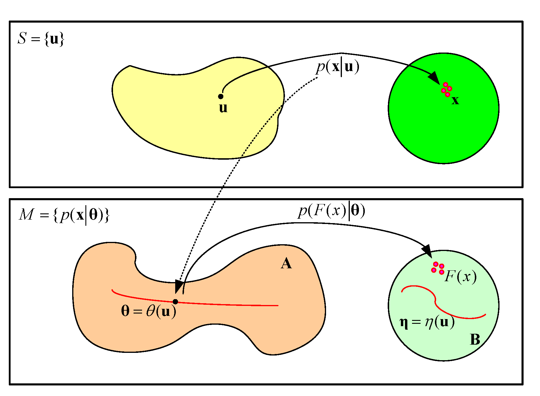
2.2. Information Geometry Probability Model

In the cooperative positioning network, the positioning information of each cooperative node is transmitted to other nodes in the cooperative position network. The positioning accuracy of cooperative networks is mainly determined by the positioning accuracy and ranging accuracy. The change in the positioning accuracy is a nonlinear variation with arbitrary jitter. The existing cooperative position fusion technology mainly adopts attenuation coefficient to modify it such that the longer the time, the smaller the attenuation coefficient. When the positioning result of the cooperative node changes, it can only slowly increase or decrease the influence of the cooperative node on the positioning accuracy of the whole cooperative positioning network. It is difficult to realize the rapid update of cooperative node positioning information, thus limiting the engineering application of cooperative positioning technology. The flat surface of the information geometry itself is a kind of surface manifold, which is more suitable and easier to implement for complete nonlinear estimation. The complete nonlinear estimation of the information geometry transformation model is shown in Figure 2.

In the standard Euclidean space, the positioning estimation of the cooperative node D can be expressed by the likelihood function $p\left(\mathbf{x}\right|\mathbf{u})$. $\mathbf{x}$ represents the positioning sampling data. $\mathbf{u}$ represents the position coordinate vector of the cooperative node D. The likelihood function $p\left(\mathbf{x}\right|\mathbf{u})$ of cooperative node D can form a statistical manifold $S=\left\{p\right(\mathbf{x}\left|\mathbf{u}\right)\}$ in Euclidean geometry, and it can be represented by parameterizations with the natural parameter $\mathbf{\theta }$ and expectation parameter $\mathbf{\eta }$. The likelihood function $p\left(\mathbf{x}\right|\mathbf{u})$ can be smoothly embedded into the Riemann geometric manifold of the exponential distribution by mapping $\mathbf{u}\to \theta \left(\mathbf{u}\right)$, that is, in the natural parameter space $\left\{\mathbf{\theta }\right\}\in \mathbf{A}$; it becomes a curve in the space, and its parameter equation is $\{\mathbf{\theta }=\theta (\mathbf{u}\left)\right\}$. The coordinate estimation problem of cooperative node D can be solved by the curve $\mathbf{\theta }=\theta \left(\right(u\left)\right)$ in the natural parameter space $\mathbf{A}$. The right graph in the lower half of Figure 2 represents the expected parameter space $\mathbf{\eta }\in \mathbf{B}$. The expected parameter space $\mathbf{B}$ and the natural parameter space $\mathbf{A}$ are dual. Dots represent the positioning information data after conversion in the expected parameter space $\mathbf{B}$, and the corresponding relationship between the natural parameter space and expected parameter space can be established by the Legendre transformation. The nonlinear likelihood function $p\left(\mathbf{x}\right|\mathbf{u})$ is transformed into a standard family of exponential distributions $p\left(\mathbf{F}\right(\mathbf{x}\left)\right|\mathbf{\theta })$ by parametric reconstruction, where $\mathbf{F}\left(\mathbf{x}\right)$ represents sufficient statistics of the positioning information data. It can obtain the coordinate estimation natural parameter value $\mathbf{\theta }$ of cooperative nodes by linear estimation of the sufficient statistics $\mathbf{F}\left(\mathbf{x}\right)$; then, mapping can be conducted from $\mathbf{\theta }$ to $\mathbf{u}$ to obtain the positioning result of the cooperative node D. Based on the theory of information geometry, the position estimation of cooperative nodes is fitted to a point on the exponential geometric manifold; among them, the nonlinear characteristics of the positioning information data are reflected in the geometric structure change of the manifold, and the nonlinear solution of the position result can make full use of the geometrical characteristics of the manifold. On the other hand, differential geometry can be applied to solve manifold problems, and a geodesic iteration instead of a state update in the Kalman filter can yield better positioning results in the cooperative network fusion positioning system.

3. Information-Geometry-Assisted Cooperative Positioning (IG-CP)

To calculate the positioning of the node D, two groups of distance differences are adopted to construct the phase interference positioning model, two nodes among A, B, C, and D are selected as transmitters, and two sinusoidal signals with a small frequency difference are transmitted to form a differential frequency interference signal [35]. The remaining two nodes act as receivers, and the distance between the four nodes can be calculated according to the phase difference of the received signal, which can be used to eliminate the positioning ambiguity of nodes. For example, if nodes A and B are assumed to be transmitters and nodes C and D are assumed to be receivers, the corresponding phase interference positioning measurements can be expressed as:

$$\begin{array}{ccc}\hfill k_{A,B,C,D}& =& \parallel {\mathbf{X}}_D-{\mathbf{X}}_A\parallel -\parallel {\mathbf{X}}_D-{\mathbf{X}}_B\parallel +\parallel {\mathbf{X}}_B-{\mathbf{X}}_C\parallel -\parallel {\mathbf{X}}_A-{\mathbf{X}}_C\parallel \hfill \end{array}$$

(1)

where ${\mathbf{X}}_A$, ${\mathbf{X}}_B$, ${\mathbf{X}}_C$, and ${\mathbf{X}}_D$ represent the position coordinates of four cooperative nodes, respectively. $\parallel {\mathbf{X}}_D-{\mathbf{X}}_A\parallel$ represents the distance between A and D; thus, Equation (1) can be rewritten as follows:

$$\begin{array}{c}\hfill k_{A,B,C,D}=d_{AD}-d_{BD}+d_{BC}-d_{AC}\end{array}$$

(2)

When positioning node D in the point wireframe of Figure 1, it is also possible to set nodes A and C as transmitters and nodes B and D as receivers, and the corresponding phase interference positioning measurement can be expressed as follows:

$$\begin{array}{c}\hfill k_{A,C,B,D}=d_{AD}-d_{CD}+d_{BC}-d_{AB}\end{array}$$

(3)

The measurement vector $k_{\left(u\right)}$ of phase interference positioning is established by using two measurement sets of the cooperative node D, which is expressed as follows:

$$\begin{array}{ccc}\hfill k_{\left(u\right)}& =& \left[\begin{array}{c}{k}_{A,B,C,D}\\ k_{A,C,B,D}\end{array}\right]\hfill \end{array}$$

(4)

$$\begin{array}{ccc}\hfill k_{A,B,C,D}& =& {\delta }_{ab}+\sqrt{{(x_a-u_x)}^2+{(y_a-u_y)}^2}-\sqrt{{(x_b-u_x)}^2+{(y_b-u_y)}^2}+d_{BC}-d_{AC}\hfill \end{array}$$

(5)

$$\begin{array}{ccc}\hfill k_{A,C,B,D}& =& {\delta }_{ac}+\sqrt{{(x_a-u_x)}^2+{(y_a-u_y)}^2}-\sqrt{{(x_c-u_x)}^2+{(y_c-u_y)}^2}+d_{BC}-d_{AB}\hfill \end{array}$$

(6)

where $\mathbf{u}={[u_x,u_y]}^T$ represents the position coordinates of the cooperative node D, which are to be estimated using unknown parameters. ${\delta }_{ab}$ and ${\delta }_{ac}$ represent the distance measurement errors. Therefore, the general phase interference positioning model of a cooperative node can be expressed as follows:

$$\begin{array}{c}\hfill \mathbf{x}=k\left(\mathbf{u}\right)+\mathbf{w}\\ \hfill \mathbf{w}\sim N(0,{\Sigma }_w)\\ \hfill {\Sigma }_w={\sigma }^2{\mathbf{I}}_{2\times 2}\end{array}$$

(7)

where $\mathbf{w}$ represents the distance measurement error vector, $\mathbf{x}$ represents the measurement data, and ${\sigma }^2$ represents the variance in $\mathbf{x}$. However, the position ambiguity error of a node is not considered in the above cooperative positioning model, which is too ideal. To fit a real cooperative positioning network, each cooperative node must be completely independent, and it is assumed that the positioning error of each cooperative node is an independent zero-mean Gaussian distribution error. Taking the cooperative nodes A, B, and C as examples, the position error is recorded as $n_a$, $n_b$, and $n_c$. After the node position error is introduced, Equation (5) can be expressed as

$$\begin{array}{ccc}\hfill k_{A,B,C,D}^{{}^{\prime }}& =& {\delta }_{ab}^{{}^{\prime }}+\sqrt{{(x_a-u_x+n_{a,x})}^2+{(y_a-u_y+n_{a,y})}^2}\hfill \\ & & -\sqrt{{(x_b-u_x+n_{b,x})}^2+{(y_b-u_y+n_{b,y})}^2}+d_{BC}-d_{AC}\hfill \end{array}$$

(8)

$$\begin{array}{ccc}\hfill {\delta }_{ab}^{{}^{\prime }}& =& \sqrt{[(x_b+n_{b,x})-(x_c+n_{c,x})]{}^2+[(y_b+n_{b,y})-(y_c+n_{c,y})]{}^2}\hfill \\ & & +\sqrt{[(x_a+n_{a,x})-(x_c+n_{c,x})]{}^2+{[(y_a+n_{a,y})-(y_c+n_{c,y})]}^2}\hfill \end{array}$$

(9)

In the process of cooperative network positioning, the errors along each axis of every cooperative node are completely independent, being set as $n_{i,x}$ and $n_{i,y}$, with i representing the cooperative node number. According to statistical theory, when the position of cooperative node A contains Gaussian noise, we utilized Rice distribution model to construct the distance measurement r between A and D, where $d=\sqrt{{(x_a-u_x)}^2+{(y_a-u_y)}^2}$ is the real distance from cooperative node A to cooperative node D. Its probability density function can be expressed as follows:

$$\begin{array}{c}\hfill f\left(r\right|d,\sigma )=\frac{r}{{\sigma }^2}exp(-\frac{r^2+d^2}{2{\sigma }^2})I_0\left(\frac{rd}{{\sigma }^2}\right)\end{array}$$

(10)

where $r=\sqrt{{(x_a-u_x+n_{a,x})}^2+{(y_a-u_y+n_{a,y})}^2}$, $\sigma$ represents the standard deviation of the measurement noise, and function $I_0\left(z\right)$ represents a zero-order modified Bessel function of the first kind:

$$\begin{array}{c}\hfill z=\frac{rd}{{\sigma }^2}\approx \frac{d^2}{{\sigma }^2}={\left[\frac{\sqrt{{(x_a-u_x)}^2+{(y_a-u_y)}^2}}{\sigma }\right]}^2\gg 1\end{array}$$

(11)

Since the distance measurement between cooperative nodes is usually more than 100 times the standard deviation of noise, the last term of Equation 10 can be approximated as follows:

$$\begin{array}{c}\hfill I_0\left(z\right)\approx \frac{e^z}{\sqrt{2\pi z}},z\gg 1\end{array}$$

(12)

Therefore, the probability density measurement function between cooperative nodes can be rewritten as:

$$\begin{array}{c}\hfill f\left(r\right|d,\sigma )\approx \frac{r}{{\sigma }^2}exp(-\frac{r^2+d^2}{2{\sigma }^2})exp\left(\frac{rd}{{\sigma }^2}\right){\left(\frac{2\pi rd}{{\sigma }^2}\right)}^{-\frac{1}{2}}=\sqrt{\frac{r}{2\pi d{\sigma }^2}}exp[-\frac{{(r-d)}^2}{2{\sigma }^2}]\end{array}$$

(13)

Furthermore, the measured distance r between cooperative nodes can be approximated by a Gaussian distribution [36] with a mean value $\mu =\sqrt{d^2+{\sigma }^2}$ and standard deviation $\sigma$, namely:

$$\begin{array}{c}\hfill r\sim N(\mu ,{\sigma }^2)\end{array}$$

(14)

When the measurement distance between cooperative nodes obeys the Gaussian distribution and is more than 100 times less than the measurement distance, Taylor series expansion can be utilized to approximate the distance. Taking the measurement distance between A and D as an example, $\eta$ and $\xi$ represent the distance measurement components on the x-axis and y-axis, respectively. The measurement distance between A and D is expressed as a function of two variables $\eta$ and $\xi$ as follows:

$$\begin{array}{c}\hfill f(\eta ,\xi )=\sqrt{{\eta }^2+{\xi }^2}\\ \hfill \eta =x_a-u_x,\xi =y_a-u_y\end{array}$$

(15)

Since the position error is included in the cooperative node A, the distance measurement can be rewritten as

$$\begin{array}{c}\hfill r=f(\eta +n_{a,x},\xi +n_{a,y})=\sqrt{{(\eta +n_{a,x})}^2+{(\xi +n_{a,y})}^2}\end{array}$$

(16)

Expanding the Taylor series of the function $f(\eta +n_{a,x},\xi +n_{a,y})$ at point $(\eta ,\xi )$ yields

$$\begin{array}{c}\hfill f(\eta +n_{a,x},\xi +n_{a,y})=f(\eta ,\xi )+n_{a,x}{\dot{f}}_{\eta }(\eta ,\xi )+n_{a,y}{\dot{f}}_{\xi }(\eta ,\xi )+\cdots \end{array}$$

(17)

$$\begin{array}{c}\hfill {\dot{f}}_{\eta }(\eta ,\xi )=\frac{\eta }{\sqrt{{\eta }^2+{\xi }^2}},{\dot{f}}_{\xi }(\eta ,\xi )=\frac{\xi }{\sqrt{{\eta }^2+{\xi }^2}}\end{array}$$

(18)

Due to the position error of cooperative node A being far less than the measurement distance, the influence of higher-order terms in the Taylor expansion is very small, and the distance between cooperative nodes A and D can be approximated as follows:

$$\begin{array}{ccc}\hfill r& =& \sqrt{{(x_a-u_x+n_{a,x})}^2+{(y_a-u_y+n_{a,y})}^2}\hfill \\ & =& \sqrt{{(x_a-u_x)}^2+{(y_a-u_y)}^2}+n_{a,x}\frac{x_a-u_x}{\sqrt{{(x_a-u_x)}^2+{(y_a-u_y)}^2}}\hfill \\ & & +n_{a,y}\frac{y_a-u_y}{\sqrt{{(x_a-u_x)}^2+{(y_a-u_y)}^2}}\hfill \end{array}$$

(19)

The position errors $n_{a,x}$ and $n_{a,y}$ comprise a Gaussian distribution with zero mean; thus, the sum of the two position errors still obeys the Gaussian distribution, and the mean ${\mu }_s$ and variance ${\sigma }_s$ are expressed as follows:

$$\begin{array}{c}\hfill {\mu }_s=0\end{array}$$

(20)

$$\begin{array}{ccc}\hfill {\sigma }_s& =& {\left(\frac{x_a-u_x}{\sqrt{{(x_a-u_x)}^2+{(y_a-u_y)}^2}}\right)}^2{\sigma }_a^2+{\left(\frac{y_a-u_y}{\sqrt{{(x_a-u_x)}^2+{(y_a-u_y)}^2}}\right)}^2{\sigma }_a^2\hfill \\ & =& {\sigma }_a\hfill \end{array}$$

(21)

where ${\sigma }_a$ represents the standard deviation of the position error of collaboration node A. The distance between cooperative nodes A and D can be approximately expressed by the following Gaussian distribution:

$$\begin{array}{c}\hfill r\sim N(\sqrt{{(x_a-u_x)}^2+{(y_a-u_y)}^2},{\sigma }_a^2)\end{array}$$

(22)

From Equation (22), it can be seen that the position error does not affect the distance measurement distribution between cooperative nodes. According to the approximate result of the Taylor-expanded distance measurement shown in Equation (17), $d_{AD}$, $d_{BD}$, $d_{BC}$, and $d_{AC}$ represent the ideal measurement distances between cooperative nodes as follows:

$$\begin{array}{ccc}\hfill d_{AD}& =& \sqrt{{(x_a-u_x)}^2+{(y_a-u_y)}^2}\hfill \\ \hfill d_{BD}& =& \sqrt{{(x_b-u_x)}^2+{(y_b-u_y)}^2}\hfill \\ \hfill d_{BC}& =& \sqrt{{(x_b-x_c)}^2+{(x_b-x_c)}^2}\hfill \\ \hfill d_{AC}& =& \sqrt{{(x_a-x_c)}^2+{(y_a-x_c)}^2}\hfill \end{array}$$

(23)

The distance measurement related to the positioning solution of cooperative node D is as follows:

$$\begin{array}{ccc}\hfill d_{AD}^{{}^{\prime }}& =& \sqrt{{(x_a-u_x+n_{a,x})}^2+{(y_a-u_y+n_{a,y})}^2}\hfill \\ & \approx & d_{AD}+\frac{x_a-u_x}{d_{AD}}{n}_{a,x}+\frac{y_a-u_y}{d_{AD}}{n}_{a,y}\hfill \end{array}$$

(24)

$$\begin{array}{ccc}\hfill d_{BD}^{{}^{\prime }}& =& \sqrt{{(x_b-u_x+n_{b,x})}^2+{(y_b-u_y+n_{b,y})}^2}\hfill \\ & \approx & d_{BD}+\frac{x_b-u_x}{d_{BD}}{n}_{b,x}+\frac{y_b-u_y}{d_{BD}}{n}_{b,y}\hfill \end{array}$$

(25)

$$\begin{array}{ccc}\hfill d_{BC}^{{}^{\prime }}& =& \sqrt{{(x_b-x_c+n_{b,x}-n_{c,x})}^2+{(y_b-y_c+n_{b,y}-n_{c,y})}^2}\hfill \\ & \approx & d_{BC}+\frac{x_b-x_c}{d_{BC}}(n_{b,x}-n_{c,x})+\frac{y_b-y_c}{d_{BC}}(n_{b,y}-n_{c,y})\hfill \end{array}$$

(26)

$$\begin{array}{ccc}\hfill d_{AC}^{{}^{\prime }}& =& \sqrt{{(x_a-x_c+n_{a,x}-n_{c,x})}^2+{(y_a-y_c+n_{a,y}-n_{c,y})}^2}\hfill \\ & \approx & d_{AC}+\frac{x_a-x_c}{d_{AC}}(n_{a,x}-n_{c,x})+\frac{y_a-y_c}{d_{AC}}(n_{a,y}-n_{c,y})\hfill \end{array}$$

(27)

The phase interference positioning measurement with position error $k_{A,B,C,D}^{{}^{\prime }}$ can be expressed as

$$\begin{array}{ccc}\hfill k_{A,B,C,D}^{{}^{\prime }}& \approx & (\frac{x_a-u_x}{d_{AD}}-\frac{x_a-x_c}{d_{AC}})n_{a,x}+(\frac{x_a-u_x}{d_{AD}}-\frac{x_a-x_c}{d_{AC}})n_{a,y}+(\frac{x_b-x_c}{d_{BC}}-\frac{x_b-u_x}{d_{BD}})n_{b,x}\hfill \\ & & +(\frac{y_b-y_c}{d_{BC}}-\frac{y_b-u_y}{d_{BD}})n_{b,y}+(\frac{x_a-x_c}{d_{AC}}-\frac{x_b-x_c}{d_{BC}})n_{c,x}+(\frac{y_a-y_c}{d_{AC}}-\frac{y_b-y_c}{d_{BC}})n_{c,y}\hfill \end{array}$$

(28)

Because the position errors of cooperative nodes along each axis are completely independent, the variance ${\sigma }_{s1}^2$ in the sum of the six position error terms in (28) can be obtained as follows:

$$\begin{array}{ccc}\hfill {\sigma }_{s1}^2& =& 2[1-\frac{(x_a-u_x)(x_a-x_c)+(y_a-u_y)(y_a-y_c)}{d_{AD}{d}_{AC}}]{\sigma }_a^2\hfill \\ & & +2[1-\frac{(x_b-u_x)(x_b-x_c)+(y_b-u_y)(y_b-y_c)}{d_{BD}{d}_{BC}}]{\sigma }_b^2\hfill \\ & & +2[1-\frac{(x_a-x_c)(x_b-x_c)+(y_a-y_c)(y_b-y_c)}{d_{AC}{d}_{BC}}]{\sigma }_c^2\hfill \end{array}$$

(29)

Similarly, the variance ${\sigma }_{s2}^2$ in another measurement $k_{A,C,B,D}^{{}^{\prime }}$ is as follows:

$$\begin{array}{ccc}\hfill {\sigma }_{s2}^2& =& 2[1-\frac{(x_a-u_x)(x_a-x_b)+(y_a-u_y)(y_a-y_b)}{d_{AD}{d}_{AB}}]{\sigma }_a^2\hfill \\ & & +2[1-\frac{(x_a-x_b)(x_c-x_b)+(y_a-y_b)(y_c-y_b)}{d_{AB}{d}_{BC}}]{\sigma }_b^2\hfill \\ & & +2[1-\frac{(x_c-u_x)(x_c-x_b)+(y_c-u_y)(y_c-y_b)}{d_{BC}{d}_{CD}}]{\sigma }_c^2\hfill \end{array}$$

(30)

When the cooperative nodes have positioning errors, the phase interference positioning distance measurement values $k_{A,B,C,D}^{{}^{\prime }}$ and $k_{A,C,B,D}^{{}^{\prime }}$ have approximately the following distributions.

$$\begin{array}{ccc}\hfill k_{A,B,C,D}^{{}^{\prime }}& \sim & N(k_{A,B,C,D},{\sigma }_{s1}^2)\hfill \\ \hfill k_{A,C,B,D}^{{}^{\prime }}& \sim & N(k_{A,C,B,D},{\sigma }_{s2}^2)\hfill \end{array}$$

(31)

In a real situation where the cooperative node has a position error, the general phase interference positioning model of the cooperative node can be expressed as follows:

$$\begin{array}{c}\hfill \mathbf{x}=k\left(\mathbf{u}\right)+n\left(\mathbf{u}\right)+k\left(\mathbf{w}\right)\end{array}$$

(32)

$n\left(\mathbf{u}\right)$ represents the equivalent distribution of cooperative positioning node position errors, which is fitted to a Gaussian distribution with a mean value of 0 and variance of ${\Sigma }_s=diag({\sigma }_{s1}^2,{\sigma }_{s2}^2)$ in our model. $\mathbf{w}$ represents the measurement error of the phase interference positioning distance. Due to the measurement of the distance being completely independent in the phase interference positioning, $\mathbf{x}$ represents the positioning sampling data, $\mathbf{u}$ represents the position coordinate vector of the cooperative node, ${\Sigma }_w$ represents the variance of noise, and ${\Sigma }_s$ represents the variance of position coordinate vector. T he conditional probability distribution between the measurement value and the optimal estimation value is as follows.

$$\begin{array}{c}\hfill \mathbf{x}|\mathbf{u}\sim N(\mu \left(\mathbf{u}\right),\Sigma \left(\mathbf{u}\right))\\ \hfill \mu \left(\mathbf{u}\right)=k\left(\mathbf{u}\right),\Sigma \left(\mathbf{u}\right)={\Sigma }_s+{\Sigma }_w\end{array}$$

(33)

The natural gradient method based on the statistical manifold is adopted to realize optimal positioning coordinate estimation of the cooperative node D, and according to the phase interference positioning measurement distribution given in Equation (33), the likelihood function of the measured value can be expressed as follows:

$$\begin{array}{c}\hfill p\left(\mathbf{x}\right|\mathbf{u})=|2\pi {\Sigma }_w|{}^{-\frac{1}{2}}exp(-\frac{1}{2}{(\mathbf{x}-k\left(\mathbf{u}\right))}^T{\Sigma }_w^{-1}(\mathbf{x}-k\left(\mathbf{u}\right)))\end{array}$$

(34)

The Gaussian probability density function shown in Equation (34) can be arranged into a standard bending index distribution form:

$$\begin{array}{ccc}\hfill p\left(\mathbf{x}\right|\mathbf{u})& \approx & exp(C\left(\mathbf{x}\right)+{\mathbf{\theta }}^T\left(\mathbf{u}\right)\mathbf{F}\left(\mathbf{x}\right)-\phi \left(\mathbf{\theta }\left(\mathbf{u}\right)\right))\hfill \\ & =& p\left(\mathbf{x}\right|\mathbf{\theta }\left(\mathbf{u}\right))\hfill \end{array}$$

(35)

According to Equation (35), in information geometry, it is necessary to establish a new parametric representation of natural parameters on the geometric manifold, where the natural parameters of the cooperative positioning nodes are set to $(\mathbf{\theta },\mathsf{\Theta })$. The relationship between the natural parameter and the local parameter u is as follows:

$$\left[\begin{array}{c}\mathbf{\theta }\\ \mathsf{\Theta }\end{array}\right]=\left[\begin{array}{c}{\Sigma }^{-1}\left(\mathbf{u}\right)\mu \left(\mathbf{u}\right)\\ -\frac{1}{2}{\Sigma }^{-1}\left(\mathbf{u}\right)\end{array}\right]$$

(36)

To simplify the calculation, the sufficient statistics of the Gaussian distribution of the measured value are set as a linear model

$$\begin{array}{c}\hfill F\left(\mathbf{x}\right)=\mathbf{x}\end{array}$$

(37)

On the geometric manifold, the potential function distributed $\phi (\mathbf{\theta },\mathsf{\Theta })$ can be expressed by local parameters as follows:

$$\begin{array}{c}\hfill \phi (\mathbf{\theta },\mathsf{\Theta })=\frac{1}{2}{\mu }^T{\Sigma }^{-1}\mu +\frac{1}{2}log|\Sigma |+\frac{n}{2}log2\pi \end{array}$$

(38)

where n represents the dimension of $\mu \left(\mathbf{u}\right)$ or the potential of a set. The maximum-likelihood estimation $\widehat{\mathbf{u}}$ of the local parameter $\mathbf{u}$ can be obtained by solving the following maximum-likelihood equation:

$$\begin{array}{ccc}\hfill \nabla l\left(\widehat{\mathbf{u}}\right)& =& \nabla lnp\left(\mathbf{x}\right|\mathbf{u})\hfill \\ & =& \nabla {\mathbf{\theta }}^T\left(\widehat{\mathbf{u}}\right)[F\left(\mathbf{x}\right)-\eta \left(\widehat{\mathbf{u}}\right)]=0\hfill \end{array}$$

(39)

where $l\left(\widehat{\mathbf{u}}\right)$ represents the logarithmic likelihood function and $\eta$ represents the expectation function. According to the properties of the bending index distribution, the expected parameter $\mathbf{\eta }$ and the Fisher information matrix $G\left(\mathbf{\theta }\right)$ of the natural parameter can be obtained from the derivative of $\mathbf{\theta }$ by the potential function $\phi \left(\mathbf{\theta }\right)$ as follows:

$$\begin{array}{c}\hfill \eta \left(\mathbf{u}\right)={\nabla }_{\theta }\phi \left(\mathbf{\theta }\right)=-\frac{1}{2}{\mathsf{\Theta }}^{-1}\mathbf{\theta }=k\left(\mathbf{u}\right)\end{array}$$

(40)

$$\begin{array}{c}\hfill G\left(\mathbf{\theta }\right)={\nabla }_{\theta }{\nabla }_{\theta }^T\phi \left(\mathbf{\theta }\right)=-\frac{1}{2}{\mathsf{\Theta }}^{-1}={\Sigma }_w\end{array}$$

(41)

The Jacobian matrix of the natural parameter $\mathbf{\theta }$ with respect to the local parameter $\mathbf{u}$ of the cooperative node positioning coordinate is expressed as:

$$\begin{array}{ccc}\hfill \nabla \theta \left(\mathbf{u}\right)& =& {\Sigma }_w^{-1}{\nabla }_{u}k\left(\mathbf{u}\right)\hfill \\ & =& {\Sigma }_w^{-1}\left[\begin{array}{cc}\frac{\partial k_{A,B,C,D}}{\partial u_x}& \frac{\partial k_{A,B,C,D}}{\partial u_y}\\ \frac{\partial k_{A,C,B,D}}{\partial u_x}& \frac{\partial k_{A,C,B,D}}{\partial u_y}\end{array}\right]\hfill \end{array}$$

(42)

where

$$\begin{array}{ccc}\hfill \frac{\partial k_{A,B,C,D}}{\partial u_x}& =& \frac{x_b-u_x}{\sqrt{(x_b-u_x){}^2+(y_b-u_y){}^2}}-\frac{x_a-u_x}{\sqrt{{(x_a-u_x)}^2+{(y_a-u_y)}^2}}\hfill \\ \hfill \frac{\partial k_{A,B,C,D}}{\partial u_x}& =& \frac{x_b-u_x}{\sqrt{(x_b-u_x){}^2+(y_b-u_y){}^2}}-\frac{x_a-u_x}{\sqrt{{(x_a-u_x)}^2+{(y_a-u_y)}^2}}\hfill \\ \hfill \frac{\partial k_{A,B,C,D}}{\partial u_x}& =& \frac{x_b-u_x}{\sqrt{(x_b-u_x){}^2+(y_b-u_y){}^2}}-\frac{x_a-u_x}{\sqrt{{(x_a-u_x)}^2+{(y_a-u_y)}^2}}\hfill \\ \hfill \frac{\partial k_{A,B,C,D}}{\partial u_x}& =& \frac{x_b-u_x}{\sqrt{(x_b-u_x){}^2+(y_b-u_y){}^2}}-\frac{x_a-u_x}{\sqrt{{(x_a-u_x)}^2+{(y_a-u_y)}^2}}\hfill \end{array}$$

(43)

The Fisher information matrix of the local parameter $\mathbf{u}$ is

$$\begin{array}{ccc}\hfill G\left(\mathbf{u}\right)& =& \nabla {\mathbf{\theta }}^T\left(\mathbf{u}\right)G\left(\mathbf{\theta }\right)\nabla \theta \left(\mathbf{u}\right)\hfill \\ & =& {\nabla }_u^{T}k\left(\mathbf{u}\right){\Sigma }_w^{-1}{\nabla }_{u}k\left(\mathbf{u}\right)\hfill \end{array}$$

(44)

On the geometric manifold of natural parameters, maximum-likelihood parameter estimation of the bending exponential distribution family is adopted to obtain the positioning of the cooperative node D, and estimation update of the positioning coordinate $\mathbf{u}$ is as follows:

$$\begin{array}{ccc}\hfill {\mathbf{u}}^{k+1}& =& {\mathbf{u}}^k+\lambda G^{-1}\left({\mathbf{u}}^k\right)\nabla l\left({\mathbf{u}}^k\right)\hfill \\ & =& {\mathbf{u}}^k+\lambda G^{-1}\left({\mathbf{u}}^k\right)\nabla {\theta }^T\left({\mathbf{u}}^k\right)(F\left(\mathbf{x}\right)-\eta \left({\mathbf{u}}^k\right))\hfill \end{array}$$

(45)

where $\lambda$ represents the iterative step size. When the new local parameter ${\mathbf{u}}^{k+1}$ of the positioning coordinate is obtained, the Fisher information matrix $G\left(\mathbf{u}\right)$ of the information geometric plane needs to be updated, as shown below:

$$\begin{array}{c}\hfill G\left({\mathbf{u}}^{k+1}\right)={\left({\nabla }_{u}k\left({\mathbf{u}}^{k+1}\right)\right)}^T{\Sigma }_w^{-1}{\nabla }_{u}k\left({\mathbf{u}}^{k+1}\right)\end{array}$$

(46)

We utilized the iterative calculation method proposed in reference [29]: when the difference value $e^{k+1}$ between two iterations is less than a certain threshold $th$, the iteration terminates, which is expressed as follows:

$$\begin{array}{c}\hfill e^{k+1}=\parallel {\mathbf{u}}^k-{\mathbf{u}}^{k+1}\parallel <th\end{array}$$

(47)

The estimated value ${\mathbf{u}}^{k+1}$ is considered as the actual coordinate of the collaboration node. The flow of our IG-CP algorithm is shown in Figure 3.

The natural gradient utilizes the local curvature of the geometric manifold to modify the iterative direction of the standard gradient, which can result in a faster convergence rate. In addition, the Fisher information matrix is updated at the same time in each iteration based on the natural gradient estimation, which can meet the real-time fitting of the nonlinear positioning error and ranging error of the cooperative positioning system. It can effectively improve the accuracy and stability of cooperative positioning.

4. Simulation Results and Analysis

4.1. Ideal Condition Simulation

The size of the cooperative positioning network is 1000 m × 1000 m. In the cooperative network, the coordinates of the known cooperative nodes are (200 m, 200 m), (800 m, 100 m), and (500 m, 900 m), and the variance of the positioning errors of nodes with known positions is 1 m. The true coordinates of the unknown position node are at (500 m, 500 m), and the variance of the positioning error of an unknown node is 5 m. The measurement distance between cooperative nodes is the real value, and the ranging error is 0 m. On the plane of the geometric manifold with natural parameters, the probability density distribution of locating nodes is fused, and the maximum estimation of the probability density distribution is considered as the positioning result of the unknown cooperative node. The simulation results are shown in Figure 4.

From Figure 4, we can see that the ranging error is 0 under the ideal condition of cooperative positioning. After the iterative convergence is completed, the optimal position estimation value of the cooperative node with an unknown position is exactly the same as the real position value, both of which are (500 m, 500 m), and the distribution probability density of the position is the same as that of the cooperative node at the unknown position. This result shows that the IG-CP algorithm, which utilizes the information probability to achieve cooperative positioning, can reduce the positioning error of cooperative nodes.

4.2. Simulation under Different Ranging Errors

In the cooperative positioning network, the ranging error will have a great impact on the positioning accuracy of the cooperative node. Existing ranging technologies mainly include radio ranging, UWB ranging, laser ranging, radar ranging, and other methods, with accuracies ranging from the cm level to the 10 m level. Therefore, the variance values of the ranging error are 10 m, 5 m, and 1 m in the simulation, and the variance of the positioning error of the cooperative node is 1 m. The distribution of the cooperative positioning network is the same as that under the ideal condition, and the simulation results are shown in Figure 5, Figure 6 and Figure 7.

From Figure 5, we can see that when the variance of the ranging error is 10 m, the unknown positioning node’s maximum probability density of the positioning error is only 0.7, far less than that of the other known positioning cooperative nodes; however, the optimal position coordinate estimation of the unknown cooperative node is the same as that in a real situation, and it is still (500 m, 500 m). The simulation results show that the proposed cooperative positioning algorithm based on information geometry can reduce the influence of the ranging error by fusing the information probability of the cooperative node in the geometric manifold. It can be seen from Figure 6 and Figure 7 that as the variance of the ranging error decreases, the maximum value of the positioning error probability density of a cooperative node with an unknown position is close to the ideal situation, and the optimal value of the positioning coordinate is kept at (500 m, 500 m). Moreover, the distribution range of the positioning error probability function also approaches the ideal situation. This outcome shows that our IG-CP algorithm can effectively reduce the influence of ranging errors between cooperative nodes. When the ranging error between nodes becomes larger, it can also ensure the stability of the positioning accuracy of the whole cooperative network.

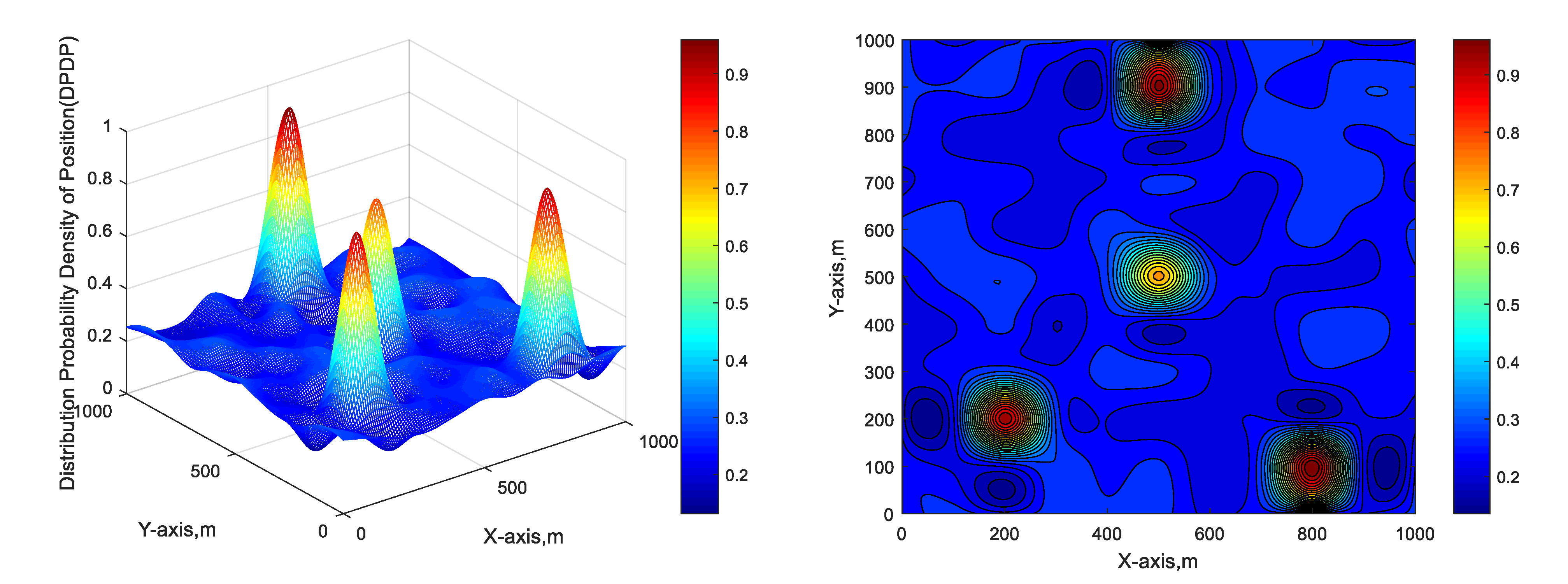
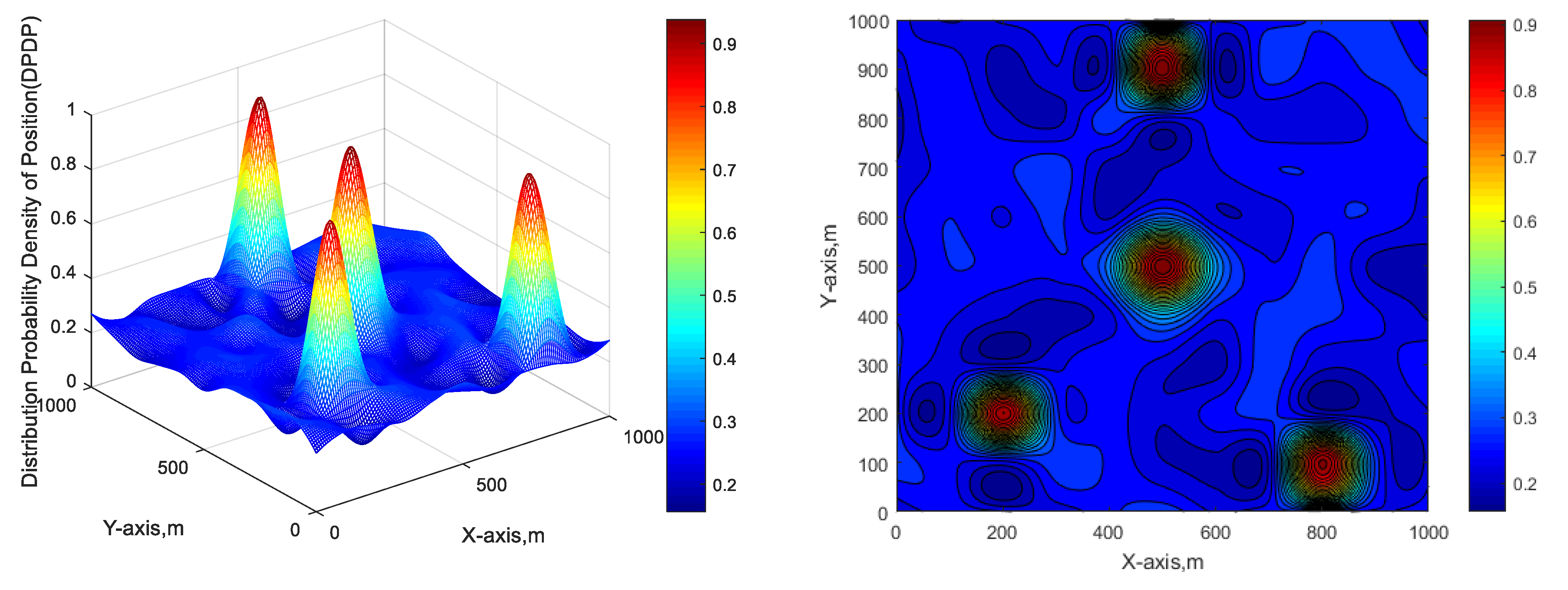
4.3. Simulation of Cooperative Positioning under Extreme Distribution

In the application of the cooperative positioning network, there will be an extreme distribution of other cooperative nodes around some edge nodes in one direction, resulting in a significant decline in the positioning accuracy of edge nodes. To verify the positioning performance in this case, the size of the cooperative positioning network is set as 1000 m × 1000 m, where the position coordinates of the known nodes are (100 m, 100 m), (100 m, 400 m), and (500 m, 200 m). The variance of the positioning error of nodes with a known position is 1 m, the real value of the position coordinate of the node with an unknown position is (800 m, 800 m), and the variance of the positioning error of the unknown node is 5 m. The variance of the ranging error between cooperative nodes is 1 m. The simulation results are shown in Figure 8.

It can be seen from Figure 8 that in the extreme distribution situation of a cooperative positioning network, the optimal positioning coordinate estimation value of edge nodes with unknown positions is still approximately (800 m, 800 m), but the maximum probability density is approximately 0.7, which can ensure the positioning accuracy of edge nodes. This result shows that the positioning of edge nodes is very difficult. All positioning error probability functions fused on an information geometric manifold can reduce the accumulation of error in one direction. This process can effectively reduce the impact of the extreme distribution of a cooperative position network and realize highly accurate cooperative positioning under any topology distribution.

4.4. Integrated Positioning Simulation under a Multinode Network

In the development of the cooperative positioning network, the number of nodes increases exponentially. Because of the cost and load, most of the nodes have only one or no navigation source; thus, it is necessary to improve the accuracy by cooperative positioning. In this section, the scope of the cooperative positioning network is also set to 1000 m × 1000 m, and the total number of cooperative nodes is 20. Among them, the variance of the positioning error of any five nodes is 1 m, and that of the other nodes is 5 m. The variance of the ranging error between cooperative nodes is 1 m. The simulation result is shown in Figure 9.

After multiple iterations, the optimal positioning estimates of all cooperative nodes are close to the real positions. According to the positioning error probability density distribution of cooperative nodes, the positioning accuracies of all cooperative nodes are basically the same, and the maximum probability density is close to 0.9. The positioning accuracy of all cooperative nodes is similar to that of the optimal cooperative nodes. It is proved that our proposed position error probability function fusion technology can quickly realize the positioning of the whole cooperative positioning network, eliminate the influence of the ranging error, and improve the positioning accuracy of the whole cooperative network.

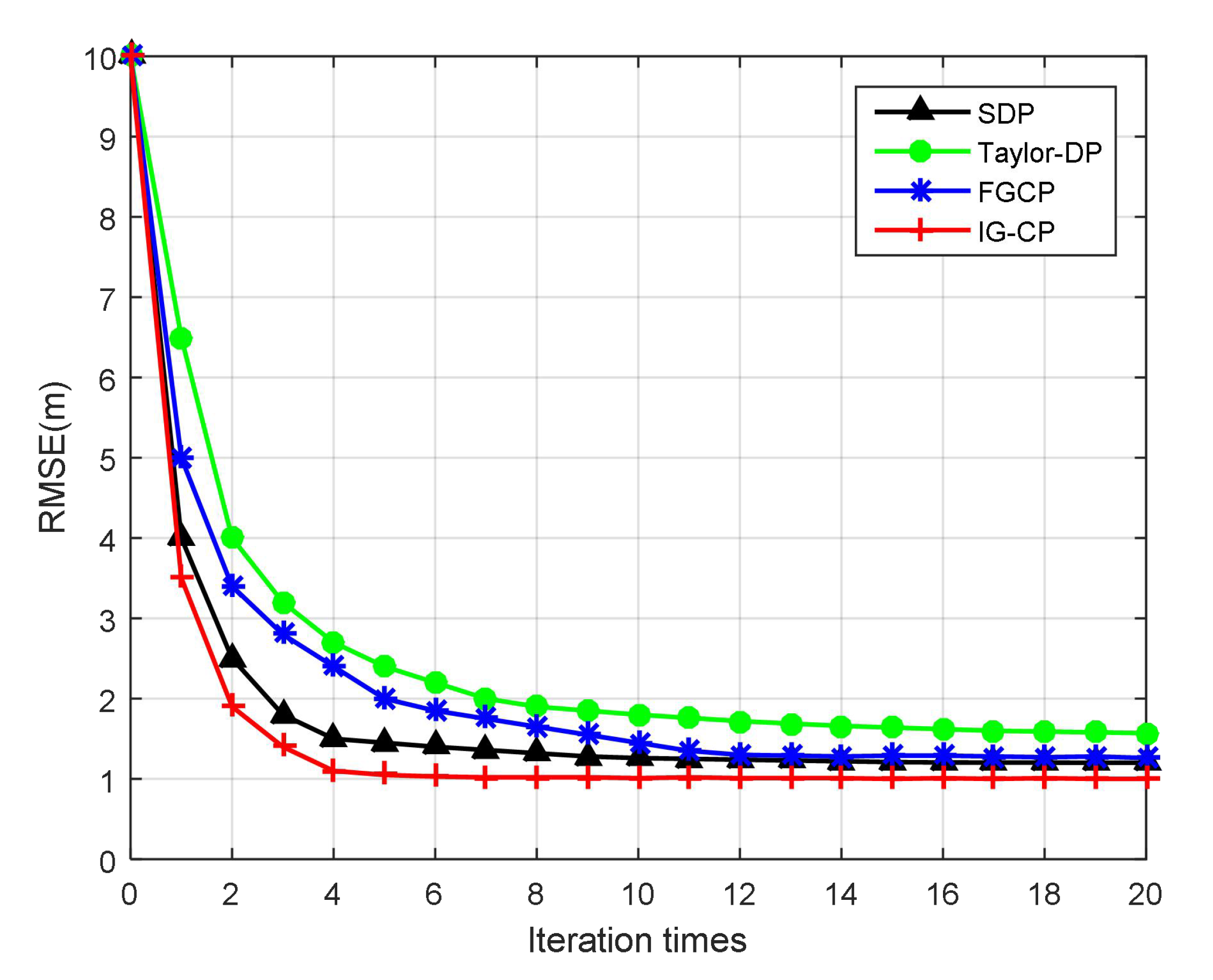
4.5. Simulation Analysis of the Convergence Rate

In the cooperative positioning network, the convergence rate is an extremely important index, as it is the key factor of the application of the cooperative positioning network. Among them, the variance of the positioning error of any five nodes is 1 m, that of other nodes is 6 m, and the variance of the ranging error between cooperative nodes is 3 m, after T = 100 Monte Carlo simulations. To compare with the performance of the existing cooperative positioning algorithm, the IG-CP algorithm proposed in this paper is compared with the SDP algorithm proposed in [6], the Taylor-DP algorithm proposed in [8], and the FGCP proposed in [9]. The simulation results are shown in Figure 10.

In Figure 10, the positioning errors of the four algorithms decrease and tend to converge with the increase in the number of iterations. The Taylor–DP algorithm requires 15 iterations to complete the convergence, and the MMSE is 1.7 m. The convergence rate of the FGCP algorithm is better than that of the Taylor–DP algorithm. The FGCP needs 12 iterations to complete the convergence, while the MMSE requires approximately 1.3 m. The convergence rate of the SDP is lower than that of our IG-CP algorithm and better than that of the other algorithm, and it requires eight iterations to complete the iterative convergence. The MMSE is close to the FGCP algorithm, requiring approximately 1.3 m. Our IG-CP algorithm has the fastest convergence speed, with convergence being completed in approximately five iterations. The MMSE of IG-CP is close to 1 m, which is equivalent to the cooperative node with the highest positioning accuracy.

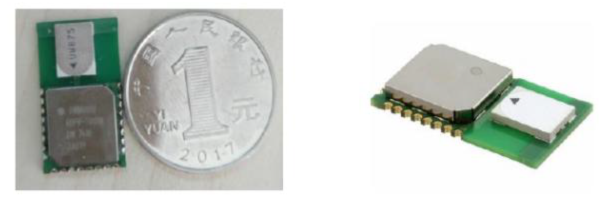
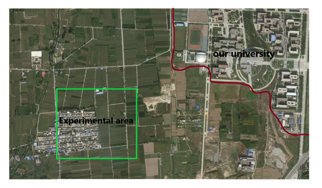
4.6. Real-Environment Test

The IG-CP algorithm was tested in a real environment by using sensor nodes to construct a cooperative positioning network. The DWM1000 module is adopted to construct the cooperative node, and the distance between the cooperative nodes is measured by the UWB communication of DWM1000 [37]. The range of the DWM1000 module is 3 km, and the measurement accuracy of the module is 0.1 m, roughly the size of a coin. The appearance is shown in Figure 11. To realize the positioning of the cooperative nodes, the STM32 development board designed by our team is utilized in the cooperative positioning system, as shown in Figure 12.

To show the positioning performance of a large-scale cooperative node network, the experimental area was a farm near our university. The area included a small village and farmland, as shown in Figure 13. Twenty cooperative nodes were randomly set in the range of 1000 m × 1000 m.

The initial positioning error and ranging error depend on the node device. The simulation result is shown in Figure 14.

As can be seen in Figure 14, when the iteration is complete, the maximum probability density is close to 0.85. The positioning accuracy of all cooperative nodes is similar to that of the optimal cooperative nodes with high accuracy in the cooperative network. the optimal positioning estimates of all cooperative nodes are close to the real positions. The experimental results are in agreement with the simulation results, and the village buildings have little influence on the positioning accuracy. A few cooperative nodes are at the edge of the cooperative location network and have large fluctuation due to the influence of the accumulation of ranging errors in the same direction. However, most of the cooperative nodes can improve the positioning accuracy through the IG-CP algorithm proposed in this paper. In the real-experiment test, the algorithm processing module is implemented by the STM32 development board and can realize a real-time response, which proves that the IG-CP algorithm has low computational complexity.

5. Conclusions

The existing distributed cooperative positioning methods generally suffer from high computational complexity and a slow convergence speed; thus, it is very difficult to apply the cooperative positioning technology in practice. The probability density model of positioning error information is established using the navigation information of each cooperative node in a distributed cooperative network; then, the positioning information fusion is carried out by combining the ranging information between cooperative nodes on the plane of the geometric manifold. In this paper, a simulation analysis is carried out in terms of the ranging error, node distribution, convergence speed, and communication overhead. The simulation results show that IG-CP can reduce the influence of the ranging error on the cooperative positioning node when the magnitude of the ranging error is the same as that of the positioning error of the cooperative node. Regarding the extreme distribution of a cooperative location network, the fusion of the location information probability model can avoid the accumulation of single-direction positioning errors and improve the positioning accuracy of cooperative location nodes at the edge. In the context of iterative computation, the iterative speed of IG-CP is more than $30\%$ higher than that of the existing cooperative positioning algorithms, and the communication cost is lower than that of the other cooperative positioning algorithms. Our proposed IG-CP algorithm has lower computational complexity and a higher precision of cooperative positioning, which breaks through the shackles of existing cooperative positioning technology only from the perspective of location information fusion. It has better application value in the next generation of information technology, such as integrated space-based and ground-based networks, smart cities, driverless transport, and material distribution.

References

1. Lal, N.; Kumar, S.; Chaurasiya, V.K. A Road Monitoring Approach with Real-Time Capturing of Events for Efficient Vehicles Safety in Smart City. Wirel. Pers. Commun. 2020, 114, 657–674. [Google Scholar] [CrossRef]
2. Sultanuddin, S.J.; Ali Hussain, M. Token system-based efficient route optimization in mobile ad hoc network for vehicular ad hoc network in smart city. Trans. Emerg. Telecommun. Technol. 2020, 31, e3853. [Google Scholar] [CrossRef]
3. Aujla, G.S.; Singh, M.; Bose, A.; Kumar, N.; Han, G.; Buyya, R. BlockSDN: Blockchain-as-a-Service for Software Defined Networking in Smart City Applications. IEEE Netw. 2020, 34, 83–91. [Google Scholar] [CrossRef]
4. Neil, J.; Cosart, L.; Zampetti, G. Precise Timing for Vehicle Navigation in the Smart City: An Overview. IEEE Commun. Mag. 2020, 58, 54–59. [Google Scholar] [CrossRef]
5. Gao, Z.; Ge, M.; Li, Y.; Shen, W.; Zhang, H.; Schuh, H. Railway Irregularity Measuring Using Rauch–Tung–Striebel Smoothed Multi-sensors Fusion System: Quad-GNSS PPP, IMU, Odometer, and Track Gauge. Gps Solut. 2018, 22, 36–53. [Google Scholar] [CrossRef]
6. Paziewski, J.D.; Sieradzki, R.; Baryla, R. Multi-GNSS high-rate RTK, PPP and novel direct phase observation processing method: Application to precise dynamic displacement detection. Meas. Sci. Technol. 2018, 29, 035002. [Google Scholar] [CrossRef]
7. Szot, T.; Specht, C.; Specht, M.; Dabrowski, P.S. Comparative Analysis of Positioning Accuracy of Samsung Galaxy Smartphones in Stationary Measurements. PLoS ONE 2019, 14, e0215562. [Google Scholar] [CrossRef]
8. Zhu, M.; Wen, Y.Q. Design and Analysis of Collaborative Unmanned Surface-Aerial Vehicle Cruise Systems. J. Adv. Transp. 2019, 2019, 107–116. [Google Scholar] [CrossRef]
9. Umemoto, K.; Endo, T.; Matsuno, F. Dynamic Cooperative Transportation Control Using Friction Forces of n Multi-Rotor Unmanned Aerial Vehicles. J. Intell. Robot. Syst. 2020, 100, 1085–1095. [Google Scholar] [CrossRef]
10. Han, J.; Cho, Y.; Kim, J. Coastal SLAM with Marine Radar for USV Operation in GPS-Restricted Situations. IEEE J. Ocean. Eng. 2019, 44, 300–309. [Google Scholar] [CrossRef]
11. Xiong, J.; Cheong, J.W.; Xiong, Z.; Dempster, A.G.; List, M.; Wöske, F.; Rievers, B. Carrier-Phase-Based Multi-Vehicle Cooperative Positioning Using V2V Sensors. IEEE Trans. Veh. Technol. 2020, 69, 9528–9541. [Google Scholar] [CrossRef]
12. Kim, H.; Granström, K.; Gao, L.; Battistelli, G.; Kim, S.; Wymeersch, H. 5G mmWave Cooperative Positioning and Mapping Using Multi-Model PHD Filter and Map Fusion. IEEE Trans. Veh. Technol. 2020, 19, 3782–3795. [Google Scholar] [CrossRef] [Green Version]
13. Liu, T.; Li, G.; Lu, L.; Li, S.; Tian, S. Robust Hybrid Cooperative Positioning Via a Modified Distributed Projection-Based Method. IEEE Trans. Veh. Technol. 2020, 19, 3003–3018. [Google Scholar] [CrossRef]
14. Hamie, J.; Denis, B.; Richard, C. Decentralized Positioning Algorithm for Relative Nodes Localization in Wireless Body Area Networks. Mob. Netw. Appl. 2014, 19, 1–9. [Google Scholar] [CrossRef]
15. Zinas, N.; Parkins, A.; Ziebart, M. Improved network-based single-epoch ambiguity resolution using centralized GNSS network processing. Gps Solut. 2013, 17, 17–27. [Google Scholar] [CrossRef]
16. Yeoman, J.; Duckham, M. International Journal of Geographical Information Science. Int. J. Geogr. Inf. Sci. 2016, 30, 993–1011. [Google Scholar] [CrossRef]
17. Ayala-Garcia, D.; Curtis, A.; Branicki, M. Seismic Interferometry from Correlated Noise Sources. Remote Sens. 2021, 13, 2703. [Google Scholar] [CrossRef]
18. Mathar, R.; Schmeink, M. Optimal Base Station Positioning and Channel Assignment for 3G Mobile Networks by Integer Programming. Ann. Oper. Res. 2001, 107, 225–236. [Google Scholar] [CrossRef]
19. Raulefs, R.; Zhang, S.; Mensing, C. Bound-based spectrum allocation for cooperative positioning. Eur. Trans. Telecommun. 2013, 24, 69–83. [Google Scholar] [CrossRef] [Green Version]
20. Fathi-Kazerooni, S.; Kaymak, Y.; Rojas-Cessa, R.; Feng, J.; Ansari, N.; Zhou, M.; Zhang, T. Optimal Positioning of Ground Base Stations in Free-Space Optical Communications for High-Speed Trains. IEEE Trans. Intell. Transp. Syst. 2017, 19, 1940–1949. [Google Scholar] [CrossRef]
21. Lv, X.W.; Liu, K.H.; Hu, P. Efficient solution of additional base stations in time-of-arrival positioning systems. Electron. Lett. 2010, 46, 861–863. [Google Scholar] [CrossRef]
22. Hossain, M.A.; Elshafiey, I.; Al-Sanie, A. Cooperative vehicle positioning with multi-sensor data fusion and vehicular communications. Wirel. Netw. 2018, 25, 1403–1413. [Google Scholar] [CrossRef]
23. Ghari, P.M.; Shahbazian, R.; Ghorashi, S.A. Maximum Entropy-Based Semi-Definite Programming for Wireless Sensor Network Localization. IEEE Internet Things J. 2019, 6, 3480–3491. [Google Scholar] [CrossRef]
24. Wang, X.; Li, X.; Zhang, L.H.; Li, R.C. An Efficient Numerical Method for the Symmetric Positive Definite Second-Order Cone Linear Complementarity Problem. J. Sci. Comput. 2019, 79, 1608–1629. [Google Scholar] [CrossRef]
25. Huang, B.; Yao, Z.; Cui, X.; Lu, M. Dilution of Precision Analysis for GNSS Collaborative Positioning. IEEE Trans. Veh. Technol. 2016, 65, 3401–3415. [Google Scholar] [CrossRef]
26. Jing, H.; Pinchin, J.; Hill, C.; Moore, T. An Adaptive Weighting based on Modified DOP for Collaborative Indoor Positioning. J. Navig. 2015, 69, 1–21. [Google Scholar] [CrossRef]
27. Rife, J. Collaborative Vision-Integrated Pseudorange Error Removal: Team-Estimated Differential GNSS Corrections with no Stationary Reference Receiver. IEEE Trans. Intell. Transp. Syst. 2012, 13, 15–24. [Google Scholar] [CrossRef]
28. Cichon, D.; Psiuk, R.; Brauer, H.; Töpfer, H. A Hall-Sensor-Based Localization Method With Six Degrees of Freedom Using Unscented Kalman Filter. IEEE Sens. J. 2019, 19, 2509–2516. [Google Scholar] [CrossRef]
29. Tang, C.; Zhang, L.; Zhang, Y.; Song, H. Factor Graph-Assisted Distributed Cooperative Positioning Algorithm in the GNSS System. Sensors 2018, 18, 3748. [Google Scholar] [CrossRef] [Green Version]
30. Qi, F.; Liang, F.; Liu, M.; Lv, H.; Wang, P.; Xue, H.; Wang, J. Position-Information-Indexed Classifier for Improved Through-Wall Detection and Classification of Human Activities Using UWB Bio-Radar. IEEE Antennas Wirel. Propag. Lett. 2019, 18, 437–441. [Google Scholar] [CrossRef]
31. Jia, T.; Ho, K.C.; Wang, H.; Shen, X. Effect of Sensor Motion on Time Delay and Doppler Shift Localization: Analysis and Solution. IEEE Trans. Signal Process. 2019, 67, 5881–5899. [Google Scholar] [CrossRef]
32. Song, Z.; Zhang, Y.; Lv, H.; Chen, P.; Tang, C. Electromagnetic situation generation algorithm based on information geometry. Telecommun. Syst. 2021, 77, 171–187. [Google Scholar] [CrossRef]
33. Pereyra, M.; Batatia, H.; McLaughlin, S. Exploiting information geometry to improve the convergence of nonparametric active contours. In Proceedings of the 2013 5th IEEE International Workshop on Computational Advances in Multi-Sensor Adaptive Processing (CAMSAP), St. Martin, France, 15–18 December 2013; Volume 7, pp. 700–707. [Google Scholar]
34. Garcia, D.C.; Fonseca, T.A.; Ferreira, R.U.; de Queiroz, R.L. Geometry Coding for Dynamic Voxelized Point Clouds Using Octrees and Multiple Contexts. IEEE Trans. Image Process. 2019, 29, 313–322. [Google Scholar] [CrossRef]
35. Yang, T.; Jiang, Z.; Sun, R.; Cheng, N.; Feng, H. Maritime Search and Rescue Based on Group Mobile Computing for UAVs and USVs. IEEE Trans. Ind. Inform. 2020, 16, 7700–7708. [Google Scholar] [CrossRef]
36. Brown, L.; Steinerberger, S. On the Wasserstein distance between classical sequences and the Lebesgue measure. Trans. Am. Math. Soc. 2020, 373, 8943–8962. [Google Scholar] [CrossRef]
37. Yu, Z.; Mo, H.; Zhang, J.; Ma, Y.; Chen, J. Research on location filtering algorithm of DWM1000 in UAV cluster. Wirel. Internet Technol. 2019, 19, 178–189. [Google Scholar]
Figure 1. Cooperative node network system model.
Remotesensing 13 04987 g001
Figure 2. Information geometry transformation diagram.
Remotesensing 13 04987 g002
Figure 3. IG-CP algorithm flow.
Remotesensing 13 04987 g003
Figure 4. Cooperative positioning under ideal conditions.
Remotesensing 13 04987 g004
Figure 5. The variance of the ranging error is 10 m.
Remotesensing 13 04987 g005
Figure 6. The variance of the ranging error is 5 m.
Remotesensing 13 04987 g006
Figure 7. The variance of the ranging error is 1 m.
Remotesensing 13 04987 g007
Figure 8. Extreme distribution condition.
Remotesensing 13 04987 g008
Figure 9. Positioning simulation of the multicooperative node network.
Remotesensing 13 04987 g009
Figure 10. Simulation of the convergence rate.
Remotesensing 13 04987 g010
Figure 11. D W M 1000 .
Remotesensing 13 04987 g011
Figure 12. Positioning solution development board.
Remotesensing 13 04987 g012
Figure 13. The location and scene of the experimental area.
Remotesensing 13 04987 g013
Figure 14. The positioning performance results of the real-environment test.
Remotesensing 13 04987 g014