
Using Vector Agents to Implement an Unsupervised Image Classification Algorithm


Abstract
:
1. Introduction
- Construct and change the interior and exterior geometry of objects in an image simultaneously;
- Describe the topological relationships between objects in the image;
- Support geometric changes of objects at the pixel and object level with minimum human intervention;
- Remove salt-and-pepper noise using the geometry of objects in the image.
2. Proposed Method
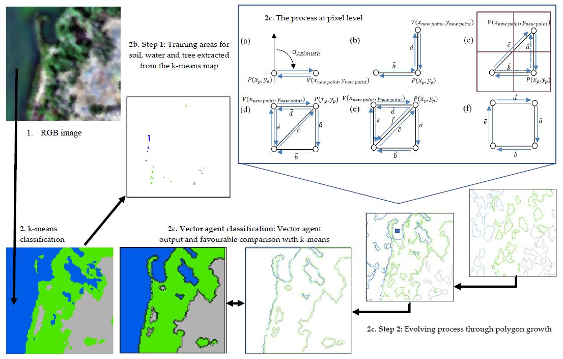
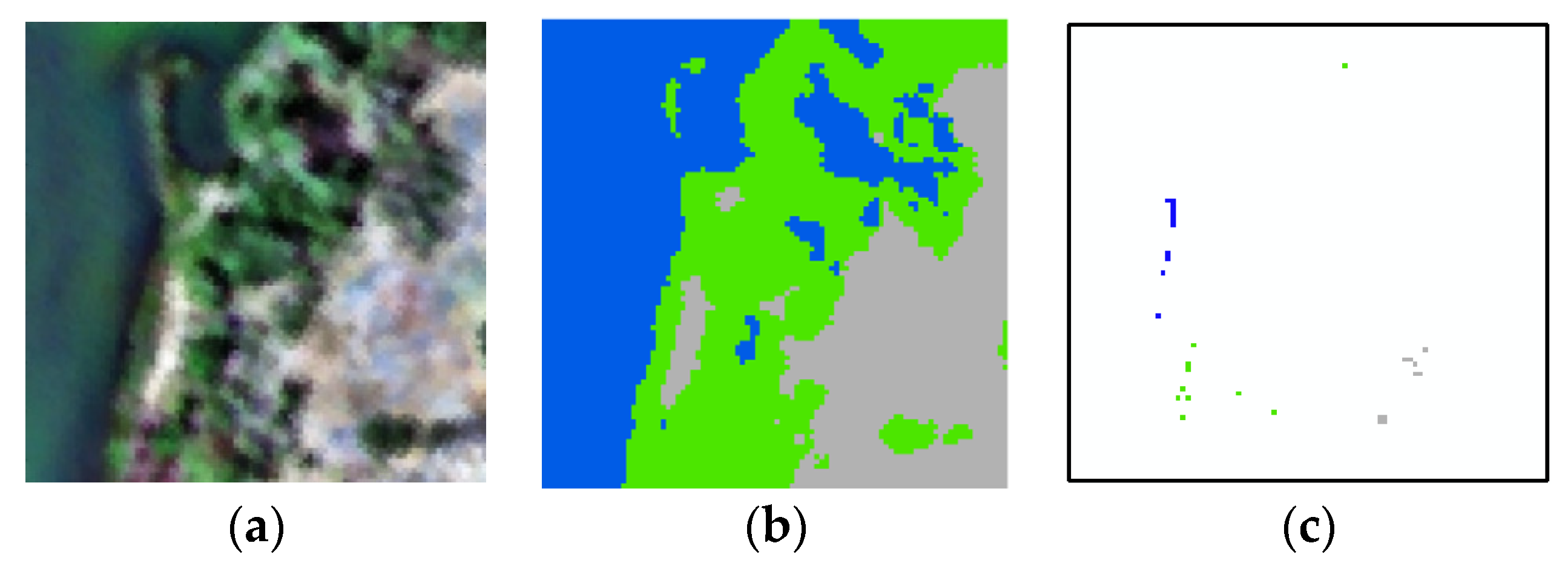
2.1. Creation of Training Samples
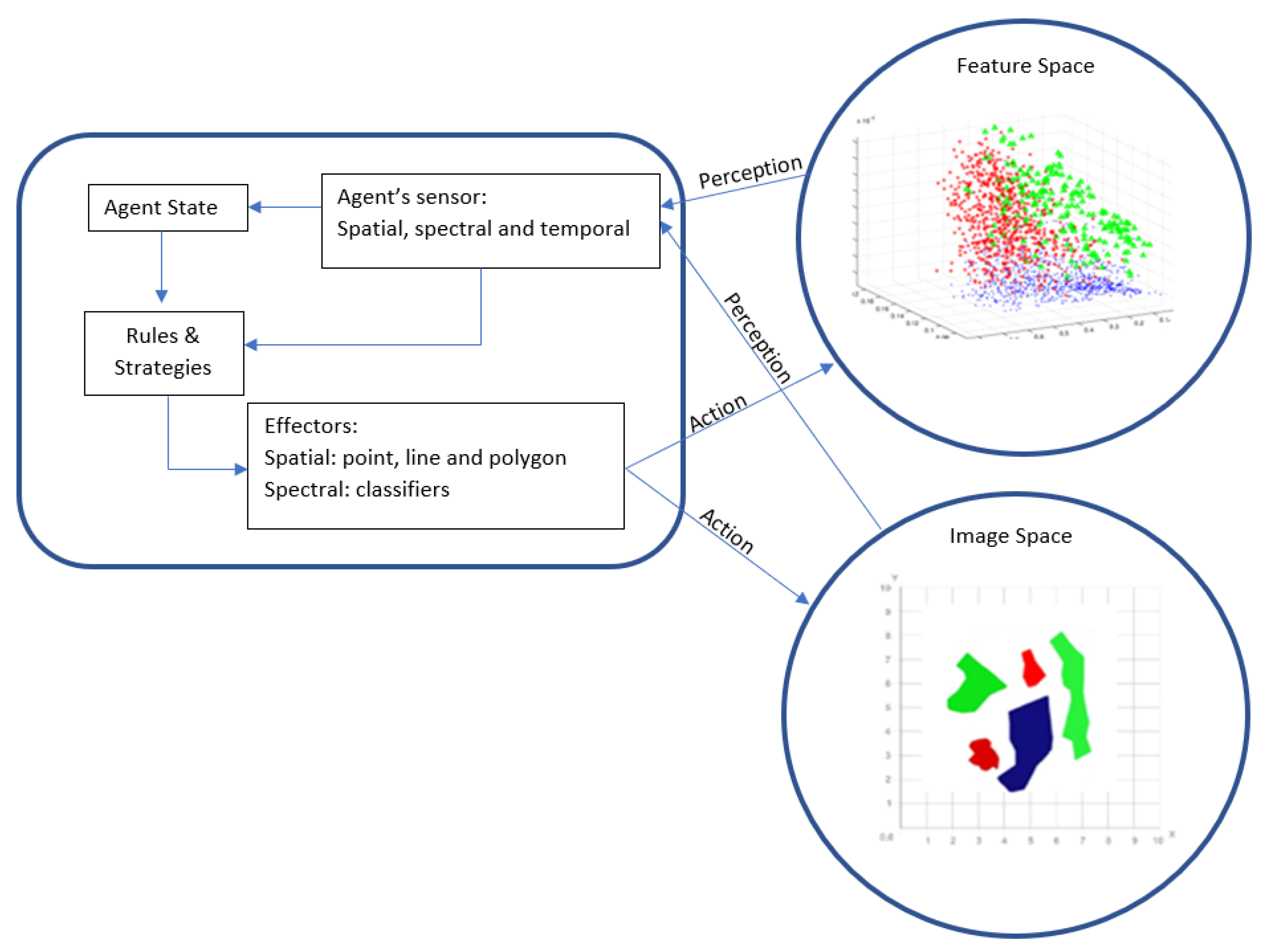
2.2. Construction of the VA Model
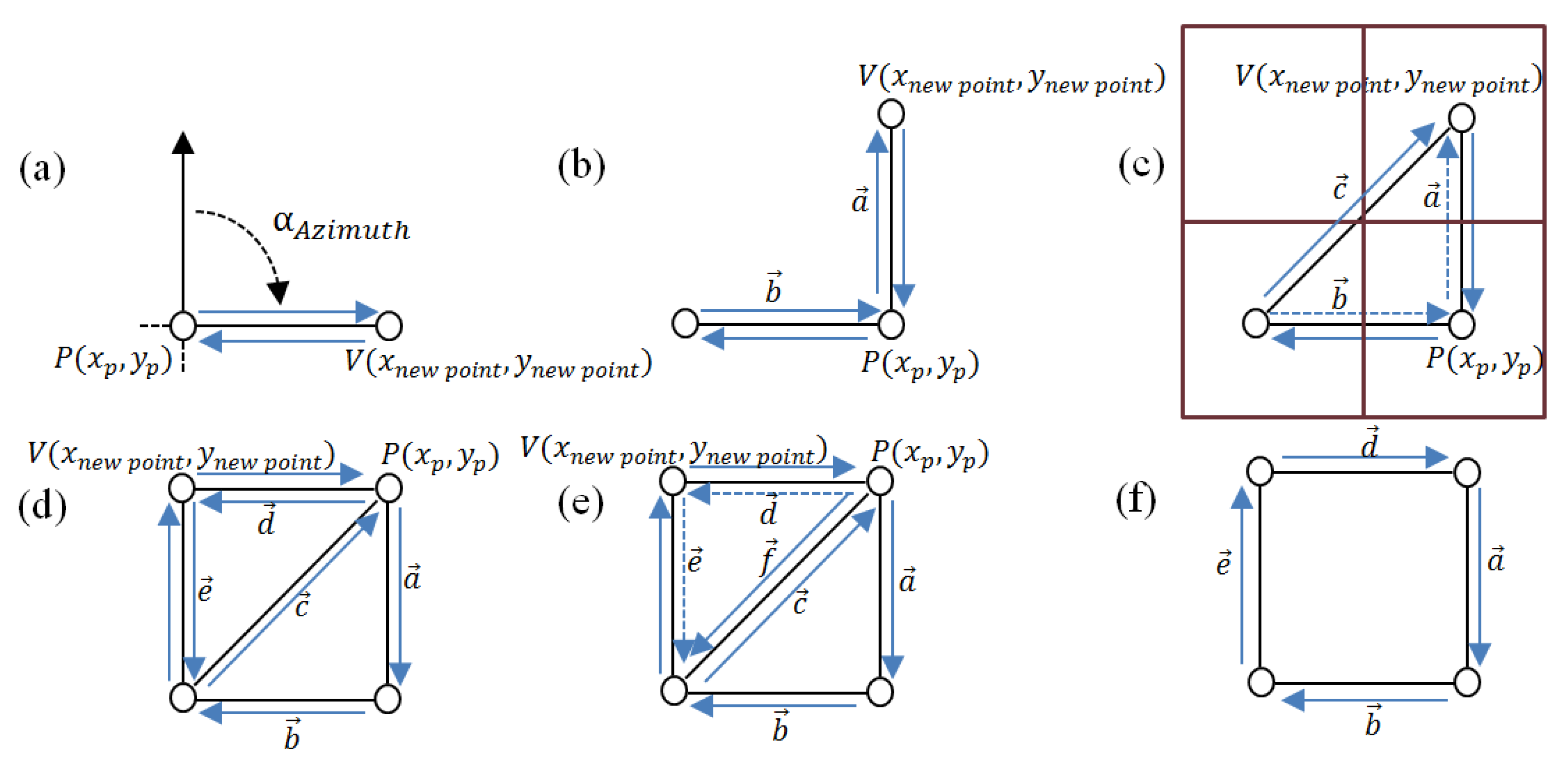
2.2.1. Geometry and Geometry Methods
- Vertex displacement: This places a new vertex and connects two vertices together by two half-edges, specified according to a single direction (Figure 3a,b);
- Converging vertex displacement: Two new edges are constructed to a single vertex form two existing neighbouring vertices (Figure 3c);
- Half-edge joining: This constructs a new edge based on a twin or bidirectional edge that is formed by two half-edges (Figure 3d);
- Edge remove: This forms a new polygon by merging two polygons (Figure 3f).
2.2.2. State and Transition Rules
- The candidate pixel xc and its immediate neighbours in the image must be members of the same class. VAs use the SVM classifier to evaluate such membership.
2.2.3. Neighbourhood and Neighbourhood Rules
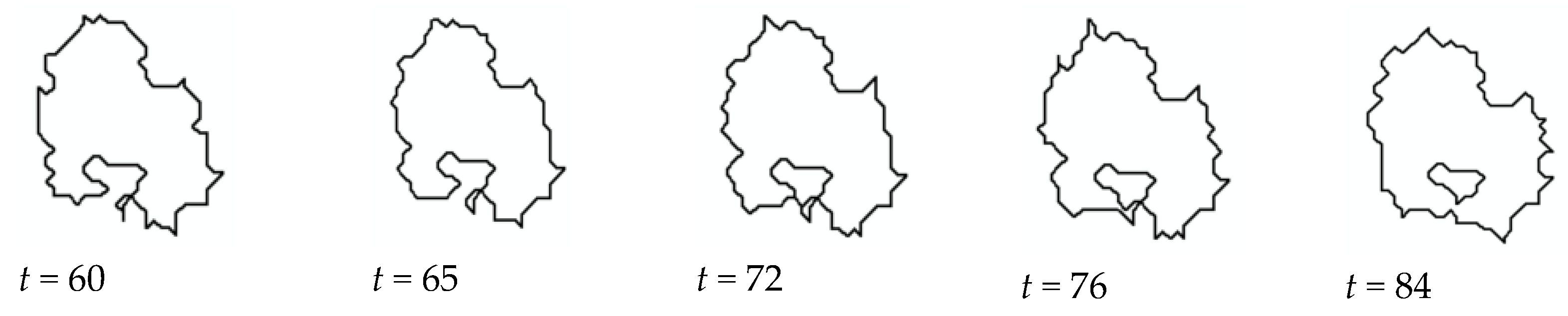
2.2.4. Implementation of VA for Unsupervised Classification
3. Experiments and Results
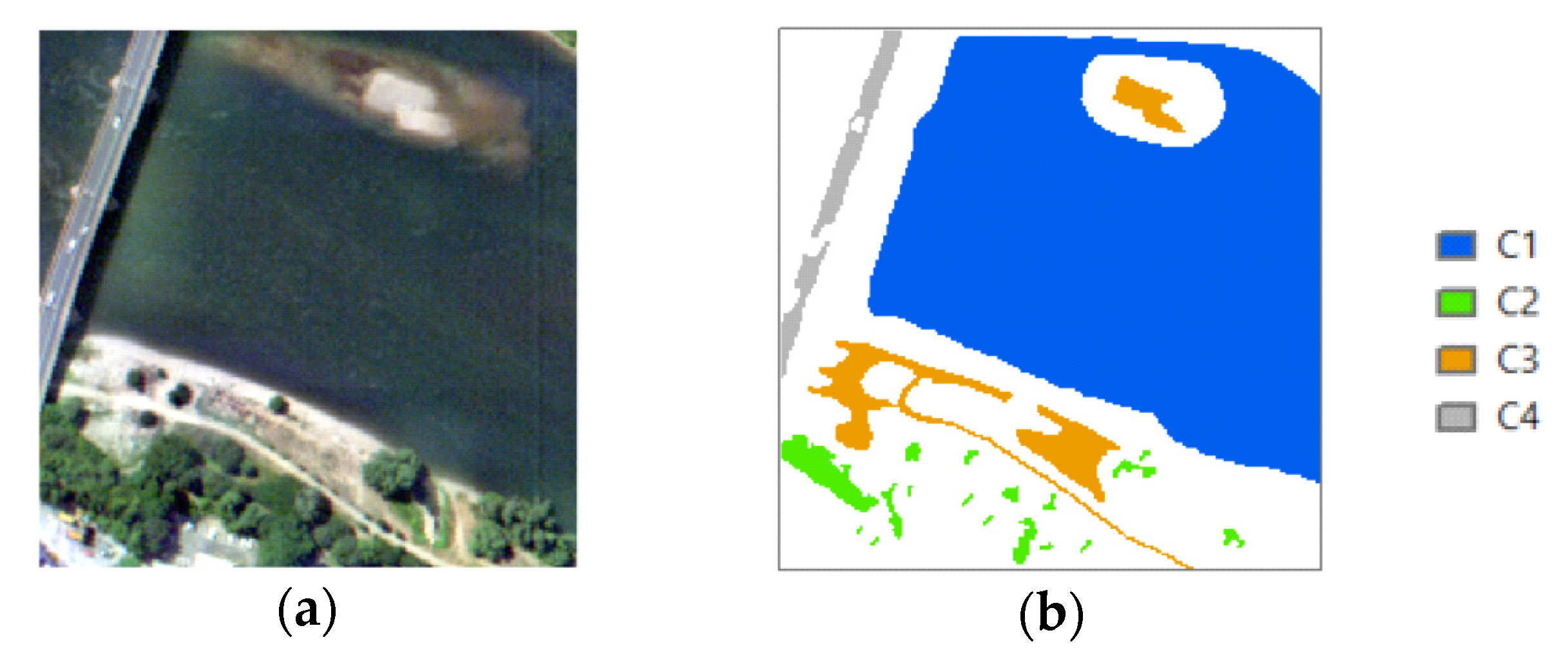
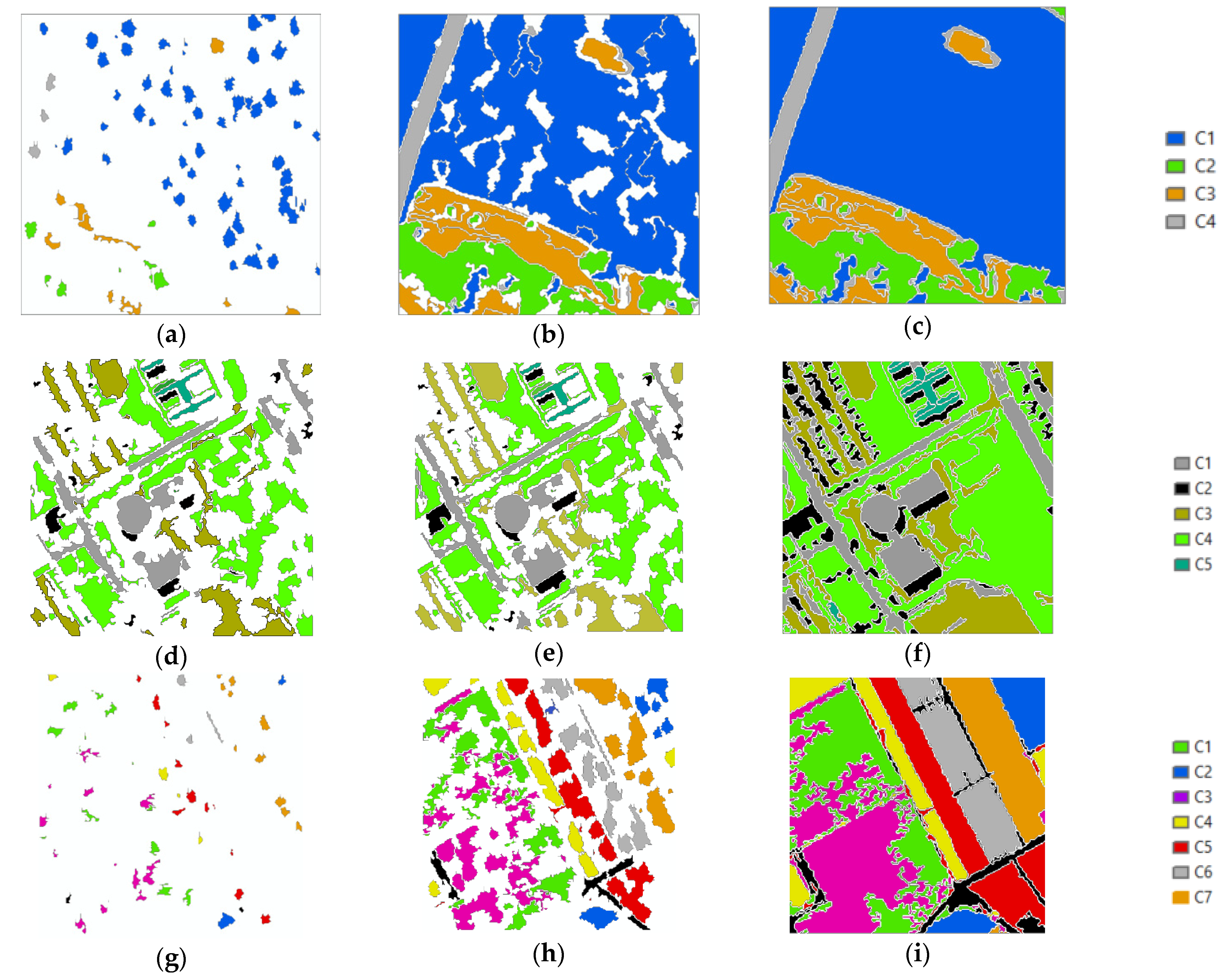
3.1. Datasets
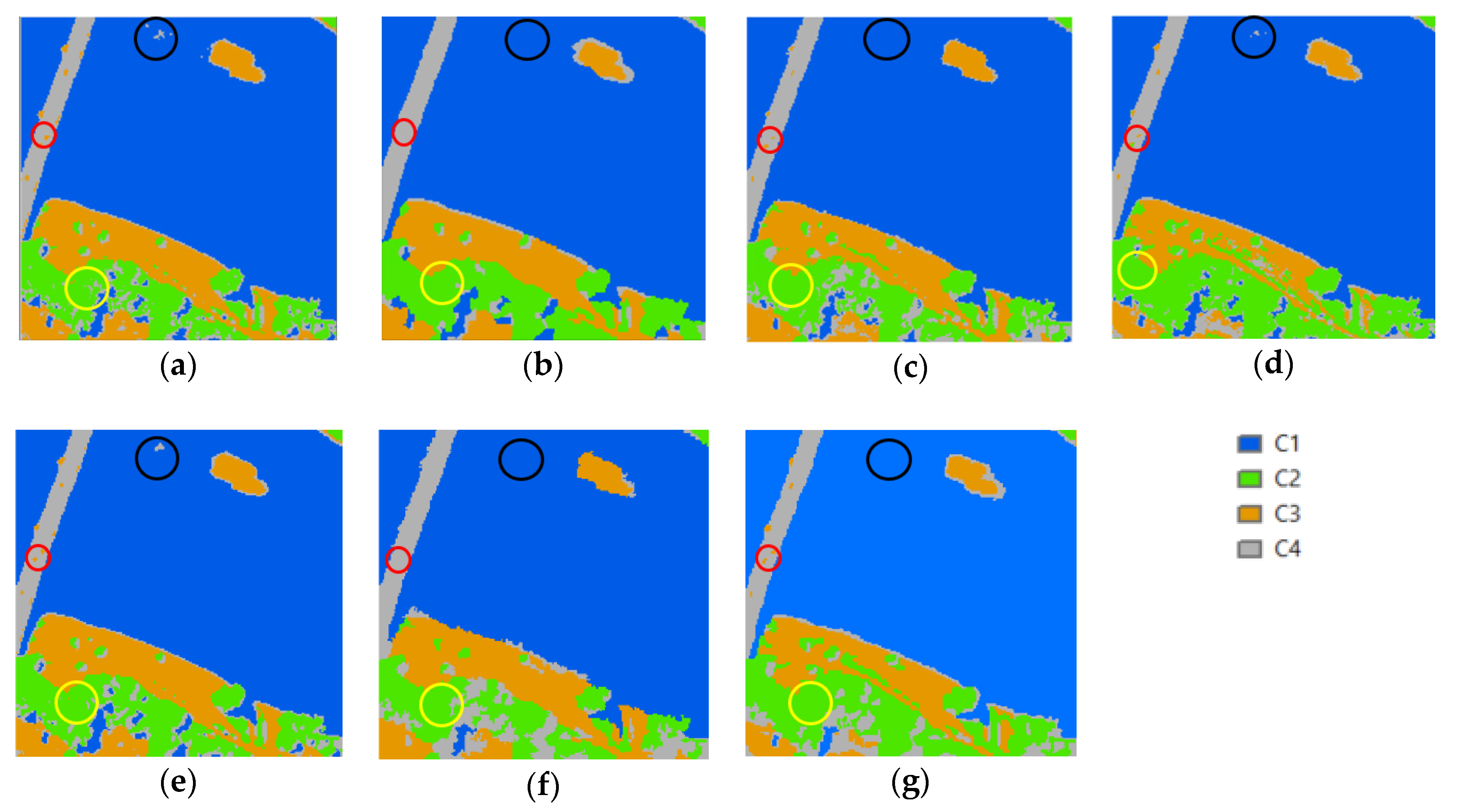
3.2. Image Clustering
- i.
- Unsupervised
- Spectral-Spatial classification (SSC)
- Majority Filtering (MF)
- ii.
- Semi-supervised
- SVM:
- Mean Shift Segmentation (MSS):
- Multiresolution Segmentation (MRS):
3.3. Evaluation Metrics
3.4. Results
4. Discussion
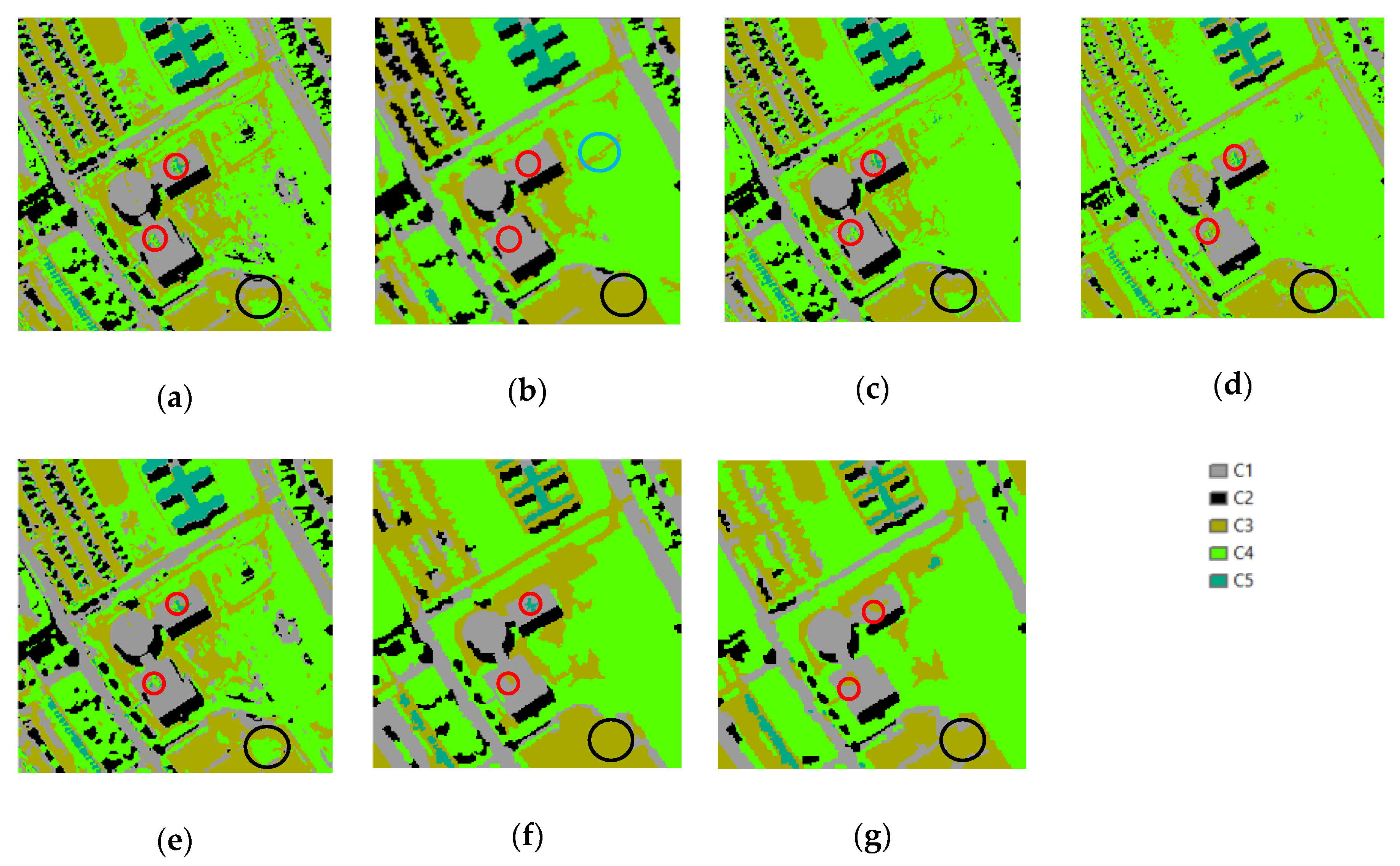
4.1. Dataset 1
4.1.1. Speckled Noise Analysis
4.1.2. Accuracy Analysis
4.2. Dataset 2
4.2.1. Speckled Noise Analysis
4.2.2. Accuracy Analysis
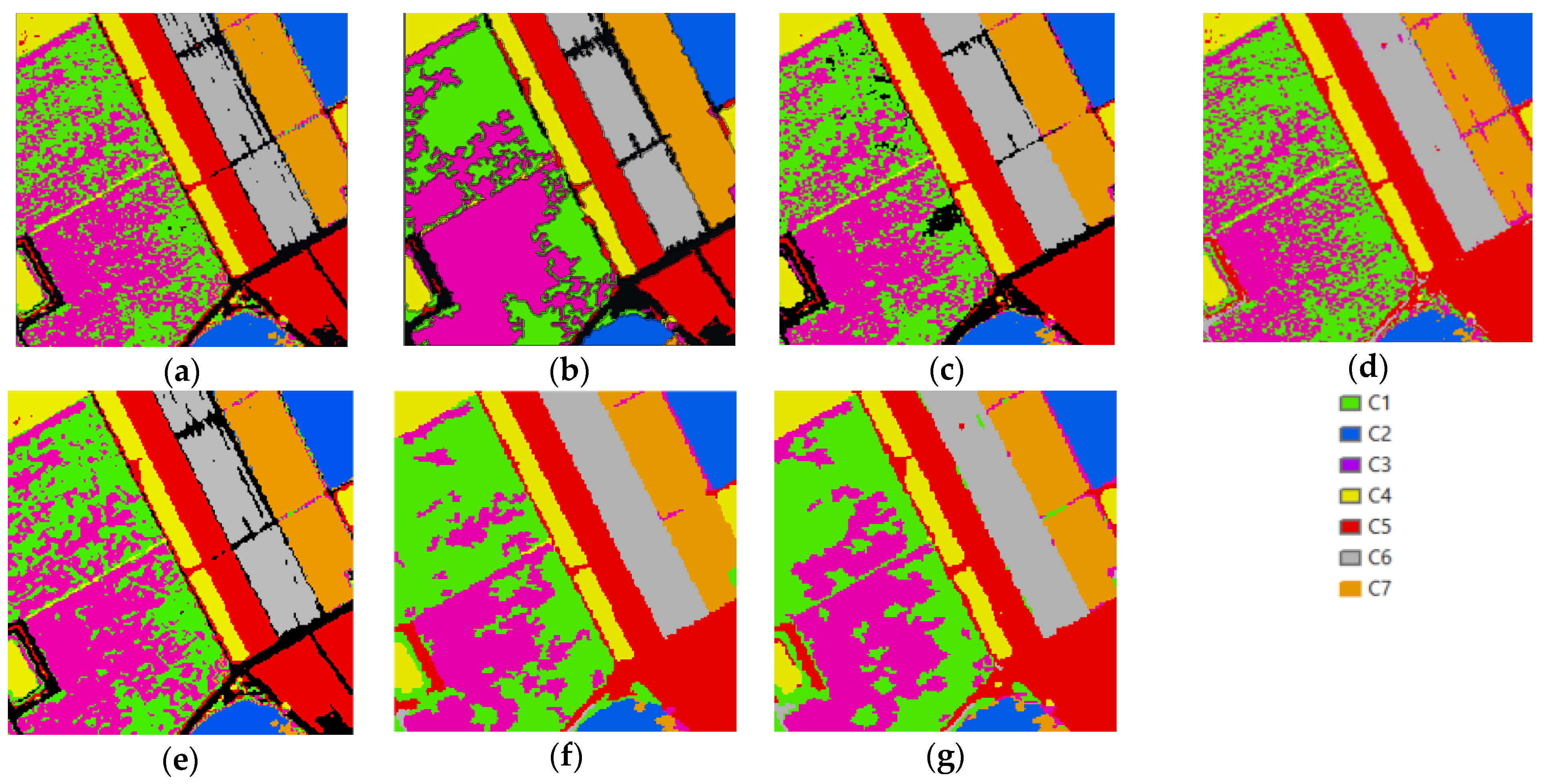
4.3. Dataset 3
4.3.1. Speckled Noise Analysis
4.3.2. Accuracy Analysis
5. Conclusions
Author Contributions
Funding
Institutional Review Board Statement
Informed Consent Statement
Data Availability Statement
Conflicts of Interest
References
- Tso, B.; Olsen, R.C. Combining spectral and spatial information into hidden Markov models for unsupervised image classification. Int. J. Remote Sens. 2005, 26, 2113–2133. [Google Scholar] [CrossRef]
- Madhu, A.; Kumar, A.; Jia, P. Exploring Fuzzy Local Spatial Information Algorithms for Remote Sensing Image Classification. Remote Sens. 2021, 13, 4163. [Google Scholar] [CrossRef]
- Tyagi, M.; Bovolo, F.; Mehra, A.K.; Chaudhuri, S.; Bruzzone, L. A context-sensitive clustering technique based on graph-cut initialisation and expectation-maximisation algorithm. IEEE Geosci. Remote Sens. Lett. 2008, 5, 21–25. [Google Scholar] [CrossRef] [Green Version]
- Madubedube, A.; Coetzee, S.; Rautenbach, V. A Contributor-Focused Intrinsic Quality Assessment of OpenStreetMap in Mozambique Using Unsupervised Machine Learning. ISPRS Int. J. Geo-Inf. 2021, 10, 156. [Google Scholar] [CrossRef]
- Chi, M.; Feng, R.; Bruzzone, L. Classification of hyperspectral remote-sensing data with primal SVM for small-sized training dataset problem. Adv. Space Res. 2008, 41, 1793–1799. [Google Scholar] [CrossRef]
- Ragettli, S.; Herberz, T.; Siegfried, T. An Unsupervised Classification Algorithm for Multi-Temporal Irrigated Area Mapping in Central Asia. Remote Sens. 2018, 10, 1823. [Google Scholar] [CrossRef] [Green Version]
- Ghaffarian, S.; Ghaffarian, S. Automatic histogram-based fuzzy C-means clustering for remote sensing imagery. ISPRS J. Photogramm. Remote Sens. 2014, 97, 46–57. [Google Scholar] [CrossRef]
- Tarabalka, Y.; Chanussot, J.; Benediktsson, J.A.; Angulo, J.; Fauvel, M. Segmentation and classification of hyperspectral data using watershed. In Proceedings of the IEEE International Geoscience and Remote Sensing Symposium; IEEE: Boston, MA, USA, 2008; pp. 652–655. [Google Scholar]
- Zheng, N.; Zhang, H.; Fan, J.; Guan, H. A fuzzy local neighbourhood-attraction-based information c-means clustering algorithm for very high spatial resolution imagery classification. Remote Sens. Lett. 2014, 5, 1328–1337. [Google Scholar] [CrossRef]
- Zhang, H.; Zhai, H.; Zhang, L.; Li, P. Spectral–Spatial Sparse Subspace Clustering for Hyperspectral Remote Sensing Images. IEEE Trans. Geosci. Remote Sens. 2016, 54, 3672–3684. [Google Scholar] [CrossRef]
- Cui, W.; Zhang, D.; He, X.; Yao, M.; Wang, Z.; Hao, Y.; Li, J.; Wu, W.; Cui, W.; Huang, J. Multi-Scale Remote Sensing Semantic Analysis Based on a Global Perspective. ISPRS Int. J. Geo-Inf. 2019, 8, 417. [Google Scholar] [CrossRef] [Green Version]
- Li, N.; Huo, H.; Zhao, Y.M.; Chen, X.; Fang, T. A spatial clustering method with edge weighting for image segmentation. Geosci. Remote Sens. Lett. 2013, 10, 1124–1128. [Google Scholar]
- Miao, Z.; Shi, W. A New Methodology for Spectral-Spatial Classification of Hyperspectral Images. J. Sens. 2016, 1–12. [Google Scholar] [CrossRef] [Green Version]
- Dzung, L. Pham, Spatial Models for Fuzzy Clustering. Comput. Vis. Image Underst. 2001, 84, 285–297. [Google Scholar]
- Hay, G.J.; Castilla, G.; Wulder, M.A.; Ruiz, J.R. An automated object-based approach for the multiscale image segmentation of forest scenes. Int. J. Appl. Earth Obs. Geoinf. 2005, 7, 339–359. [Google Scholar] [CrossRef]
- Tian, J.; Chen, D.M. Optimisation in multi-scale segmentation of high-resolution satellite images for artificial feature recognition. Int. J. Remote Sens. 2007, 28, 4625–4644. [Google Scholar] [CrossRef]
- Feizizadeh, B.; Garajeh, M.K.; Blaschke, T.; Lakes, T. An object based image analysis applied for volcanic and glacial landforms mapping in Sahand Mountain, Iran. Catena 2021, 198, 105073. [Google Scholar] [CrossRef]
- Kurtz, C.; Passat, N.; Gançarski, P.; Puissant, A. Multi-resolution region-based clustering for urban analysis. Int. J. Remote Sens. 2010, 31, 59415973. [Google Scholar] [CrossRef]
- Gençtav, A.; Aksoy, S.; Önder, S. Unsupervised segmentation and classification of cervical cell images. Pattern Recognit. 2012, 45, 4151–4168. [Google Scholar] [CrossRef] [Green Version]
- Hesheng, W.; Baowei, F. A modified fuzzy C-means classification method using a multiscale diffusion filtering scheme. Med. Image Anal. 2009, 13, 193–202. [Google Scholar]
- Fang, B.; Chen, G.; Chen, J.; Ouyang, G.; Kou, R.; Wang, L. CCT: Conditional Co-Training for Truly Unsupervised Remote Sensing Image Segmentation in Coastal Areas. Remote Sens. 2021, 13, 3521. [Google Scholar] [CrossRef]
- Yin, S.; Qian, Y.; Gong, M. Unsupervised hierarchical image segmentation through fuzzy entropy maximization. Pattern Recognit. 2017, 68, 245–259. [Google Scholar] [CrossRef]
- Hay, G.J.; Castilla, G. Geographic Object-Based Image Analysis (GEOBIA): A new name for a new discipline. In Object-Based Image Analysis; Springer: Berlin/Heidelberg, Germany, 2008; pp. 75–89. [Google Scholar]
- Baatz, M.; Hoffmann, C.; Willhauck, G. Progressing from object-based to object-oriented image analysis. In Object-Based Image Analysis; Springer: Berlin/Heidelberg, Germany, 2008; pp. 29–42. [Google Scholar]
- Blaschke, T.; Hay, G.J.; Kelly, M.; Lang, S.; Hofmann, P.; Addink, E.; Feitosa, R.Q.; van der Meer, F.; van der Werff, H.; van Coillie, F. Geographic object-based image analysis–towards a new paradigm. ISPRS J. Photogramm. Remote 2014, 87, 180–191. [Google Scholar] [CrossRef] [PubMed] [Green Version]
- Troya-Galvis, A.; Gançarski, P.; Berti-Équille, L. Remote sensing image analysis by aggregation of segmentation-classification collaborative agents. Pattern Recognit. 2018, 73, 259–274. [Google Scholar] [CrossRef]
- Hofmann, P.; Lettmayer, P.; Blaschke, T.; Belgiu, M.; Wegenkittl, S.; Graf, R.; Lampoltshammer, T.J.; Andrejchenko, V. Towards a framework for agent-based image analysis of remote-sensing data. Int. J. Image Data Fusion 2015, 6, 115–137. [Google Scholar] [CrossRef] [Green Version]
- Torrens, P.M.; Benenson, I. Geographic automata systems. Int. J. Geogr. Inf. Sci. 2005, 19, 385–412. [Google Scholar] [CrossRef] [Green Version]
- Hammam, Y.; Moore, A.; Whigham, P. The dynamic geometry of geographical vector agents. Comput. Environ. Urban Syst. 2007, 31, 502–519. [Google Scholar] [CrossRef]
- Chang, C.C.; Lin, C.J. LIBSVM: A Library for Support Vector Machines. ACM Trans. Intell. Systems Technol. 2011, 3, 1–27. [Google Scholar] [CrossRef]
- Moore, A. Geographical Vector Agent-Based Simulation for Agricultural Land Use Modelling. In Advanced Geosimulation Models; Marceau, D., Benenson, I., Eds.; 2011; pp. 30–48. Available online: http://www.casa.ucl.ac.uk/Advanced%20Geosimulation%20Models.pdf (accessed on 15 November 2021).
- Howe, T. Containing agents: Contexts, projections, and agents. In Proceedings of the Agent Conference on Social Agents: Results and Prospects; Argonne National Laboratory: Argonne, IL, USA, 2006. [Google Scholar]
- Borna, K.; Moore, A.B.; Sirguey, P. Towards a vector agent modelling approach for remote sensing image classification. J. Spat. Sci. 2014, 59, 283–296. [Google Scholar] [CrossRef]
- Borna, K.; Moore, A.B.; Sirguey, P. An Intelligent Geospatial Processing Unit for Image Classification Based on Geographic Vector Agents (GVAs). Trans. GIS 2016, 20, 368–381. [Google Scholar] [CrossRef]
- Mahmoudi, F.T.; Samadzadegan, F.; Reinartz, P. Object oriented image analysis based on multi-agent recognition system. Comput. Geosci. 2013, 54, 219–230. [Google Scholar] [CrossRef]


| Class | Metrics | k-Means | SSC | SVM | VA | MF | MSS | MRS |
|---|---|---|---|---|---|---|---|---|
| C1 | precision | 100.00 | 100.00 | 100.00 | 100.00 | 100.00 | 100.00 | 100.00 |
| Jaccard-index | 99.88 | 100.00 | 99.95 | 100.00 | 99.91 | 100.00 | 99.99 | |
| F-score | 99.94 | 100.00 | 99.98 | 100.00 | 99.96 | 100.00 | 100.00 | |
| recall | 99.88 | 100.00 | 99.95 | 100.00 | 99.91 | 100.00 | 99.99 | |
| C2 | precision | 100.00 | 99.86 | 94.29 | 99.46 | 99.87 | 100.00 | 98.28 |
| Jaccard-index | 98.25 | 98.79 | 94.17 | 99.20 | 99.60 | 94.35 | 98.15 | |
| F-score | 99.12 | 99.39 | 97.00 | 99.60 | 99.80 | 97.10 | 99.07 | |
| recall | 98.25 | 98.92 | 99.87 | 99.73 | 99.73 | 94.35 | 99.87 | |
| C3 | precision | 99.94 | 100.00 | 100.00 | 100.00 | 100.00 | 100.00 | 99.88 |
| Jaccard-index | 99.94 | 99.83 | 93.94 | 99.77 | 99.94 | 98.04 | 99.14 | |
| F-score | 99.97 | 99.91 | 96.88 | 99.88 | 99.97 | 99.01 | 99.57 | |
| recall | 100.00 | 99.83 | 93.94 | 99.77 | 99.94 | 98.04 | 99.25 | |
| C4 | precision | 95.22 | 98.66 | 91.34 | 99.73 | 97.49 | 93.89 | 91.34 |
| Jaccard-index | 95.10 | 98.66 | 91.34 | 99.73 | 97.49 | 93.89 | 91.34 | |
| F-score | 97.49 | 99.33 | 95.47 | 99.86 | 98.73 | 96.85 | 95.47 | |
| recall | 99.86 | 100.00 | 100.00 | 100.00 | 100.00 | 100.00 | 100.00 | |
| C1–4 | OA | 99.83 | 99.95 | 99.49 | 99.97 | 99.91 | 99.66 | 99.93 |
| Method | SSC | VA | MSS | MRS | ||||
|---|---|---|---|---|---|---|---|---|
| Class | C2 | C3 | C2 | C3 | C2 | C3 | C2 | C3 |
| Number | 37 | 26 | 11 | 6 | 15 | 6 | 22 | 16 |
| Area (m2) | 8549.85 | 9621.59 | 9335.86 | 9820.32 | 7479.82 | 10,263.82 | 10,225.76 | 7947.24 |
| Perimeter (m) | 2513.01 | 2089.01 | 1533.01 | 1379.62 | 1855.19 | 1599.30 | 2282.84 | 1787.64 |
| P/A ratio | 0.29 | 0.21 | 0.16 | 0.14 | 0.25 | 0.16 | 0.22 | 0.22 |
| Class | Metrics | k-Means | SSC | SVM | VA | MF | MSS | MRS |
|---|---|---|---|---|---|---|---|---|
| C1 | precision | 76.82 | 87.69 | 99.38 | 93.24 | 73.25 | 78.86 | 87.14 |
| Jaccard-index | 75.41 | 87.19 | 82.55 | 92.75 | 68.36 | 72.43 | 81.85 | |
| F-score | 85.98 | 93.16 | 90.44 | 96.24 | 81.21 | 84.01 | 90.02 | |
| recall | 97.62 | 99.35 | 82.98 | 99.44 | 91.10 | 89.89 | 93.09 | |
| C2 | precision | 71.05 | 97.85 | 100 | 98.15 | 61.07 | 79.08 | 98.55 |
| Jaccard-index | 71.05 | 97.85 | 100 | 98.15 | 58.55 | 73.48 | 84.21 | |
| F-score | 83.07 | 98.91 | 100 | 99.07 | 73.85 | 84.72 | 91.43 | |
| recall | 100 | 100 | 100 | 100 | 93.42 | 91.22 | 85.27 | |
| C3 | precision | 46.46 | 52.12 | 68.14 | 55.43 | 38.41 | 27.94 | 44.27 |
| Jaccard-index | 42.47 | 43.98 | 67.64 | 52.01 | 32.48 | 21.23 | 37.35 | |
| F-score | 59.62 | 61.09 | 80.7 | 68.43 | 49.03 | 35.02 | 54.39 | |
| recall | 83.16 | 73.79 | 98.93 | 89.40 | 67.79 | 46.92 | 70.50 | |
| C4 | precision | 99.78 | 99.78 | 99.79 | 99.87 | 96.83 | 95.05 | 94.95 |
| Jaccard-index | 67.63 | 84.2 | 97.38 | 82.96 | 65.72 | 74.05 | 78.84 | |
| F-score | 80.69 | 91.42 | 98.67 | 90.69 | 79.32 | 85.09 | 88.17 | |
| recall | 67.73 | 84.36 | 97.58 | 83.05 | 67.17 | 77.01 | 82.29 | |
| C5 | precision | 98.53 | 97.8 | 97.75 | 100 | 89.94 | 97.75 | 87.77 |
| Jaccard-index | 97.99 | 97.09 | 87.07 | 99.44 | 78.81 | 63.74 | 62.14 | |
| F-score | 98.98 | 98.52 | 93.09 | 99.72 | 88.15 | 77.85 | 76.65 | |
| recall | 99.44 | 99.26 | 88.85 | 99.44 | 86.43 | 64.68 | 68.03 | |
| C1–5 | OA | 79.56 | 87.93 | 93.88 | 89.19 | 74.85 | 76.10 | 82.69 |
| Method | SSC | VA | MSS | MRS | ||||
|---|---|---|---|---|---|---|---|---|
| Class | C1 | C4 | C1 | C4 | C1 | C4 | C1 | C4 |
| Number | 342 | 370 | 40 | 39 | 21 | 28 | 18 | 24 |
| Area (m2) | 13,850.52 | 38,233.43 | 13,555.06 | 36,978.89 | 13,146.53 | 38,329.54 | 13,824.32 | 40,807.29 |
| Perimeter (m) | 7083.78 | 11,199.85 | 4140.10 | 6285.49 | 3123.36 | 5586.51 | 3762.62 | 5619.38 |
| P/A ratio | 0.51 | 0.29 | 0.30 | 0.17 | 0.23 | 0.22 | 0.30 | 0.17 |
| Class | Metrics | k-Means | SSC | SVM | VA | MF | MSS | MRS |
|---|---|---|---|---|---|---|---|---|
| C1 | precision | 58.34 | 61.83 | 54.83 | 65.51 | 61.6 | 63.58 | 62.23 |
| Jaccard-index | 41.26 | 45.74 | 41.87 | 48.04 | 43.19 | 56.47 | 49.15 | |
| F-score | 58.41 | 62.77 | 59.02 | 64.9 | 60.33 | 72.18 | 65.9 | |
| Recall | 58.49 | 63.75 | 63.91 | 64.31 | 59.1 | 83.46 | 70.03 | |
| C2 | Precision | 98.92 | 100 | 100 | 100 | 96.5 | 100 | 100 |
| Jaccard-index | 90.32 | 88.22 | 88.42 | 94.81 | 90.54 | 88.22 | 86.63 | |
| F-score | 94.91 | 93.74 | 93.86 | 97.34 | 95.04 | 93.74 | 92.83 | |
| Recall | 91.22 | 88.22 | 88.42 | 94.81 | 93.61 | 88.22 | 86.63 | |
| C3 | Precision | 65.27 | 68.58 | 64.3 | 70.84 | 66.47 | 80.95 | 71.78 |
| Jaccard-index | 48.2 | 51.09 | 42.69 | 55.33 | 50.98 | 51.46 | 50.76 | |
| F-score | 65.05 | 67.63 | 59.84 | 71.25 | 67.53 | 67.95 | 67.34 | |
| Recall | 64.83 | 66.7 | 55.95 | 71.66 | 68.62 | 58.55 | 63.42 | |
| C4 | Precision | 97.93 | 97.54 | 98.56 | 97.39 | 86.45 | 86.33 | 86.69 |
| Jaccard-index | 96.21 | 96.99 | 96.82 | 96.65 | 77.68 | 82.02 | 79.92 | |
| F-score | 98.07 | 98.47 | 98.38 | 98.29 | 87.44 | 90.12 | 88.84 | |
| Recall | 98.21 | 99.43 | 98.21 | 99.21 | 88.45 | 94.26 | 91.1 | |
| C5 | Precision | 97.6 | 98.36 | 96.48 | 98.39 | 93.74 | 91.21 | 90.65 |
| Jaccard-index | 96.71 | 97.2 | 95.78 | 97.23 | 87.45 | 84.71 | 84.63 | |
| F-score | 98.33 | 98.58 | 97.85 | 98.6 | 93.30 | 91.72 | 91.67 | |
| Recall | 99.06 | 98.80 | 99.25 | 98.80 | 92.87 | 92.23 | 92.72 | |
| C6 | Precision | 100.00 | 100.00 | 99.75 | 99.97 | 100.00 | 99.70 | 99.44 |
| Jaccard-index | 99.88 | 99.84 | 99.42 | 99.89 | 100.00 | 99.45 | 98.67 | |
| F-score | 99.94 | 99.92 | 99.71 | 99.94 | 100.00 | 99.72 | 99.33 | |
| Recall | 99.88 | 99.84 | 99.67 | 99.92 | 100.00 | 99.75 | 99.22 | |
| C7 | Precision | 98.16 | 98.35 | 98.50 | 99.24 | 98.82 | 98.41 | 98.19 |
| Jaccard-index | 97.40 | 97.70 | 95.02 | 99.13 | 98.35 | 98.25 | 97.84 | |
| F-score | 98.68 | 98.83 | 97.45 | 99.56 | 99.17 | 99.12 | 98.91 | |
| recall | 99.21 | 99.32 | 96.42 | 99.89 | 99.52 | 99.83 | 99.63 | |
| C1–7 | OA | 75.91 | 78.04 | 76.34 | 80.01 | 76.79 | 81.69 | 79.52 |
| Method | SSC | VA | MSS | MRS | ||||
|---|---|---|---|---|---|---|---|---|
| Class | C1 | C3 | C1 | C3 | C1 | C3 | C1 | C3 |
| Number | 316 | 268 | 15 | 19 | 15 | 23 | 34 | 29 |
| Area (m2) | 104,838.89 | 119,822.50 | 102,764.97 | 126,549.36 | 147,059.32 | 93,143.21 | 128,887.22 | 114,776.89 |
| Perimeter (m) | 21,978.94 | 21,326.96 | 9577.48 | 9372.53 | 9001.97 | 7772.15 | 9153.52 | 8030.08 |
| P/A ratio | 0.21 | 0.18 | 0.09 | 0.07 | 0.06 | 0.08 | 0.07 | 0.07 |
Publisher’s Note: MDPI stays neutral with regard to jurisdictional claims in published maps and institutional affiliations. |
© 2021 by the authors. Licensee MDPI, Basel, Switzerland. This article is an open access article distributed under the terms and conditions of the Creative Commons Attribution (CC BY) license (https://creativecommons.org/licenses/by/4.0/).
Share and Cite
Borna, K.; Moore, A.B.; Noori Hoshyar, A.; Sirguey, P. Using Vector Agents to Implement an Unsupervised Image Classification Algorithm. Remote Sens. 2021, 13, 4896. https://doi.org/10.3390/rs13234896
Borna K, Moore AB, Noori Hoshyar A, Sirguey P. Using Vector Agents to Implement an Unsupervised Image Classification Algorithm. Remote Sensing. 2021; 13(23):4896. https://doi.org/10.3390/rs13234896
Chicago/Turabian StyleBorna, Kambiz, Antoni B. Moore, Azadeh Noori Hoshyar, and Pascal Sirguey. 2021. "Using Vector Agents to Implement an Unsupervised Image Classification Algorithm" Remote Sensing 13, no. 23: 4896. https://doi.org/10.3390/rs13234896
APA StyleBorna, K., Moore, A. B., Noori Hoshyar, A., & Sirguey, P. (2021). Using Vector Agents to Implement an Unsupervised Image Classification Algorithm. Remote Sensing, 13(23), 4896. https://doi.org/10.3390/rs13234896