Synergy of Sentinel-1 and Sentinel-2 Imagery for Early Seasonal Agricultural Crop Mapping

Abstract

The exploitation of the unprecedented capacity of Sentinel-1 (S1) and Sentinel-2 (S2) data offers new opportunities for crop mapping. In the framework of the SenSAgri project, this work studies the synergy of very high-resolution Sentinel time series to produce accurate early seasonal binary cropland mask and crop type map products. A crop classification processing chain is proposed to address the following: (1) high dimensionality challenges arising from the explosive growth in available satellite observations and (2) the scarcity of training data. The two-fold methodology is based on an S1-S2 classification system combining the so-called soft output predictions of two individually trained classifiers. The performances of the SenSAgri processing chain were assessed over three European test sites characterized by different agricultural systems. A large number of highly diverse and independent data sets were used for validation experiments. The agreement between independent classification algorithms of the Sentinel data was confirmed through different experiments. The presented results assess the interest of decision-level fusion strategies, such as the product of experts. Accurate crop map products were obtained over different countries in the early season with limited training data. The results highlight the benefit of fusion for early crop mapping and the interest of detecting cropland areas before the identification of crop types.

1. Introduction

Cropland and crop type maps at global and regional scales provide critical information for agricultural monitoring systems. Satellite-derived remotely sensed data are proven to be an effective tool for crop type identification and spatial mapping. Nevertheless, the operational production of upscaling and delivering reliable and timely crop map products is challenging. Agricultural areas are complex landscapes characterized by many wide-ranging cropping systems, crop species and varieties. Another source of difficulty is the high diversity of existing agricultural practices (e.g., multiple within-year cropping), pedoclimatic conditions and geographical environments.

Crop mapping methods based on remote sensing exploit the spatiotemporal information of satellite image time series. The accurate recognition of crops requires high-quality spatial and temporal data [1,2,3]. In practice, the resolutions of satellite imagery will limit the accuracy of crop map products and their corresponding class legends [4]. Cropland extent knowledge is usually obtained from global maps, such as Moderate Resolution Imaging Spectroradiometer (MODIS) land cover [5], the Globland 30 m [6] or the GlobCover [7]. Unfortunately, these products do not always provide reliable information given the large disagreements and uncertainties existing among them [8,9,10]. In addition, their quality is far from satisfactory for applications requiring up-to-date accurate knowledge about food production or environmental issues. Therefore, accurate and timely crop information is still required for government decision making and agricultural management. Ideally, the user community has expressed the need for near-real-time high spatial resolution crop type maps from the early season [11].

In recent years, new high-resolution image time series have been acquired by the Sentinel mission under the EU’s Copernicus environmental monitoring program. SAR and optical data with high revisit frequency and large spatial coverage have become freely available thanks to the launch of the European Space Agency (ESA)’s Sentinel-1 and Sentinel-2 satellites. The high resolutions of these complementary satellite data present unprecedented opportunities for regional and global agriculture monitoring.

Although Sentinel-2 offers many opportunities for characterizing the spectral reflectance properties of crops [12], its temporal resolution can be limited. Cloud coverage can strongly affect important key data during the agricultural season or create consistent cloud-covered areas. Under this situation, Sentinel-1 images that are not affected by cloudy weather conditions can provide valuable complementary information. In addition, SAR images can help to discriminate between different crop types having similar spectro-temporal profiles [13]. The benefits of Sentinel-1 images can be reduced due to the presence of speckle noise. The high radar sensitivity to soil moisture may also complicate the interpretation of information from vegetation. Fluctuations induced by speckle or moisture changes (e.g., rain or snow) can then be confused with vegetation growth changes.

Operational large-scale crop monitoring methods need to satisfy some well-known requirements, such as cost-effectiveness, a high degree of automation, transferability and genericity. In this framework, the European H2020 Sentinels Synergy for Agriculture (SenSAgri) projet [14] has been proposed to demonstrate the benefit of the combined Sentinel -1 and -2 missions to develop an innovative portfolio of prototype agricultural monitoring services. In this project, the synergy of optical and radar monitoring was exploited to develop three prototype services capable of near-real-time operations: (1) surface soil moisture (SSM), (2) green and brown leaf area index (LAI) and (3) in-season crop mapping. Different European test sites covering different areas and agricultural practices have been used for method development, prototyping and validation.

The work presented here describes the research conducted in the SenSAgri project to develop a new processing chain for in-season crop mapping. From the early season, the innovative crop mapping chain exploits Sentinel-1 and -2 data to produce seasonal binary cropland masks and crop type maps. The two crop products are generated with a spatial resolution of 10 meters, and they follow the product specifications proposed by the Sen2-Agri system [15]. The proposed methodology aims to face the challenges of high-dimensional Sentinel data classification. Different experiments are presented in this work to assess (1) the crop mapping performances of the SenSAgri processing chain and (2) the synergy and complementarity of Sentinel’s data, showing the interest of fusing both data types. The main contributions of this study are as follows:

• It presents a robust and largely validated crop classification system to produce accurate crop map products in the early season with limited training data;
• It highlights the benefit of postdecision fusion strategies to exploit the synergy and complementarity among classifiers trained with Sentinel-1 (S1) and Sentinel-2 (S2) time series. This demonstrates the limitations of the early fusion method for classifying multimodal high-dimensional Sentinel time series;
• It confirms the interest of detecting cropland areas before the identification of crop types. A strategy for binary cropland area detection is proposed to reduce the impact of land cover legend definition on crop classification results.

This paper is organized as follows: Section 2 reviews the state-of-the-art classification strategies for crop mapping. Section 3 details the SenSagri methodology and, more precisely, the S1-S2 classification scheme and input features; Section 4 describes the satellite and reference data; Section 5 and Section 6 are devoted to the results and discussions; and finally, Section 7 draws the conclusions.

2. Related Work

The classification of multitemporal data by algorithms trained on user knowledge has been commonly proposed in the crop mapping literature. The classification results of these methods are noticeably impacted by the choice of the supervised classifier, the input data, the legend (details and number of classes) and the reference data [16]. Ideally, the quantity and quality of reference data need to ensure the diversity of the classification problem to ensure the generalization of the learned models.

Despite the large family of existing crop classification methods, most of them are not scalable. In practice, they have been tested on tiny test sites over restricted geographical areas. In addition, most of the existing classification methodologies have not considered natural vegetation classes such as grassland or shrubland, which are mostly confused with crop classes. In the same direction, classical land cover classification methodologies (see [17] for a review) do not generally satisfy the needs of operational agricultural monitoring requirements [18].

Traditionally, optical data with low and moderate resolutions have been exploited for large-scale crop mapping. The high temporal resolution of MODIS has shown an obvious benefit for the characterization of vegetation surfaces. Numerous crop mapping works have thus highlighted the usefulness of the normalized difference vegetation index (NDVI) derived from MODIS. Several works, such as [19,20,21], have proposed applying the decision tree (DT) classifier to MODIS data. These low-resolution multitemporal data have also been classified by other strategies based on the Jeffries–Matusita distance [22] or k mean [23]. Unfortunately, median resolution satellite data, such as MODIS, are too coarse to capture detailed crop information due to mixed land covers or land uses.

Several works have proposed combining the temporal information of MODIS with high-spatial resolution data. For instance, a DT methodology was proposed in [24] to reach 30 m crop maps by combining cropland MODIS 250 m products with LANDSAT data. The combination of MODIS and LANDSAT data has also been proposed by the US Cropland Data Layer [25,26], which is produced by the United States Department of Agriculture (USDA) and the National Agricultural Statistics Service (NASS). The accurate performances of this last DT methodology can be explained by the extensive use of parcel-level information provided by farmers’ declarations. SPOT data have also been combined with MODIS in [27], where an SVM joint classifier is applied to temporal NDVI features. The interest of incorporating ancillary data with multiple input satellite datasets in the classification process has also been highlighted in [28]. In this last work, crop maps with low spatial resolution were obtained by applying a spectral correlation classification strategy. The combination of Landsat and Sentinel-2 has been recently proposed in [15,29]. In this last work, the use of NDVI phenological metrics derived from high-spatial resolution datasets was investigated.

Some works have proposed combining the prediction of several DT classifiers, which are trained on different sets of satellite-derived features [20,30]. The high performances of classifier ensemble strategies have been confirmed in recent decades by the use of random forest (RF) classifiers. The robustness of RF to classify multitemporal satellite data over large geographical areas has been proposed in several studies [31,32,33]. The short training time, easy parameterization and high robustness to high-dimensional input features explain why RF has witnessed a growing interest in crop classification. Some works have applied RF to Landsat multiyear time series composites [34] and satellite-derived EVI time series [35]. More recently, pixel-wise [36] and object-based crop mapping methods [37] have also been proposed to classify Sentinel-2 data.

In recent years, deep learning (DL) classification strategies have been proposed for crop classification. Different deep architectures have been evaluated on very restricted geographical areas by some promising works. Some interesting examples of deep architectures are LSTM [38,39], transformers [40] and 3D-CNN [41]. Model transferability, the handling of spatial context with complex semantic models and the high semantic (categorial) resolution of mapping applications are some advantages highlighted by the use of CNN. However, these architectures do not exploit the spatiotemporal features of the data. The design of architectures capturing spatiotemporal information involves multiple options that are nontrivial and expensive to evaluate. Despite the unreasonable effectiveness of DL methodologies, they still involve important challenges for operational global crop mapping systems [42], including the requirement of a large amount of field data. Unfortunately, the scarcity of reference data is a well-known challenge for operational remote sensing applications. The obtention of crop and non-crop reference data over large-scale areas can be tedious. In addition, such data is not available in a timely fashion during the agricultural season and can contain class label noise. On the other hand, DL methods are also computationally expensive, and they require large computational operations in terms of memory. Last, these methods are usually patch-based approaches, and the patch size definition has negative impacts on object classification results.

From an operational point of view, the use of RF for classifying Sentinel-2 data has been assessed by the Sen2Agri project [15,43,44]. This operational processing chain has proposed an accurate two-fold methodology for producing binary cropland masks and crop type maps. Despite the satisfactory accuracies obtained by the Sen2Agri system, the crop mapping methodology has some limitations. First, the phenological metrics proposed for binary cropland masking can lead to a performance decrease for large-scale mapping [32]. Second, the proposed binary classification methodology requires the construction of a non-crop reference dataset, which can be very challenging. Last, Sen2Agri products are strongly dependent on the availability of Sentinel-2 acquisitions. Therefore, less accurate results are obtained in cloudy areas.

As previously mentioned, the integration of weather-independent synthetic aperture radar (SAR) imagery into crop classification methodologies may be a solution to address the lack of optical data. The use of multitemporal SAR data has gained increasing attention in crop monitoring [45,46]. Recently, the multisite crop classification experiment described in [47] proved the good performance of the RF classifier on multitemporal SAR data.

In the context of land use mapping and monitoring, the fusion of optical and radar data has been reviewed by different studies [48,49,50]. Despite the large number of such studies, most of the existing approaches do not consider the temporal dimension, and only a few images are fused. The most widely used strategy for exploiting multimodal time series is early fusion, which combines multisource information at the pixel or feature level. This strategy consists of placing all the raw data (or features) from multiple sensors in a single dataset, which is then classified.

The early fusion of multitemporal optical and SAR data has been proposed by some land cover classification studies. For instance, the combination of multitemporal Sentinel-1 and Landsat data is presented in [51]. This study has demonstrated how the incorporation of SAR data can increase the classification results when the number of optical and radar images is low. With the arrival of Sentinel satellites, more studies have confirmed the benefits of exploiting optical and SAR image time series by an early fusion strategy at the pixel [52,53] or feature levels [54,55].

In the literature, only a few studies have jointly exploited Sentinel’s time series to produce high spatial resolution maps describing the precise location and extent of major crop types. This can be explained by the large data volume that needs to be processed and the lack of reference data over large geographical areas. The most relevant crop mapping work has proposed training a hierarchical RF classifier after the early fusion stage [56]. Unfortunately, such a fusion approach can have some noticeable limitations due to the very high dimensional feature space of the multi-sensor data stack [57]. Specifically, it could lead to the Hughes phenomenon, which is caused by the large number of features and the limited availability of training samples [58].

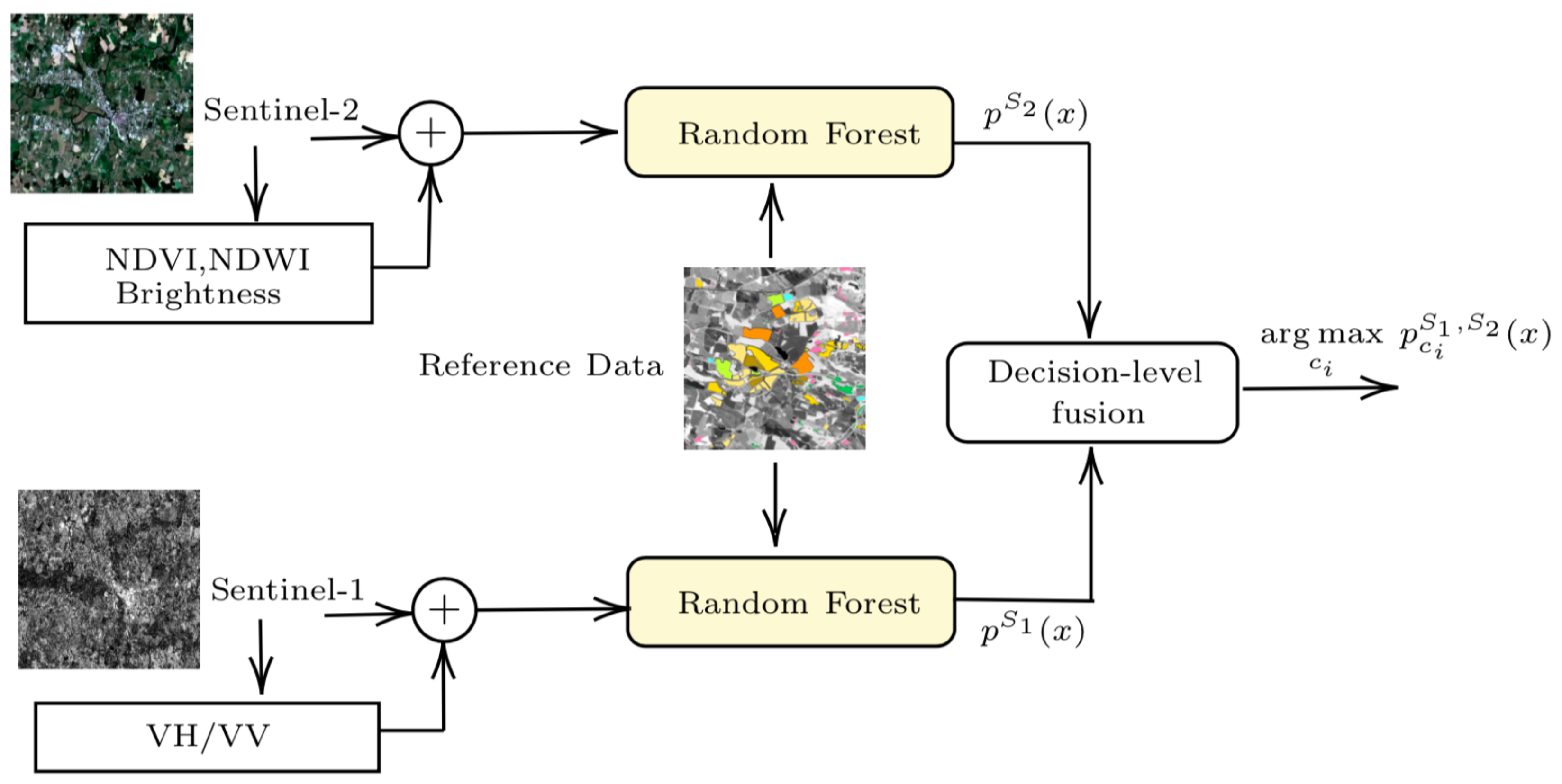
In addition to early fusion, other strategies not applied to high-resolution multitemporal datasets have been proposed in the remote sensing literature to fuse single optical and radar images. For instance, decision-level methods have been proposed to individually classify optical and SAR data and to treat the classifier outputs to yield a final classification decision [59,60,61,62]. Working radar and optical sensors on two different principles allows two complementary classifiers to be trained using two different representations of the input data. Therefore, the combination of two of them will help to improve the classification results obtained by using just one of them. In addition, postdecision classification systems require less training data to overcome the curse of dimensionality issues. Therefore, this work aims to propose a crop mapping processing chain where the synergy of Sentinel’s data is exploited by a decision-level fusion strategy.

3. Methodology

3.1. Random Forest Classifier

Random forest (RF) is a popular ensemble classifier that builds multiple decision trees and merges them to obtain more accurate results [63]. Ensemble prediction uses majority voting to assign a class of unlabeled samples. To construct the ensemble of trees, the concepts of bootstrap aggregating and random selection of features are combined. Both concepts are applied to reduce the correlation between trees, thus creating an expected reduction in the variance of the prediction error. The bootstrap strategy consists of building each tree by a subset of samples (i.e., bootstrapped) that are randomly selected with replacements from the complete training data. Traditionally, two-thirds of samples from the training data set are selected as bootstrapped data.

Each bootstrapped dataset is used to build a single tree by a recursive partitioning algorithm. This iterative algorithm splits the data into two smaller subsets at each node on the tree. At each step, the best split is found by searching through a subset of m features that are randomly selected from the set of all variables. The feature resulting in the largest decrease in impurity is chosen to separate the samples. The grown phase is finished when the terminal nodes or leaves contain very similar samples or when the splitting no longer adds value to the predictions. For implementation purposes, tree building can be stopped when a maximum depth ($maxdepth$) is reached or when the number of samples at the node is below a $minsamples$ threshold. Assuming a classification problem with N different classes and an unlabeled sample x, the ensemble of the predictions in the forest can be used to estimate the posterior class probabilities $p\left(x\right)=\{p_{C_1}\left(x\right),$⋯, and $p_{C_N}\left(x\right)\}$. A natural way is to use the average vote, i.e., calculating the proportion of trees voting for each class [63,64].

3.2. Joint S1-S2 Classification System

By working Sentinel-1 (S1) and Sentinel-2 (S2) on different principles, two complementary, rather than competitive, RF classifiers can be independently trained. The combination of classifiers allows us to reduce the dimensionality of the feature space, which could yield more accurate results. Figure 1 shows how predictions obtained by two independent S1 and S2 classifiers can be combined at the decision-level stage.

In addition to the raw satellite data, some additional features were also included in the optical and radar input data stack. The S1-S2 classification system proposes to apply two independent RF classifiers (reviewed in Section 3.1) on optical and radar data. For each pixel, each classifier i computes its corresponding conditional class probabilities $p^{S_i}\left(x\right)$. Finally, a decision-level fusion strategy was proposed to combine the class probability vectors $p^{S_1}\left(x\right)$ and $p^{S_2}\left(x\right)$. In this work, the following combination rules [65] were studied:

• Product of experts (PoE): Considering $p^{S_1}\left(x\right)$ and $p^{S_2}\left(x\right)$ as individual expert opinions, PoE combines them as a product of experts by multiplying individual probabilities and renormalizing. This can be expressed by:

  $$C_p\left(x\right)=\underset{C_i}{arg\; max}\frac{p_{C_i}^{S_1}\left(x\right)p_{C_i}^{S_2}\left(x\right)}{{\displaystyle \sum _{l=1}^N{p}_{C_i}^{S_1}\left(x\right)p_{C_i}^{S_2}\left(x\right)}};$$

  (1)
• Maximum confidence: The classifier that is most confident in itself gives the predicted class.

  $$C_p\left(x\right)=\underset{C_i}{arg\; max}(p^{S_1}\left(x\right),p^{S_2}\left(x\right));$$

  (2)
• Mean confidence: This combination rule predicts the class reaching the highest average posterior probability value.

  $$C_p\left(x\right)=\underset{C_i}{arg\; max}\frac{1}{2}{\displaystyle \sum _{j=1}^2{p}_{C_i}^{S_j}\left(x\right)};$$

  (3)
• Fusion using the Dempster–Shafer theory: Dempster–Shafer theory can be used to combine multiple classifiers seen as independent information sources. The idea is to consider posterior probability as joint mass values that can be directly used to compute joint beliefs. This strategy assigns the class label for which the belief is maximal.

3.3. SenSAgri Crop Mapping Processing Chain

A binary cropland mask and a crop type map are the two products generated by the SenSAgri processing chain. Figure 2 describes the two-fold methodology, which is mainly based on the supervised S1-S2 classification system of Figure 1. In addition to satellite data, reference data are needed as an input requirement. The level of the land cover and thematic details of the legend must be chosen by the user.

Instead of considering crop mapping as a classification problem with a detailed agricultural legend, the SenSAgri processing chain proposes a specific two-fold strategy. The crop mapping goal is divided into two steps to reduce the influence of the level of details of land cover classes on crop classification results; an example of this is imaging a classification problem where the straw cereals class is divided into very similar wheat and barley classes. As high confusion exists between these two classes, the use of a legend with this high-level detail can lead to incorrect classification results (see Appendix C).

As shown in Figure 2, the first step is the binary detection of the cropland areas. This task is carried out by an S1-S2 classifier system whose training stage considers a legend containing all the land cover classes of the landscape. These results are then used to decide if the pixel can be classified as a crop by the cropland detection strategy described in Section 3.4. This step allowed us to reduce the confusion between agricultural and similar non-crop agricultural land. Finally, the crop type map is obtained by applying a second S1-S2 classifier system on the areas detected by the binary cropland mask. In this case, the reference dataset only contains crop type classes.

3.4. Extraction of Cropland Extent Areas

Given a classification problem of N classes and a pixel x, the ensemble of class probability values obtained by the S1-S2 classification system can be expressed by:

$$\Omega =\{p_{c_i}^{S_1,S_2}\left(x\right)\mid i\in [1\cdots N]\}$$

(4)

Considering the binary cropland detection aim, $\Omega$ can be divided into two subsets, ${\Omega }_{Crop}$ and ${\Omega }_{Non-Crop}$. This split can be easily performed by knowing whether $c_i$ belongs to a crop or a non-crop class. Under this assumption, the probability that a pixel x belongs to a crop class can be denoted as:

$${\displaystyle P_{Crop}\left(x\right)=\sum _{\forall c_i\in {\Omega }_{Crop}}{p}_{c_i}^{S_1,S_2}\left(x\right)}$$

(5)

Thus, the binary cropland mask can be easily obtained by assigning the following to each image pixel x:

$$\left\{\begin{array}{cc}1\hfill & if{P}_{Crop}\left(x\right)>0.5\hfill \\ 0\hfill & \mathrm{otherwise}\hfill \end{array}\right.$$

(6)

4. Study Areas, Satellite Data and Experimental Design

The three European test sites of Figure 3 were studied. The French test site is located in the southwestern France near Toulouse, and the area covers three Sentinel tiles (T30TYP, T31TCJ, T31TCH). Each Sentinel tile covers an extension of 110 × 110 km. The other two test sites cover geographical areas contained on two Sentinel tiles. The Spanish test site is located in the the north of Spain near Valladolid (T30TUL, T30TUM). The Italian test site is located in the south of Italy near Bari (T33TWF, T33TWG). For the French test site, two annual agricultural seasons from October to November were studied. For the rest of the test sites, only one agricultural season was studied. The three test sites involve different crop legends and satellite image coverages.

4.1. Reference Data

Reference data sets describing the study areas were created by considering (i) artificial classes such as buildings, (ii) natural classes such as forests or water bodies and (iii) agricultural classes (see Appendix A). French and Spanish data sets were generated by merging governmental databases and data collected from field campaigns. Reference data were collected during fieldwork campaigns for the Italian test site.

Information from the Land Parcel Information System (LPIS) database was used for agricultural classes for the French and Spanish test sites. For each parcel, this database describes the main cultivated crops according to its farmers’ declarations. The LPIS is obtained under the framework of the Common Agricultural Policy, and it also provides information about temporary/permanent grasslands. Concerning artificial and natural categories, the French National Land Cover database, produced by the French mapping agency (Institut National de l’Information Géographique et Forestière in French), was considered for the French area. A description of governmental databases considered for the Spanish test site can be found in [66]. The resulting reference datasets reflect the spatial heterogeneity of the whole study areas.

4.2. Sentinel-1 Data

Sentinel-1 is an imaging radar mission based on a constellation of two satellites equipped with a C-band SAR sensor. Interferometric Wideswath (IW) mode with VH and VV polarizations and the Level-1 Ground Range detected (GRD) product were used. The spatial resolution was 10 m, and the images were downloaded from the Sentinel Product Exploitation Platform (PEPS). S1tiling processing chain [67] was applied for clipping the Sentinel-1 to the Sentinel-2 tiles. The chain was applied to perform orthorectification and multitemporal filtering to reduce the speckle noise.

Images from ascending and descending orbits acquired at night and day were considered. The French test site was covered by four orbits (8, 30, 110, 132). For this test area, the number of SAR images was equal to 133 and 247 for the 2016 and 2017 agricultural years, respectively. Three orbits (44, 124, 146) were considered for the Italian site, and five orbits (1, 52, 74, 91, 154) were used for the Spanish area. Given the large number of SAR images available from the different orbits, the test sites were covered by a temporal resolution ranging from 12 h up to 3.5 days. To make the irregular temporal sampling resulting from the use of different orbits uniform, images were resampled to a common temporal grid by applying weighted linear interpolation. In addition to the VV and VH polarizations, the VH/VV ratio providing information about vegetation volume was also considered. The incorporation of VH/VV reduces errors associated with the acquisition system or environmental factors (e.g., due to variations in soil moisture). The temporal radar backscatter profiles of the main crop types studied at the French test site are shown in Figure 4.

4.3. Optical Data

Sentinel-2 L2A images and their corresponding cloud masks were obtained from the THEIA web portal. The L2A images were obtained by applying the MAJA (Maccs-Atcor Joint Algorithm) processing chain citeMAJAon Sentinel-2 L1C products. Images were acquired by a single multispectral instrument operating at 13 different spectral bands. In this study, only 10 m and 20 m spatial resolution bands were considered. The 20 m resolution bands were downscaled to 10 meters. Images were resampled to a common temporal grid by applying weighted linear interpolation. This step was necessary (i) to recover missing information resulting from clouds (cloud shadows) and (ii) to uniformly correct the irregular temporal sampling resulting from the use of different Sentinel tiles.

The description of the number of Sentinel-2 acquisitions considered for each test site is described in Appendix B. The number of acquisitions increased in 2017 due to the launch of Sentinel-2B. In addition to the raw optical data, the spectral indices detailed in

Table 1. Optical features computed from Sentinel-2 data.

Spectral Index	Equation
Normalized Difference Vegetation Index	$NDVI=\frac{NIR-R}{NIR+R}$
Normalized Difference Water Index	$NDWI=\frac{G-NIR}{G+NIR}$
Brightness	The norm of the spectral vector

were computed for each studied pixel:

NDVI and NDWI profiles of the main crop types studied at the French test site are shown in Figure 5. The figure shows how winter crops (straw and rapeseed) emerge in winter; they are at full growth in spring, and finally, they are harvested in July.

4.4. Experimental Design

From the reference data sets, training and validation subsets not containing overlapping polygons were generated. The random sampling procedure was used to generate the spatially disjointed training and validation subsets. This split was carried out in ten random trials, which allowed us to statistically evaluate the results with $95\%$ confidence intervals. For the different test sites, a complete description of the reference data set is found in Appendix A. For the different experiments, balanced training sample datasets are created by randomly selecting 2000 samples per class from training polygons. In contrast, imbalanced validation data sets are used in all the experiments by considering all the validation polygon samples.

The hyperparameters of the RF classifier were set by considering the results in [32]. The number of trees was set to 100, and the maximum depth of the tree and the minimum sample leaf size were set to 25. The number of randomly selected features considered for a split in each tree node was set to $\sqrt{p}$, where p is the number of input variables. In addition, all the experiments consider 3 radar and 13 optical features (see Table 1) for the different image acquisitions.

Different evaluation measures were used to evaluate the classification performances. The overall accuracy (OA) was calculated as the total number of correctly-classified pixels divided by the total number of validation pixels, which are described in Appendix A. The F-score for the class was computed as the harmonic mean of the precision and recall and reached its maximum value at 1 and minimum score at 0. The recall was considered as the number of true positives divided by the number of true positives plus the number of false negatives. In contrast, the precision was computed as the number of true positives divided by the number of true positives plus the number of false positives.

The first three experiments were performed to study the complementarity among S2 and S1 classifiers (i.e., whether they were complementary in terms of errors). For these experiments, the 2016 and 2017 agricultural seasons of the French test site were studied. Theoretically, prediction accuracies must improve if both classifiers are accurate and diverse. The agreements and disagreements among RF classifiers trained with S1 and S2 time series were studied. Each input data set was composed of all the available preprocessed optical/radar satellite images. For each year, two optical and radar RF classifiers are independently trained and validated using the data described in Appendix A.

The performances of decision-level fusion strategies described in Section 3.2 were tested and compared on the two French data sets (2016 and 2017). For each pixel x, probabilities $p^{S_1}\left(x\right)$ and $p^{S_2}\left(x\right)$ are estimated by counting the fraction of trees in the forest that vote for each class. In addition to the four postdecision strategies, an early fusion approach was also investigated. This classical strategy consists of training the RF classifier with the stack of all the Sentinel’s images. In our case, the resulting 2016 dataset contains 252 radar and 494 optical features. For the 2017 data set, the total number of features was 1400.

The benefit of fusion was studied for the early classification of Sentinel’s data, where the class of the time series was predicted before it was observed in its entirety. Instead of working with an annual time series, this study has evaluated the benefit of Sentinel’s fusion in an online classification scenario. To perform this task, the French agricultural data sets were divided into three different time periods (see Appendix B). The in-season performances of the S1-S2 classification system were then studied. Each time period was classified by using as input data the stack of its past and current Sentinel’s image acquisitions. The following strategies were tested and compared: (i) individual S1 and S2 classifiers, and (ii) the early and (iii) $PoE$ fusion strategies. In-season classification results are evaluated by annual class labels described in Appendix A. This experiment also investigates the relationship between the dimension of input data and classification results. In addition, some classification results are shown in Appendix E. This last experiment investigates whether increasing the number of training samples could improve the performance of the S12 strategy.

A second family of experiments was performed to extensively evaluate the SenSAgri crop mapping processing chain (Figure 2). Seasonal crop map accuracies are assessed by several experiments during the agricultural year. For this experiment, the $PoE$ fusion strategy was used on the two supervised S1-S2 classification systems. The proposed crop mapping methodology was evaluated on the three European test sites described in Section 4 on three different dates during the agricultural year (Appendix B). Binary crop map results were evaluated and compared with the recent Sen2Agri strategy proposed in the state of the art. The accuracies of crop type maps were also discussed.

5. Results

5.1. Synergy between S1 and S2 Classifiers

The level of agreement between independently trained S1 and S2 classifiers is evaluated here. The obtained results are shown in

Table 2. Classification results obtained by RF classifiers independently trained on Sentinel-1 (S1) and Sentinel-1 (S2) data. F-score values, overall accuracies (OA) and confidence intervals (CI) are computed for the complete French 2016 data set.

France-2016	S1	S2
Wine	87.5	90.8
Straw Cereals	88.5	88.5
Maize	82.9	85.7
Sorghum	31.2	40.7
Soyabeans	58.4	59.5
Sunflowers	86.6	83.0
Alfalfa	52.7	57.3
Grassland	61.7	71.9
Fallow	41.3	49.8
Shrubland	49.8	48.5
Rapeseed	76.3	70.1
Broadleaved Forest	82.1	85.5
Build-up	87.4	89.1
Water	95.6	98.8
Orchard	20.4	38.8
OA	72.6	77.4
CI (${10}^{-2}$)	±0.39	±0.29

and

Table 3. Classification results obtained by RF classifiers independently trained on Sentinel-1 (S1) and Sentinel-1 (S2) data. F-score values, overall accuracies (OA) and confidence intervals (CI) are computed for the complete French 2017 data sets.

France-2017	S1	S2
Orchard	56.0	65.2
Straw Cereal	91.4	89.6
Maize	91.6	94.8
Sorghum	67.2	78.5
Wine	69.4	82.2
Soyabeans	57.8	69.3
Peas	85.5	82.7
Rapeseed	96.2	91.0
Sunflower	92.7	92.0
Temp. grassland	31.7	32.5
Grassland	49.4	63.9
Fallow	30.6	41.8
Schrubland	25.4	31.1
Broadleaved Forest	78.9	88.0
Coniferous Forest	61.7	85.8
Build-up	84.7	89.1
Water	96.8	98.5
Alfafa/clover	39.5	52.2
OA	61.4	70.6
CI (${10}^{-2}$)	±1.16	±0.78

, where values indicate the averaged F-scores obtained by individual classifiers.

It can be observed that both classifiers reach high accuracies for an important number of classes. As expected, the worst accuracies were obtained by classes describing seminatural vegetation areas (fallow, shrubland, temporal grassland or alfalfa). The strong confusion of these herbaceous classes is explained by their similar temporal patterns and their high intraclass variabilities. For instance, perennial fodder crops such as alfalfa and temporal grassland are highly confused.

Comparing the results of Table 2 and Table 3, it can be observed that the highest accuracies are reached by the S2 classifier for both datasets. In addition, it reaches the narrowest 95% confidence interval. Important differences can be observed for some classes by comparing both classifier results. For instance, the difference between S2 and S1 F-score values is equal to $24\%$ for coniferous forests in 2017. The important confusion existing between coniferous and broadleaved forests explains the decrease in accuracy. These confusions can be observed by looking at the 2017 confusion matrix shown in Appendix D.

The S1 classifier is also less accurate for orchard results, which is especially remarkable in 2016. In this case, the orchard class is strongly confused with forest and wine classes. The similar tree structure characterizing forests and orchards has important effects on the discrimination of these classes. The accuracy difference between the two years is mainly due to the different numbers of orchard and wine validation samples described in Appendix A.

Comparing winter and summer crop accuracies, some differences are also observed between the optical and radar results. The S1 classifier reaches the highest accuracies for crop winter classes (rapeseed and straw cereals). The radar classifier achieves better discrimination since high scattering diffusion is captured by radar acquisitions due to the structure and volume of rapeseed plants. The accuracy decrease of the S2 classifier is due to the low number of non-cloudy Sentinel-2 images acquired in the winter season.

In contrast, the S2 classifier reached most of the highest accuracies for summer crop classes (sunflower, maize, sorghum and soybean). Only the sunflower class was well recognized by the S1 classifier, which was mainly due to the presence of the spike at the back of the flower. In general, important confusion exists between sorghum and maize for the S1 classifier. Unfortunately, these classes are only different at the beginning and end of their vegetation phenological cycle. As expected, summer crop minority classes (sorghum and soybean) obtained the lowest accuracies, which was especially remarkable in 2016. More information about the confusion observed by both classifiers for both years is detailed in Appendix D.

Comparing the results obtained in both years, it can be observed that the 2017 dataset obtains more accurate results. One possible reason for this accuracy improvement is the high number of Sentinel images acquired in 2017. However, the F-score values cannot be directly compared for both years since the number of validation samples and the class legends are slightly different for both data sets (Appendix A). For instance, a high difference exists between the number of validation samples for the grassland class.

The complementarity of S1 and S2 classifiers (Table 2 and Table 3) is analyzed by studying their agreements and disagreements. For each validation pixel, the classes predicted by S1 and S2 classifiers ($C_p^{S_1}$,$C_p^{S_2}$) are compared with its reference class $C_r$. Five different metrics are computed: (i) the percentage of correctly classified pixels for both classifiers, (ii) the percentage of correctly classified pixels only for the Sentinel-2 classifier, (iii) the percentage of correctly classified pixels only for the Sentinel-1 classifier, (iv) the percentage of incorrectly classified pixels for both classifiers where the predicted label is the same and (v) the percentage of incorrectly classified pixels for both classifiers where the predicted label is different.

Figure 6 shows the obtained metrics. Agreements among S1 and S2 classifiers are observed by the green bars. The yellow and dark red bars show classifier disagreements. In the case of the yellow bars, they illustrate when one of the two classifiers obtains the correct prediction. In contrast, dark red bars show when both classifiers predict different incorrect classes. Finally, light red bars show when the two classifiers made the same incorrect prediction.

Different behaviors are observed on the different land cover classes. Well-classified classes such as straw cereals or water (see Table 2 and Table 3) obtain a high level of agreement. In contrast, important disagreements are reached by classes obtaining low F-score values. As expected, the highest disagreements were reached by seminatural vegetation classes.

The existence of disagreements confirms the complementarity in terms of errors for both classifiers. The results also show the presence of light red bars, which illustrates that both classifiers can fail in the same way. For instance, both classifiers confuse the orchard class with alfalfa and wine classes. Unfortunately, the agreement on the wrong label for both classifiers can lead to incorrect classification results.

The deep analysis of the results also shows that the confusions of both classifiers are different for some classes. For instance, S2 classifier has problems discriminating between maize and sunflower classes, whereas maize is mainly confused with sorghum by the S1 classifier. The confusions of straw cereal and temporal grassland are also different for both classifiers, which are much less important for the S1 classifier. These conclusions are similar for the two years studied.

5.1.1. Comparison of Decision-Level Fusion Strategies

The average F-score results obtained by different fusion strategies are discussed here.

Table 4. Classification results obtained for the French 2016 data set. Independent S1 and S2 classifiers, early fusion (S12) and postdecision-level strategies are evaluated. F-score values, overall accuracies (OA) and confidence intervals (CI) are computed.

France-2016	S1	S2	S12	$\mathit{PoE}$	$\mathit{Max}$	$\mathit{Mean}$	DS
Wine	87.5	90.8	90.3	94.3	89.9	94.0	92.8
Straw Cereals	88.5	88.5	88.9	90.4	89.0	90.1	89.4
Maize	82.9	85.7	83.7	88.2	82.1	87.9	86.9
Sorghum	31.2	40.7	34.1	45.1	35.9	44.7	42.6
Soyabeans	58.4	59.5	58.3	67.4	56.6	67.5	65.5
Sunflowers	86.6	83.0	83.8	87.0	84.5	86.5	85.7
Alfalfa	52.7	57.3	56.1	64.2	56.8	63.6	60.9
Grass	61.7	71.9	68.2	73.6	63.7	73.5	71.9
Fallow	41.3	49.8	48.3	54.6	45.4	54.4	51.9
Shrubland	49.8	48.5	51.2	58.5	43.7	58.4	55.0
Rapeseed	76.3	70.1	74.1	76.5	70.7	75.9	74.6
Broadleaved Forest	82.1	85.5	86.6	88.0	82.9	87.5	86.1
Build-up	87.4	89.1	92.4	96.1	89.3	94.8	92.2
Water	95.6	98.8	98.4	98.3	97.3	98.4	97.8
Orchard	20.4	38.8	28.9	42.5	28.3	43.9	40.3
OA	72.6	77.4	75.9	81.0	73.4	80.8	79.3
CI (${10}^{-2}$)	0.394	0.294	0.95	0.537	0.499	0.426	0.292

and

Table 5. Classification results obtained for the French 2017 data set. Independent S1 and S2 classifiers, early fusion (S12) and postdecision-level strategies are evaluated. F-scores values, overall accuracies (OA) and confidence intervals (CI) are computed.

France-2017	S1	S2	S12	$\mathit{PoE}$	$\mathit{Max}$	$\mathit{Mean}$	DS
Orchard	56.0	65.2	62.4	71.5	72.1	71.0	67.6
Straw Cereal	91.4	89.6	88.8	91.5	92.1	90.9	90.1
Maize	91.6	94.8	93.7	94.7	94.0	94.6	94.4
Sorghum	67.2	78.5	71.8	79.8	71.6	79.8	78.5
Wine	69.4	82.2	81.0	86.5	84.7	82.6	79.6
Soyabeans	57.8	69.3	62.0	69.5	63.8	69.2	67.7
Peas	85.5	82.7	82.2	87.7	84.8	86.3	84.6
Rapeseed	96.2	91.0	94.9	96.3	93.3	96.2	94.6
Sunflower	92.7	92.0	90.9	92.7	92.7	92.5	92.0
Temporary grassland	31.7	32.5	23.4	35.8	25.5	34.9	32.2
Grassland	49.4	63.9	58.6	63.7	58.6	63.8	63.0
Fallow	30.6	41.8	36.9	46.9	32.2	45.6	41.8
Schrubland	25.4	31.1	26.8	33.3	26.9	34.0	33.4
Broadleaved forests	78.9	88.0	86.8	88.3	87.4	88.5	88.3
Coniferous forests	61.7	85.8	83.8	86.8	71.9	85.9	81.6
Build-up	84.7	89.1	90.6	95.8	88.8	94.2	91.1
Water	96.8	98.5	98.3	98.4	97.3	98.3	96.9
Alfafa/clover	39.5	52.2	42.2	56.6	44.1	56.1	52.6
OA	61.4	70.5	67.0	72.0	67.4	71.8	70.6
CI (${10}^{-2}$)	1.16	0.78	1.24	0.43	0.32	0.35	0.26

confirm that postdecision strategies improve the performances obtained by the individual S1 and S2 classifiers. As expected, the classes that are well classified by individual S1 and S2 classifiers have a low fusion benefit. In contrast, high accuracy gain (approximately 10%) can be observed by some classes, such as alfalfa or orchard, in both data sets.

The results show that the accuracy gain of the early fusion strategy (S12) is low. Even the S12 accuracies are lower than S2 for a considerable number of classes, such as grassland, alfalfa and orchards. In addition, the largest confidence interval is obtained by this fusion strategy. The high dimension of the optical-SAR feature stack (i.e., the curse of dimensionality) could explain the low fusion benefit of early fusion. The product rule ($PoE$) strategy obtains the highest accuracies when compared to the other postdecision fusion methods. The class accuracies have been considerably improved by this fusion strategy. The accuracy gain is remarkable for some classes, such as orchards or alfalfa. In fact, the fusion benefit is high for classes having long yellow bars (see Figure 6), which are well classified for at least one classifier. In this situation, postdecision fusion strategies correctly remove the disagreements among the classifiers. The Dempster–Shafter ($DS$) strategy obtains the lowest accuracies. Classes with uncertainty, such as seminatural vegetation, are strongly penalized by $DS$ fusion. The problem is that $DS$ gives priority to classes reaching high confidence values, which are most of the time well classified.

Figure 7 shows a visual evaluation of the results obtained from the 2017 French dataset. Figure 7a shows the reference polygons used for validation. Land cover maps obtained by individual S1 and S2 classifiers are shown in Figure 7b,c. The classification results of $PoE$ are illustrated in Figure 7d. Comparing the resulting maps, some differences are observed.

The three red boxes of Figure 7a highlight the interest of combining both classifier results. In the case of the top left polygon, it is well classified by $PoE$ thanks to the S1 prediction. In contrast, the alfalfa polygon (on the right) is well classified by $PoE$ thanks to the S2 decision. An interesting visual result is also observed by comparing Figure 7b and Figure 7c. The results show that some edges are lost on the land cover map obtained by the S1 classifier. This loss, which is less remarkable in the $PoE$ results (Figure 7d), can be explained by the perceptual quality of the SAR images.

5.1.2. Interest in Fusion for Early Classification

Finally, the benefit of postfusion strategies for in-season land cover mapping is investigated.

Table 6. Classification results obtained in 2016 at the French test site during the early and mid-agricultural seasons. Independent S1 and S2 classifiers, early fusion (S12) and post-decision level strategies are evaluated. F-score values, overall accuracies (OA) and confidence intervals (CI) are computed.

	28-February				28-June
France-2016	S1	S2	S12	PoE	S1	S2	S12	PoE
Wine	77.9	79.2	84.3	88.3	84.9	87.3	88.0	92.3
Straw Cereals	74.9	84.0	83.9	85.6	87.9	88.3	88.5	90.0
Maize	51.7	60.1	59.7	63.9	72.2	75.3	74.0	78.9
Sorghum	8.7	8.9	9.2	11.8	24.6	19.2	22.8	30.6
Soyabeans	16.4	17.6	18.0	20.8	27.9	27.8	27.1	33.0
Sunflowers	43.3	48.9	50.7	52.3	71.7	70.0	73.5	75.9
Alfalfa	41.5	45.0	49.5	52.6	45.9	51.2	53.1	58.9
Grass	53.2	63.5	66.4	67.1	56.3	69.2	67.3	70.3
Fallow	34.1	41.2	46.3	48.5	38.2	48.1	48.1	52.2
Shrubland	42.6	37.3	46.2	52.8	47.1	44.8	51.1	56.3
Rapeseed	50.6	64.2	64.6	69.2	75.8	70.9	73.7	76.1
Broadleaved Forest	73.6	77.6	81.5	84.2	80.8	82.6	84.8	86.8
Build-up	81.4	84.5	87.7	92.9	85.7	88.9	91.4	95.3
Water	93.9	96.6	97.7	97.9	95.6	98.5	98.4	98.3
Orchard	10.9	16.3	20.5	26.6	16.5	32.1	27.9	39.4
OA	57.8	64.5	67.2	70.7	67.3	72.8	72.7	77.0
CI (${10}^{-2}$)	0.636	0.495	0.575	0.458	0.686	0.534	0.867	0.655

and

Table 7. Classification results obtained in 2017 at the French test site during the early and mid-agricultural seasons. Independent S1 and S2 classifiers, early fusion (S12) and postdecision level strategies are evaluated. F-score values, overall accuracies (OA) and confidence intervals (CI) are computed.

	1-March				5-July
France-2017	S1	S2	S12	PoE	S1	S2	S12	PoE
Orchard	37.9	43.9	52.1	58.7	54.1	55.4	56.1	67.9
Straw Cereal	67.9	73.6	73.1	77.2	90.4	89.0	88.5	91.2
Maize	71.3	72.2	73.3	78.2	81.2	81.9	80.9	85.1
Sorghum	15.7	9.1	9.7	13.7	18.0	14.1	11.4	16.2
Wine	58.8	60.0	65.3	72.8	65.2	79.0	78.9	84.4
Soyabeans	6.4	6.5	8.0	9.3	11.8	5.6	6.7	10.0
Peas	22.2	19.1	23.3	25.6	83.6	70.0	77.6	83.1
Rapeseed	42.8	51.1	52.5	62.5	87.3	83.6	88.3	93.9
Sunflower	38.8	55.1	55.2	57.8	69.7	69.8	69.0	73.7
Temp. grassland	27.0	24.9	25.7	29.6	30.2	30.2	26.8	34.1
Grassland	43.6	53.3	54.1	57.6	47.8	60.0	55.3	61.2
Fallow	26.4	30.0	34.2	37.9	29.8	39.6	37.0	44.8
Schrubland	18.8	24.5	27.0	29.6	20.9	28.8	27.0	31.3
Broadleaved Forest	73.9	80.0	81.6	84.6	79.8	85.4	84.9	87.3
Coniferous	54.2	74.5	78.4	83.0	54.6	84.8	82.0	85.1
Build-up	79.5	76.5	85.0	92.9	85.3	85.3	88.9	95.4
Water	90.9	92.9	93.8	95.4	95.6	97.7	97.7	97.9
Alfafa/clover	26.8	29.8	33.0	37.9	36.2	47.9	41.3	53.1
OA	49.3	55.5	57.4	61.5	58.0	65.2	62.9	68.3
CI (${10}^{-2}$)	0.825	0.979	1.185	0.558	0.392	0.976	1.835	0.585

show seasonal classification accuracies. These results can be compared with classification performances obtained at the end of the agricultural seasons (Table 4 and Table 5). As expected, better and more accurate models are obtained by increasing the number of Sentinel acquisitions. In the same direction, confidence intervals decrease throughout the year. The lowest values are reached at the end of the season. As in the previous experiments, the 2017 dataset obtains more accurate results. The low accuracies of the summer crop classes (soybean or sorghum) in the early season are explained by the fact that crops start growing at the beginning of July (i.e., summer crop plots were all in bare soil in February).

The results show that the gain obtained by fusion strategies is most significant in the early season. The greatest benefits of fusion are obtained when the number of optical images of the time series is low. This confirms previous studies [51] highlighting the interest of incorporating SAR information during the winter period.

Seasonal classification results confirm that the best gain is obtained by the $PoE$ method. The good performance of $PoE$ is remarkable for winter crop classes at the beginning of March. At this time, the F-score of the rapeseed class increases almost $20\%$. Early results show a significant improvement in build-up class for both years. The presence of trees in some validation build-up reference polygons has some impact on the S1 classifier early results, which confuses build-up and orchards. As this confusion does not exist for the S2 classifier, the $PoE$ exploits this information to improve the results.

As previously observed, the early fusion S12 strategy cannot fully benefit from the complementarity of optical and radar information. Although the curse of dimensionality is less important in the early and middle seasons (by reducing the input optical-SAR feature stack size), the F-score difference between $PoE$ and S12 is still important for some classes. F-score values obtained on the rapessed and maize classes in the early season are two clear examples. In addition, a wider confidence interval of S12 means greater uncertainty predictions. Even if there is a significant accuracy difference between S12 and $PoE$, it must be noted that the difference is less remarkable in the early season. The reduction in the number of input features, which has significantly decreased by using fewer images, could explain this result.

5.2. Validation of the Seasonal Crop Map Products

5.2.1. Validation of Seasonal Binary Crop Masks

Precision and recall evaluation metrics are used to assess the quality of seasonal binary cropland maps. These measures are computed on three different dates of the agricultural year. For each studied period, all the available Sentinel images from the starting season are used in the classification process.

Table 8. Binary cropland mask results: average recall and precision metrics over 10 runs. The results obtained from the French test site for the different years are reported on tables Fr-2016 and Fr-2017. The other two tables show the results obtained from the Spanish and Italian data sets.

Fr-2016	Recall			Precision
Class	28-February	28-June	14-October	28-February	28-June	14-October
Non-Crop	97.80	98.69	99.04	95.15	96.04	96.63
Crop	89.06	91.07	92.34	94.84	96.92	97.74
Fr-2017	Recall			Precision
Class	1-March	5-July	2-November	1-March	5-July	2-November
Non-Crop	99.18	99.58	99.69	97.34	97.66	97.65
Crop	90.28	91.47	91.49	96.86	98.39	98.80
Spain	Recall			Precision
Class	4-March	3-July	6-November	4-March	3-July	6-November
Non-Crop	73.07	83.05	84.06	75.10	86.02	88.02
Crop	93.01	96.06	96.62	92.27	95.10	95.34
Italy	Recall			Precision
Class	2-March	1-July	3-November	2-March	1-July	3-November
Non-Crop	78.32	89.36	89.70	85.13	93.90	92.64
Crop	95.26	98.07	97.69	92.66	96.54	96.70

reports crop mask averaged metrics computed over the ten random trials for the different test sites.

The results show that highly accurate binary maps can be obtained for all the test sites. As expected, precision and recall measures improve when the number of satellite acquisitions increases throughout the year. Although the most accurate results were obtained at the end of the agricultural season, the majority of cropland areas were well detected in early summer. The low accuracy of the early season is explained by the absence of summer crops during the winter period.

The most accurate precision values are reached by crop class. In general, crop samples are rarely incorrectly labeled, and the obtained binary masks contain most of the cropland surfaces. Some differences are observed when comparing the French results with the other results. The difference between the different test sites can be explained by the unbalanced number of crop/non-crop reference samples.

Similar and satisfactory results are obtained in the two French agricultural seasons. There is only a slight accuracy difference, which can be explained by the higher number of images acquired during 2017. The French test site obtains high precision but low recall measures for the crop class. Low recall is obtained because some vegetation samples belonging to classes such as grassland and alfalfa are classified as crops. Unfortunately, these errors increase the false positive rate of the crop class. This limitation is less pronounced in the Spanish and Italian datasets, which contain fewer non-crop vegetation samples. In fact, Spanish and Italian reference data sets are mainly composed of crop polygons.

The performances of the binary cropland strategy proposed in Section 3.4 is compared with the Sen2Agri methodology described in [44]. As the S2Agri method only considers Sentinel-2 data, the experiment here is performed by only using optical data. The evaluation is only performed on the 2017 agricultural season of the French test site. The results obtained by the SenSAgri cropland detection strategy can be compared with the Sen2Agri results by looking at

Table 9. Precision and recall measures obtained by SenSagri and Sen2Agri methodologies on the 2017 French data set. The binary detection of cropland areas is performed only by using optical data.

France 2017	Precision			Recall
Crops	1-March	5-July	2-November	1-March	5-July	2-November
SenSAgri	90.28	91.47	91.49	96.86	98.39	98.80
Sen2Agri	84.59	87.39	87.67	91.86	92.25	95.97
France 2017	Precision			Recall
Non crops	1-March	5-July	2-November	1-March	5-July	2-November
SenSAgri	99.18	99.58	99.69	97.34	97.66	97.65
Sen2Agri	97.88	98.76	98.94	95.72	96.49	96.55

.

As expected, the results of Table 9 are lower than Table 8 since radar information is not considered in this experiment. Comparing the Sen2AGri and SenSAgri results, it can be noticed that the proposed SenSAgri strategy considerably improves the classification accuracies. A visual evaluation of the Sen2AGri and SenSAgri results is shown in Figure 8. This last figure illustrates the important accuracy gain of the SenSAgri strategy.

5.2.2. Validation of Seasonal Crop Type Maps

The accuracies of crop type maps generated by the SenSAgri processing chain are assessed here. For the experiment, the cropland areas detected in Section 5.2.1 are classified by an S1-S2 classification system trained with a crop class legend. The $PoE$ fusion strategy is also considered to merge optical and radar classifier decisions. The same reference samples (training and validation), RF hyperparameters and input satellite data of Section 5.2.1 are used. Validation samples belonging to non-crop classes are merged into a single class. Overall accuracies, F-score measures and confidence intervals are computed on three dates of the year.

Table 10. Seasonal crop type map accuracies obtained from the French 2016 test site. F-score values, overall accuracies and confidence intervals are computed over 10 runs.

France-2016	28-February	28-June	14-October
Winter crops
Straw cereals	85.82	90.26	90.57
Raspseed	69.48	76.87	77.39
Summer crops
Maize	63.70	78.91	88.27
Sorghum	10.97	30.70	45.64
Soybean	21.07	33.01	67.45
Sunflower	51.98	76.02	87.08
Non-Crop	94.98	96.25	96.75
OA	85.46	90.30	92.89
CI	0.24	0.22	0.20

,

Table 11. Seasonal crop type map accuracies obtained from the French 2017 test site. F-score values, overall accuracies and confidence intervals are computed over 10 runs.

France-2017	1-March	5-July	2-November
Winter Crops
Straw Cereal	83.66	91.12	91.38
Rapeseed	76.91	96.09	96.22
Peas	37.47	87.98	89.27
Summer Crops
Maize	79.23	93.00	94.44
Sorghum	15.71	68.90	78.98
Soya beans	9.85	37.11	68.49
Sunflower	69.11	91.33	92.85
Non-Crop	98.25	98.61	98.66
OA	93.08	96.81	97.24
CI	0.36	0.24	0.22

,

Table 12. Seasonal crop type map accuracies obtained from the Spanish test site. F-score values, overall accuracies and confidence intervals are computed over 10 runs.

Spain	4-March	3-July	6-November
Winter crops
Cereals	82.98	89.46	90.48
Rapeseed	48.98	73.01	73.56
Summer crops
Maize	50.52	79.41	90.96
Vetch	38.24	48.60	52.04
Grain leguminous	41.84	63.09	65.08
Beet	24.67	76.70	91.67
Potatoes	30.52	73.53	78.15
Sunflower	59.37	79.78	86.36
NoCrop	74.04	84.49	85.97
OA	72.71	83.51	85.51
CI	0.39	0.34	0.31

and

Table 13. Seasonal crop type map accuracies obtained from the Italian test site. F-score values, overall accuracies and confidence intervals are computed over 10 runs.

Italy	2-March	30-June	3-November
Winter crops
Straw cereal	87.38	93.90	94.15
Oat	55.96	64.56	62.77
Leguminous
Horse bean	45.07	71.84	71.16
Chickpea	61.29	84.44	82.41
Vegetables
Asperagus	51.13	59.87	57.30
Brocoli	29.19	44.90	50.69
NoCrop	81.53	91.58	91.13
OA	79.12	89.28	89.11
CI	0.96	0.55	0.58

report the classification results, which demonstrate the capabilities of the SenSAgri chain to map crops over large areas. The resulting overall accuracies are greater than 80% on the different dates for all the test sites. The highest accuracies are obtained for the French test site for both years studied. The results prove the satisfactory identification of major crop types at the early beginning of summer seasons. As expected, accuracies increase throughout the year, and low F-score values are obtained for summer crop classes in March. The results also show that minority classes reach the lowest accuracies. This is the case for sorghum and soybean classes at the French test site. The effect of unbalanced validation sorghum data was more significant in 2016. This explains why different results are obtained for the two French seasons studied. The problem of minority classes is also observed in vegetable classes for the Italian test site.

Crop accuracies reported on Table 10 and Table 11 can be compared with the results obtained in Section 5.1.1 and Section 5.1.2, where crop identification is considered a classical land cover classification problem. The results in Table 10 and Table 11 prove the benefit of removing non-crop areas before the identification of crop types. The gain is particularly noticeable in the early season classification results obtained from the 2017 French dataset (see Table 7). For instance, F-score values obtained by the sunflower class increase more than 10% in the early season. This is explained by the fact that most of the alfalfa and grassland samples are removed by the binary cropland mask. The accuracy gain of the SenSAgri results is less noticeable for the 2016 French dataset, which has fewer non-crop vegetation samples.

Spanish and Italian results show low accuracies for some specific crop classes, including the cases of vetch for Spain and leguminous vegetables for Italy. Some of these classes are poorly represented in the areas of study, which explains their low accuracies. For the Italian test site, only a few reference polygons are available for the broccoli or asparagus classes.

A visual evaluation of the results obtained at the end of the 2017 French agricultural season is shown in Figure 9. The reference polygons describing the validation data set are shown in Figure 9a. The color legend used in Figure 7 is considered.

Figure 9a shows the crop type map obtained by applying a parcel-based majority voting regularization on the SenSAgri pixel-level results. To perform it, polygon boundaries defined by the French Land Parcel Information System (LPIS) database are used. Figure 9 assesses the satisfactory performances of the proposed SenSAgri methodology. Only a few polygons disappear on the left of the image. Unfortunately, some missing crop parcels are not well identified in the binary crop mask because they are classified as no crop polygons. The problem of minority classes can also be observed in Figure 9b (some red polygons belonging to sorghum are not correctly classified). Note that the regularization task used here is only a possible solution to reduce the classification pixel-level noise observed in Figure 7.

6. Discussion

6.1. Joint Exploitation of Sentinel’s Data

The research presented here has confirmed the interest of using joint multitemporal optical and SAR data for early crop mapping. The first experiments assessed the performances and complementarity of independent RF classifiers trained on Sentinel’s data. Comparing the individual results, it has been observed that more accurate land cover maps are derived from Sentinel-2 images. A loss of accuracy up to 5% was obtained by models trained on the Sentinel-1 time series. In addition, optical results have achieved better performances in terms of fine detail preservation.

The results show that RF classifiers trained on optical and SAR data obtain different confusions and predictions. Independent errors were observed by the analysis of the posterior probabilities obtained by each classifier. The complementarity has been especially noticeable for complex land cover classification classes such as grassland, fallows or orchards. To exploit this synergy, an S1-S2 classifier system based on a postdecision fusion strategy has been proposed and evaluated.

Postdecision fusion results have proven that the combination of classifier strengths leads to more accurate predictions. The obtained results have highlighted the limitations of the early fusion strategy, which is the most commonly used method for classifying multimodal time series. The early fusion scheme has learned less accurate models because of the huge dimensional dataset resulting from stacking Sentinel’s optical and SAR images. For this fusion strategy, the empty space phenomenon and the curse of dimensionality have complicated the extraction of useful information. The low performances of early fusion have been confirmed by several experiments performed with different numbers of training samples and satellite images. The results have also shown that early fusion accuracies considerably decrease by reducing the number of training samples. As early fusion models are trained with more image features, this strategy needs much more training data to avoid the Hughes phenomenon. As the availability of reference data can be scarce, it confirms that early fusion is not the most appropriate strategy for large-scale crop mapping.

Among the probabilistic fusion strategies, product of experts (PoE) has achieved the best performance over all combination rules. The product rule solved classifier disagreements by systematically removing confusions appearing in French agricultural seasons. The fusion benefit has been mainly observed in the early season, where averaged overall accuracies have risen more than 6%. This gain has confirmed that the incorporation of SAR data into the joint classifier system can handle the lack of optical images due to winter cloud coverage.

Despite the satisfactory performances of $PoE$, more efforts could be conducted to increase the performances of the classifier fusion system. For instance, information about the class accuracies reached by the individual optical and radar classifiers could be incorporated in the fusion process. Specific rules could also be proposed to exploit when both classifiers provide incorrect and very uncertain predictions. The combination of the RF probabilistic outputs by using a high-level classifier may be another possible fusion strategy to improve the results. Middle fusion strategies could also be investigated to address the high dimensionality of Sentinel’s data. The exploration of dimensionality reduction techniques to extract useful features from Sentinel will be an interesting research field to propose intermediate fusion strategies.

6.2. Seasonal Crop Maps

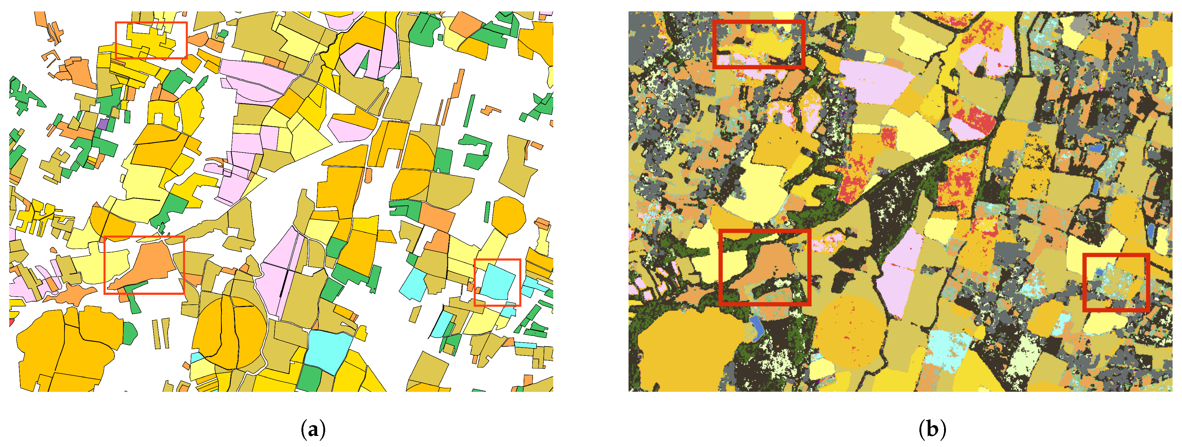
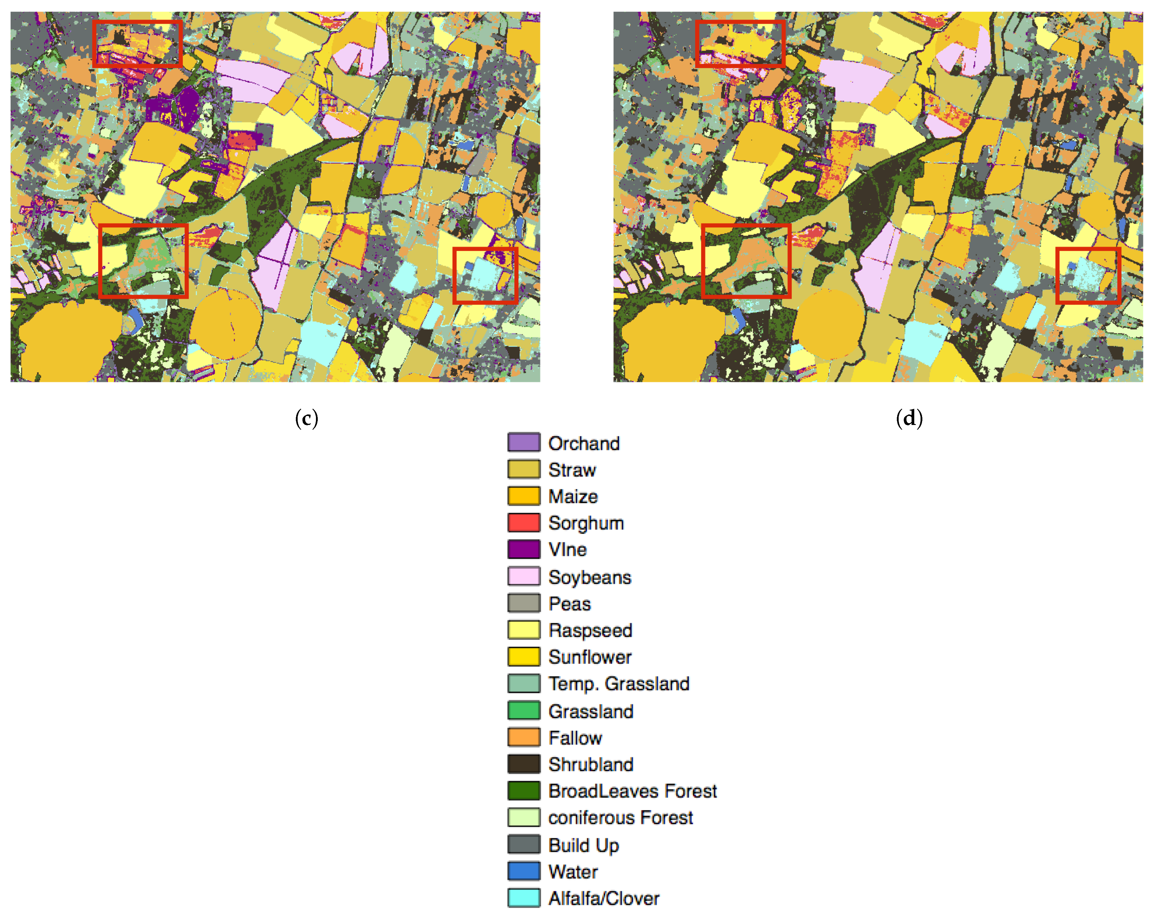
Accurate binary cropland masks and crop type maps were obtained by the proposed SenSAgri methodology. These results have been assessed over large validation data sets covering different geographical areas. The classification performances were evaluated in the early, middle and end of different annual agricultural seasons. The results show that classification accuracies rise throughout the year when the number of image features increases. The best results were reached at the end of the season, where crop phenological cycles were well captured by satellite data. The results confirmed that accurate crop map products can be delivered early (middle of July) during the summer crop growing season.

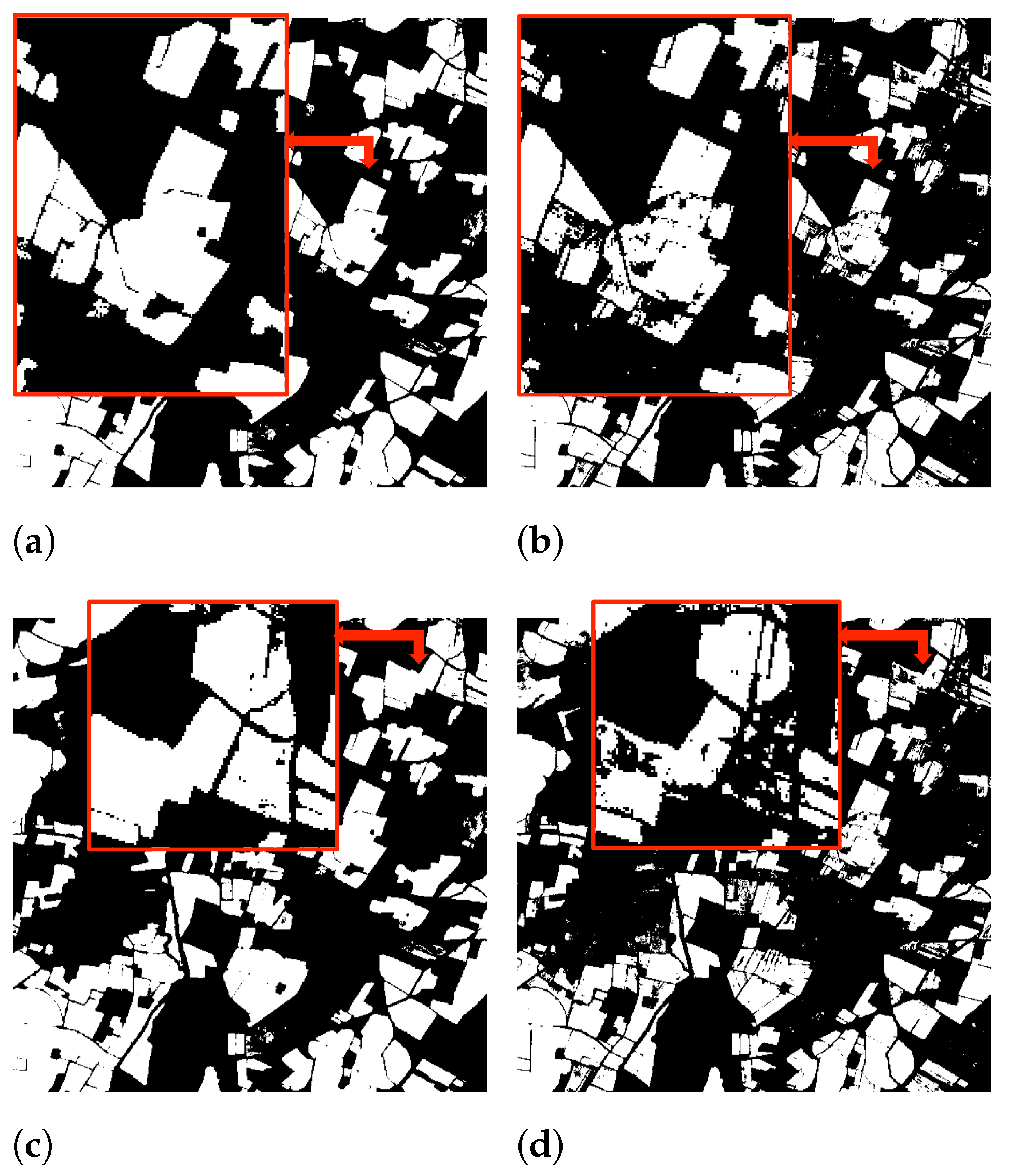
Cropland areas have been correctly identified by binary masks, whose precision and recall values were higher than 90%. The different European test sites obtained similar and satisfactory performances. Binary classification results have shown that crops were rarely confused with non-crop classes. Most of the errors were found in vegetation classes such as alfalfa, fallows or temporary grassland. These classes have not been considered here as cropland areas according to the user crop map product specification. The results also show that confusion between crops and surrounding natural/seminatural vegetation classes can reveal important classification challenges. More efforts could be made in the future to improve the classification of natural/seminatural vegetation areas. It must be remarked that most of the existing crop classification studies have not considered seminatural vegetation classes in their reduced validation datasets.

The results have shown how posterior probabilities obtained by independent RF classifiers can be exploited for the binary detection of agricultural areas. For each pixel, the proposed approach allowed us to estimate the joint probability of belonging to the crop class. The obtained maps recognized cropland areas incorrectly categorized by a classical classification strategy using a complete class legend. The resulting binary cropland masks were compared with those obtained by the Sen2AGri methodology [44], which considers cropland mapping as a binary imbalanced classification problem. Quantitative and visual results have proven that more accurate crop masks are obtained by the SenSAgri methodology. The highest accuracy improvements were achieved by crop class, whose precision and recall measures increased by approximately 5%. In addition, the SenSAgri methodology avoided the definition of the non-crop class data set, which can be challenging given the high variability of non-crop land cover classes describing landscapes. The quality of binary cropland maps could also be improved by optimizing the choice of the binary decision threshold. A strategy to select a threshold depending on an accuracy metric could be proposed.

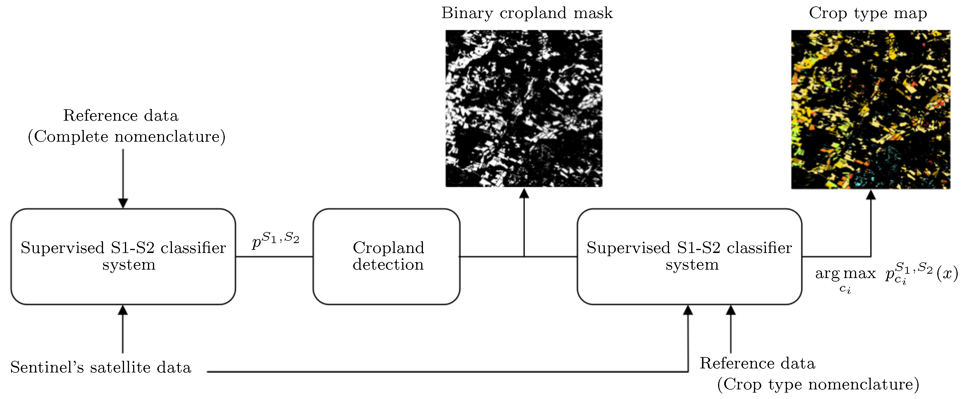
The different experiments have confirmed the interest of detecting cropland areas before classifying the types of crops. The proposed two-fold methodology has reduced the impact of land cover legend definitions on crop classification results. The use of specific classifiers using only crop legends have led to more accurate performances. High-quality crop type maps were obtained with averaged overall accuracies higher than $90\%$. Most of the classes reached satisfactory F-score values, which increased during the season. The lowest F-score values were obtained by minority classes (validation data sets were imbalanced). The different European test sites obtained similar satisfactory results, achieving accurate crop maps at the beginning of the summer season. It must be noted that the early detection of summer crops before the irrigation period could provide essential information to anticipate irrigation water needs.

The quality of crop type maps obtained at the end of the season was also confirmed by a visual evaluation. The results showed how pixel-level classification results can be filtered by a majority vote strategy considering LPIS boundaries. Other filtering strategies could be proposed in the future by considering the classification decisions of the spatial neighborhoods.

Although accurate crop type maps have been produced by the joint use of optical and SAR data, the French test site showed that more accurate maps can be produced by increasing the number of Sentinel-2 images. Accordingly, the incorporation of complementary optical sensors such as Landsat sensors could be investigated to improve the performance of the proposed methodology.

The quality of the resulting crop map products was assessed on large validation datasets, which has rarely been performed in the crop classification literature. Despite the volume of testing data, satisfactory results were obtained with limited training data. Some experiments also confirmed that accuracies could be slightly improved by increasing the number of training samples.

Although the experiments confirmed that the SenSAgri processing chain could be deployed for in-season crop classification, an important consideration needs to be taken into account. The presented results were obtained by in situ data collected from the agricultural season that is to be classified. Consequently, the availability and quality of the in-season reference data have impacted the classification results. Reference data describing non-cropland classes can be obtained from previous years assuming that these classes do not change in consecutive years. In contrast, obtaining crop reference samples describing the agricultural season to be classified can be challenging. According to the recent literature [68,69], one solution could be the exploitation of historical time series and reference data obtained during previous years.

7. Conclusions

In the framework of the H2020 SenSAgri project, this work has proposed a crop mapping processing chain combining both S1 radar and S2 optical data. The proposed two-fold methodology obtained accurate crop map products over three European areas with different cropping systems in the early season. Cropland surfaces and dominant crop types were well recognized in the early, middle and late seasons with limited training data. The results show how postdecision fusion strategies allow the joint exploitation of Sentinel’s time series facing the high dimensionality data challenge. The proposed fusion scheme reduced the amount of training data required by early fusion strategies. Different experiments demonstrated the complementarity of SAR and optical satellite image time series. In particular, the interest in data fusion for early in-season crop mapping has been confirmed. Further experiments will be performed to exploit the several years of Sentinel’s acquisitions. Past reference data sets, Sentinel’s data and crop map predictions will be exploited to improve early in-season crop mapping.

References

1. Whitcraft, A.K.; Becker-Reshef, I.; Killough, B.D.; Justice, C.O. Meeting Earth Observation Requirements for Global Agricultural Monitoring: An Evaluation of the Revisit Capabilities of Current and Planned Moderate Resolution Optical Earth Observing Missions. Remote Sens. 2015, 7, 1482–1503. [Google Scholar] [CrossRef] [Green Version]
2. Whitcraft, A.K.; Becker-Reshef, I.; Justice, C.O. A Framework for Defining Spatially Explicit Earth Observation Requirements for a Global Agricultural Monitoring Initiative (GEOGLAM). Remote Sens. 2015, 7, 1461–1481. [Google Scholar] [CrossRef] [Green Version]
3. Fritz, S.; See, L.; McCallum, I.; You, L.; Bun, A.; Moltchanova, E.; Duerauer, M.; Albrecht, F.; Schill, C.; Perger, C.; et al. Mapping global cropland and field size. Glob. Chang. Biol. 2015, 21, 1980–1992. [Google Scholar] [CrossRef] [PubMed]
4. Ozdogan, M.; Woodcock, C.E. Resolution dependent errors in remote sensing of cultivated areas. Remote Sens. Environ. 2006, 103, 203–217. [Google Scholar] [CrossRef]
5. Friedl, M.; McIver, D.; Hodges, J.; Zhang, X.; Muchoney, D.; Strahler, A.; Woodcock, C.; Gopal, S.; Schneider, A.; Cooper, A.; et al. Global land cover mapping from MODIS: Algorithms and early results. Remote Sens. Environ. 2002, 83, 287–302. [Google Scholar] [CrossRef]
6. Chen, J.; Chen, J.; Liao, A.; Cao, X.; Chen, L.; Chen, X.; He, C.; Han, G.; Peng, S.; Lu, M.; et al. Global land cover mapping at 30 m resolution: A POK-based operational approach. ISPRS J. Photogramm. Remote Sens. 2015, 103, 7–27. [Google Scholar] [CrossRef] [Green Version]
7. Bontemps, S.; Defourny, P.; Bogaert, E.V.; Arino, O.; Kalogirou, V.; Perez, J.R. GLOBCOVER 2009-Products Description and Validation Report; JRC49240; MEDIAS-France: Toulouse, France, 2011. [Google Scholar]
8. Fritz, S.; See, L.; McCallum, I.; Schill, C.; Obersteiner, M.; van der Velde, M.; Boettcher, H.; Havlík, P.; Achard, F. Highlighting continued uncertainty in global land cover maps for the user community. Environ. Res. Lett. 2011, 6, 044005. [Google Scholar] [CrossRef]
9. Pérez-Hoyos, A.; Rembold, F.; Kerdiles, H.; Gallego, J. Comparison of Global Land Cover Datasets for Cropland Monitoring. Remote Sens. 2017, 9, 1118. [Google Scholar] [CrossRef] [Green Version]
10. Waldner, F.; Fritz, S.; Di Gregorio, A.; Defourny, P. Mapping Priorities to Focus Cropland Mapping Activities: Fitness Assessment of Existing Global, Regional and National Cropland Maps. Remote Sens. 2015, 7, 7959–7986. [Google Scholar] [CrossRef] [Green Version]
11. Fritz, S.; See, L.; Bayas, J.C.L.; Waldner, F.; Jacques, D.; Becker-Reshef, I.; Whitcraft, A.; Baruth, B.; Bonifacio, R.; Crutchfield, J.; et al. A comparison of global agricultural monitoring systems and current gaps. Agric. Syst. 2019, 168, 258–272. [Google Scholar] [CrossRef]
12. Gascon, F. Sentinel-2 for Agricultural Monitoring. In Proceedings of the IGARSS 2018—2018 IEEE International Geoscience and Remote Sensing Symposium, Valencia, Spain, 22–27 July 2018; pp. 8166–8168. [Google Scholar] [CrossRef]
13. Veloso, A.; Mermoz, S.; Bouvet, A.; Le Toan, T.; Planells, M.; Dejoux, J.F.; Ceschia, E. Understanding the temporal behavior of crops using Sentinel-1 and Sentinel-2-like data for agricultural applications. Remote Sens. Environ. 2017, 199, 415–426. [Google Scholar] [CrossRef]
14. SenSAgri Projet. Available online: http://sensagri.eu/ (accessed on 15 November 2021).
15. Defourny, P.; Bontemps, S.; Bellemans, N.; Cara, C.; Dedieu, G.; Guzzonato, E.; Hagolle, O.; Inglada, J.; Nicola, L.; Rabaute, T.; et al. Near real-time agriculture monitoring at national scale at parcel resolution: Performance assessment of the Sen2-Agri automated system in various cropping systems around the world. Remote Sens. Environ. 2019, 221, 551–568. [Google Scholar] [CrossRef]
16. Maxwell, A.E.; Warner, T.A.; Fang, F. Implementation of machine-learning classification in remote sensing: An applied review. Int. J. Remote Sens. 2018, 39, 2784–2817. [Google Scholar] [CrossRef] [Green Version]
17. Gómez, C.; White, J.C.; Wulder, M.A. Optical remotely sensed time series data for land cover classification: A review. ISPRS J. Photogramm. Remote Sens. 2016, 116, 55–72. [Google Scholar] [CrossRef] [Green Version]
18. Weiss, M.; Jacob, F.; Duveiller, G. Remote sensing for agricultural applications: A meta-review. Remote Sens. Environ. 2020, 236, 111402. [Google Scholar] [CrossRef]
19. Gumma, M.K.; Nelson, A.; Thenkabail, P.S.; Singh, A.N. Mapping rice areas of South Asia using MODIS multitemporal data. J. Appl. Remote Sens. 2011, 5, 053547. [Google Scholar] [CrossRef] [Green Version]
20. Chang, J.; Hansen, M.C.; Pittman, K.; Carroll, M.; DiMiceli, C. Corn and Soybean Mapping in the United States Using MODIS Time-Series Data Sets. Agron. J. 2007, 99, 1654–1664. [Google Scholar] [CrossRef]
21. Pittman, K.; Hansen, M.C.; Becker-Reshef, I.; Potapov, P.V.; Justice, C.O. Estimating Global Cropland Extent with Multi-year MODIS Data. Remote Sens. 2010, 2, 1844–1863. [Google Scholar] [CrossRef] [Green Version]
22. Wardlow, B.; Egbert, S.; Kastens, J. Analysis of time-series MODIS 250 m vegetation index data for crop classification in the U.S. Central Great Plains. Remote Sens. Environ. 2007, 108, 290–310. [Google Scholar] [CrossRef] [Green Version]
23. Xiong, J.; Thenkabail, P.S.; Gumma, M.K.; Teluguntla, P.; Poehnelt, J.; Congalton, R.G.; Yadav, K.; Thau, D. Automated cropland mapping of continental Africa using Google Earth Engine cloud computing. ISPRS J. Photogramm. Remote Sens. 2017, 126, 225–244. [Google Scholar] [CrossRef] [Green Version]
24. Yu, L.; Wang, J.; Clinton, N.; Xin, Q.; Zhong, L.; Chen, Y.; Gong, P. FROM-GC: 30 m global cropland extent derived through multisource data integration. Int. J. Digit. Earth 2013, 6, 521–533. [Google Scholar] [CrossRef]
25. Johnsan, D.; Mueller, R. The 2009 Cropland Data Layer. Photogramm. Eng. Remote Sens. 2010, 76, 1201–1205. [Google Scholar]
26. Boryan, C.; Yang, Z.; Mueller, R.; Craig, M. Monitoring US agriculture: The US Department of Agriculture, National Agricultural Statistics Service, Cropland Data Layer Program. Geocarto Int. 2011, 26, 341–358. [Google Scholar] [CrossRef]
27. Waldner, F.; Canto, G.S.; Defourny, P. Automated annual cropland mapping using knowledge-based temporal features. ISPRS J. Photogramm. Remote Sens. 2015, 110, 1–13. [Google Scholar] [CrossRef]
28. Biradar, C.M.; Thenkabail, P.S.; Noojipady, P.; Li, Y.; Dheeravath, V.; Turral, H.; Velpuri, M.; Gumma, M.K.; Gangalakunta, O.R.P.; Cai, X.L.; et al. A global map of rainfed cropland areas (GMRCA) at the end of last millennium using remote sensing. Int. J. Appl. Earth Observ. Geoinf. 2009, 11, 114–129. [Google Scholar] [CrossRef]
29. Liu, L.; Xiao, X.; Qin, Y.; Wang, J.; Xu, X.; Hu, Y.; Qiao, Z. Mapping cropping intensity in China using time series Landsat and Sentinel-2 images and Google Earth Engine. Remote Sens. Environ. 2020, 239, 111624. [Google Scholar] [CrossRef]
30. Waldner, F.; Abelleyra, D.D.; Verón, S.R.; Zhang, M.; Wu, B.; Plotnikov, D.; Bartalev, S.; Lavreniuk, M.; Skakun, S.; Kussul, N.; et al. Towards a set of agrosystem-specific cropland mapping methods to address the global cropland diversity. Int. J. Remote Sens. 2016, 37, 3196–3231. [Google Scholar] [CrossRef] [Green Version]
31. Belgiu, M.; Drăguţ, L. Random forest in remote sensing: A review of applications and future directions. ISPRS J. Photogramm. Remote Sens. 2016, 114, 24–31. [Google Scholar] [CrossRef]
32. Pelletier, C.; Valero, S.; Inglada, J.; Champion, N.; Dedieu, G. Assessing the robustness of Random Forests to map land cover with high resolution satellite image time series over large areas. Remote Sens. Environ. 2016, 187, 156–168. [Google Scholar] [CrossRef]
33. Inglada, J.; Vincent, A.; Arias, M.; Tardy, B.; Morin, D.; Rodes, I. Operational High Resolution Land Cover Map Production at the Country Scale Using Satellite Image Time Series. Remote Sens. 2017, 9, 95. [Google Scholar] [CrossRef] [Green Version]
34. Teluguntla, P.; Thenkabail, P.S.; Oliphant, A.; Xiong, J.; Gumma, M.K.; Congalton, R.G.; Yadav, K.; Huete, A. A 30-m landsat-derived cropland extent product of Australia and China using random forest machine learning algorithm on Google Earth Engine cloud computing platform. ISPRS J. Photogramm. Remote Sens. 2018, 144, 325–340. [Google Scholar] [CrossRef]
35. Tatsumi, K.; Yamashiki, Y.; Canales Torres, M.A.; Taipe, C.L.R. Crop classification of upland fields using Random forest of time-series Landsat 7 ETM+ data. Comput. Electron. Agric. 2015, 115, 171–179. [Google Scholar] [CrossRef]
36. Immitzer, M.; Vuolo, F.; Atzberger, C. First Experience with Sentinel-2 Data for Crop and Tree Species Classifications in Central Europe. Remote Sens. 2016, 8, 166. [Google Scholar] [CrossRef]
37. Belgiu, M.; Csillik, O. Sentinel-2 cropland mapping using pixel-based and object-based time-weighted dynamic time warping analysis. Remote Sens. Environ. 2018, 204, 509–523. [Google Scholar] [CrossRef]
38. Zhong, L.; Hu, L.; Zhou, H. Deep learning based multi-temporal crop classification. Remote Sens. Environ. 2019, 221, 430–443. [Google Scholar] [CrossRef]
39. Rußwurm, M.; Körner, M. Temporal Vegetation Modelling Using Long Short-Term Memory Networks for Crop Identification from Medium-Resolution Multi-spectral Satellite Images. In Proceedings of the 2017 IEEE Conference on Computer Vision and Pattern Recognition Workshops (CVPRW), Salt Lake City, UT, USA, 18–22 June 2018; pp. 1496–1504. [Google Scholar]
40. Rußwurm, M.; Körner, M. Self-attention for raw optical Satellite Time Series Classification. ISPRS J. Photogramm. Remote Sens. 2020, 169, 421–435. [Google Scholar] [CrossRef]
41. Ji, S.; Zhang, C.; Xu, A.; Shi, Y.; Duan, Y. 3D Convolutional Neural Networks for Crop Classification with Multi-Temporal Remote Sensing Images. Remote Sens. 2018, 10, 75. [Google Scholar] [CrossRef] [Green Version]
42. Stoian, A.; Poulain, V.; Inglada, J.; Poughon, V.; Derksen, D. Land Cover Maps Production with High Resolution Satellite Image Time Series and Convolutional Neural Networks: Adaptations and Limits for Operational Systems. Remote Sens. 2019, 11, 1986. [Google Scholar] [CrossRef] [Green Version]
43. Inglada, J.; Arias, M.; Tardy, B.; Hagolle, O.; Valero, S.; Morin, D.; Dedieu, G.; Sepulcre, G.; Bontemps, S.; Defourny, P.; et al. Assessment of an Operational System for Crop Type Map Production Using High Temporal and Spatial Resolution Satellite Optical Imagery. Remote Sens. 2015, 7, 12356–12379. [Google Scholar] [CrossRef] [Green Version]
44. Valero, S.; Morin, D.; Inglada, J.; Sepulcre, G.; Arias, M.; Hagolle, O.; Dedieu, G.; Bontemps, S.; Defourny, P.; Koetz, B. Production of a Dynamic Cropland Mask by Processing Remote Sensing Image Series at High Temporal and Spatial Resolutions. Remote Sens. 2016, 8, 55. [Google Scholar] [CrossRef] [Green Version]
45. Pierce, L.E.; Bergen, K.M.; Dobson, M.; Ulaby, F.T. Multitemporal Land-Cover Classification Using SIR-C/X-SAR Imagery. Remote Sens. Environ. 1998, 64, 20–33. [Google Scholar] [CrossRef]
46. Engdahl, M.E.; Hyyppa, J.M. Land-cover classification using multitemporal ERS-1/2 InSAR data. IEEE Trans. Geosci. Remote Sens. 2003, 41, 1620–1628. [Google Scholar] [CrossRef]
47. Robertson, L.D.; Davidson, A.M.; McNairn, H.; Hosseini, M.; Mitchell, S.; de Abelleyra, D.; Verón, S.; le Maire, G.; Plannells, M.; Valero, S.; et al. C-band synthetic aperture radar (SAR) imagery for the classification of diverse cropping systems. Int. J. Remote Sens. 2020, 41, 9628–9649. [Google Scholar] [CrossRef]
48. Joshi, N.; Baumann, M.; Ehammer, A.; Fensholt, R.; Grogan, K.; Hostert, P.; Jepsen, M.R.; Kuemmerle, T.; Meyfroidt, P.; Mitchard, E.T.A.; et al. A Review of the Application of Optical and Radar Remote Sensing Data Fusion to Land Use Mapping and Monitoring. Remote Sens. 2016, 8, 70. [Google Scholar] [CrossRef] [Green Version]
49. Amarsaikhan, D.; Douglas, T. Data fusion and multisource image classification. Int. J. Remote Sens. 2004, 25, 3529–3539. [Google Scholar] [CrossRef]
50. Chang, N.B.; Bai, K. Multisensor Data Fusion and Machine Learning for Environmental Remote Sensing; ImprintCRC Press: Boca Raton, FL, USA, 2018; pp. 1–508. [Google Scholar] [CrossRef]
51. Inglada, J.; Vincent, A.; Arias, M.; Marais-Sicre, C. Improved Early Crop Type Identification By Joint Use of High Temporal Resolution SAR And Optical Image Time Series. Remote Sens. 2016, 8, 362. [Google Scholar] [CrossRef] [Green Version]
52. Steinhausen, M.J.; Wagner, P.D.; Narasimhan, B.; Waske, B. Combining Sentinel-1 and Sentinel-2 data for improved land use and land cover mapping of monsoon regions. Int. J. Appl. Earth Observ. Geoinf. 2018, 73, 595–604. [Google Scholar] [CrossRef]
53. Clerici, N.; Calderón, C.A.V.; Posada, J.M. Fusion of Sentinel-1A and Sentinel-2A data for land cover mapping: A case study in the lower Magdalena region, Colombia. J. Maps 2017, 13, 718–726. [Google Scholar] [CrossRef] [Green Version]
54. Ienco, D.; Interdonato, R.; Gaetano, R.; Ho Tong Minh, D. Combining Sentinel-1 and Sentinel-2 Satellite Image Time Series for land cover mapping via a multi-source deep learning architecture. ISPRS J. Photogramm. Remote Sens. 2019, 158, 11–22. [Google Scholar] [CrossRef]
55. Kussul, N.; Lavreniuk, M.; Skakun, S.; Shelestov, A. Deep Learning Classification of Land Cover and Crop Types Using Remote Sensing Data. IEEE Geosci. Remote Sens. Lett. 2017, 14, 778–782. [Google Scholar] [CrossRef]
56. Van Tricht, K.; Gobin, A.; Gilliams, S.; Piccard, I. Synergistic Use of Radar Sentinel-1 and Optical Sentinel-2 Imagery for Crop Mapping: A Case Study for Belgium. Remote Sens. 2018, 10, 1642. [Google Scholar] [CrossRef] [Green Version]
57. Pacifici, F.; Frate, F.D.; Emery, W.J.; Gamba, P.; Chanussot, J. Urban Mapping Using Coarse SAR and Optical Data: Outcome of the 2007 GRSS Data Fusion Contest. IEEE Geosci. Remote Sens. Lett. 2008, 5, 331–335. [Google Scholar] [CrossRef] [Green Version]
58. Pal, M.; Foody, G. Feature Selection for Classification of Hyperspectral Data by SVM. IEEE Trans. Geosci. Remote Sens. 2010, 48, 2297–2307. [Google Scholar] [CrossRef] [Green Version]
59. Zhang, J. Multi-source remote sensing data fusion: Status and trends. Int. J. Image Data Fusion 2010, 1, 5–24. [Google Scholar] [CrossRef] [Green Version]
60. Ban, Y.; Hu, H.; Rangel, I.M. Fusion of Quickbird MS and RADARSAT SAR data for urban land-cover mapping: Object-based and knowledge-based approach. Int. J. Remote Sens. 2010, 31, 1391–1410. [Google Scholar] [CrossRef]
61. Ducrot, D.; Pretus, J.L. Land cover discrimination potential of radar multitemporal series and optical multispectral images in a Mediterranean cultural landscape. Int. J. Remote Sens. 2004, 25, 3513–3528. [Google Scholar]
62. Waske, B.; Benediktsson, J.A. Fusion of Support Vector Machines for Classification of Multisensor Data. IEEE Trans. Geosci. Remote Sens. 2007, 45, 3858–3866. [Google Scholar] [CrossRef]
63. Breiman, L. Random Forests. Mach. Learn. 2001, 45, 5–32. [Google Scholar] [CrossRef] [Green Version]
64. Bostrom, H. Estimating class probabilities in random forests. In Proceedings of the Sixth International Conference on Machine Learning and Applications (ICMLA 2007), Cincinnati, OH, USA, 13–15 December 2007; pp. 211–216. [Google Scholar]
65. Kittler, J.; Hatef, M.; Duin, R.P.W.; Matas, J. On combining classifiers. IEEE Trans. Pattern Anal. Mach. Intell. 1998, 20, 226–239. [Google Scholar] [CrossRef] [Green Version]
66. Paredes Gómez, V.; Medina, V.; Bengoa, J.; Nafría, D. Accuracy Assessment of a 122 Classes Land Cover Map Based on Sentinel-2, Landsat 8 and Deimos-1 Images and Ancillary Data. In Proceedings of the IGARSS 2018-2018 IEEE International Geoscience and Remote Sensing Symposium, Valencia, Spain, 22–27 July 2018; pp. 5453–5456. [Google Scholar] [CrossRef]
67. Koleck, T.; Ballere, M.A. S1Tiling, A multi-purpose Open Source Processing Chain for 704 Sentinel-1 Tim Series. In Proceedings of the ESA, Living Planet Symposium, Milan, Italy, 13–17 May 2019. [Google Scholar]
68. Tardy, B.; Inglada, J.; Michel, J. Assessment of Optimal Transport for Operational Land-Cover Mapping Using High-Resolution Satellite Images Time Series without Reference Data of the Mapping Period. Remote Sens. 2019, 11, 1047. [Google Scholar] [CrossRef] [Green Version]
69. Flamary, R.; Fauvel, M.; Dalla Mura, M.; Valero, S. Analysis of multi-temporal classification techniques for forecasting image times series. Geosci. Remote Sens. Lett. (GRSL) 2015, 12, 953–957. [Google Scholar] [CrossRef]
Figure 1. Supervised S1-S2 classifier system combining the predictions of two independent Sentinel-1 and Sentinel-2 classifiers. The individual class probability distributions obtained by each classifier are fused at the decision-level stage.
Remotesensing 13 04891 g001
Figure 2. Crop mapping processing chain.
Remotesensing 13 04891 g002
Figure 3. Satellite footprints for the three European test sites.
Remotesensing 13 04891 g003
Figure 4. Temporal radar backscatter profiles of the main French crop types. Time series are averaged at parcel level.
Remotesensing 13 04891 g004
Figure 5. Temporal NDVI and NDWI profiles of the main French crop types. Time series are averaged at the parcel level.
Remotesensing 13 04891 g005
Figure 6. The complementarity of both classifiers is analyzed by studying their agreements and disagreements. The classes predicted by S1 ( C p S 1 ) and S2 ( C p S 2 ) classifiers are compared with reference classes ( C r ). (a) Agreements and disagreements obtained from the French 2016 data set. (b) Agreements and disagreements obtained from the French 2017 data set.
Remotesensing 13 04891 g006
Figure 7. Land cover maps obtained at the end of the agricultural season for the French 2017 dataset. The map obtained by the P o E fusion strategy is compared with the maps obtained by the individual S1 and S2 classifiers. The three red boxes of Figure 7a highlight the interest of combining both classifier results. (a) Reference polygons. (b) S1 classifier. (c) S2 classifier. (d) P o E .
Remotesensing 13 04891 g007aRemotesensing 13 04891 g007b
Figure 8. Comparison between binary crop mask products obtained by only using optical data for the 2017 French agricultural season. Figure 8a,c shows crop masks obtained by the proposed SenSAgri method. Figure 8b,d show crop masks obtained by the Sen2Agri processing chain. (a) SenSAgri crop mask. (b) Sen2Agri crop mask. (c) SenSAgri crop mask. (d) Sen2Agri crop mask.
Remotesensing 13 04891 g008
Figure 9. Land cover maps obtained at the end of the agricultural season for the French 2017 dataset. The same legend used in Figure 7 is considered. (a) Reference polygons. (b) SenSAgri crop map product.
Remotesensing 13 04891 g009