Characterizing Rain Cells as Measured by a Ka-Band Nadir Radar Altimeter: First Results and Impact on Future Altimetry Missions

Abstract

The impact of large atmospheric attenuation events on data quality and availability is a critical aspect for future altimetry missions based on Ka-band altimetry. The SARAL/AltiKa mission and its Ka-band nadir altimeter offer a unique opportunity to assess this impact. Previous publications (Tournadre et al., 2009, 2015) already analyzed the impact of rain on the waveforms at Ka-band and proposed a definition of an elaborate rain flag. This notion tends to give a simpler black and white view of the atmospheric attenuation when the effect on the altimeter measurement is intense. However, in practice, there is a continuum of measurements that may be partially distorted or corrupted by rain events. The present study proposes a wider point of view, directly using the timeseries of the Ka-band altimeter backscattering coefficient for the first time, when previous studies relied on microwave radiometer (MWR) observations or model analyses with coarser resolutions. As guidelines for future Ka-band missions concerning the impact of the atmosphere, the Attenuation CElls Characterization ALgorithm (ACECAL) approach not only provides more representative statistics on rain cells (occurrences, amplitude, size), but also describes the internal structure of the cells. The actual atmospheric attenuation retrieved with ACECAL is about four times larger than the attenuation retrieved from the MWR. At a global scale, 1% of the measurements are affected by an attenuation larger than 23 dB and 10% of the atmospheric attenuation events have a size larger than 40 km. At regional scale, some areas of particular interest for oceanography as Gulf Stream, North Pacific and Brazil currents are more systematically affected compared with global statistics, with atmospheric attenuation up to 8 dB and cell size larger than 25 km when rain occurs. This study also opens some perspectives on the benefits that the community could be drawn from the systematic distribution of the rain cells parameters as secondary products of altimetry missions.

1. Precipitation and Atmospheric Attenuation in the Context of Altimetry Missions

Satellite altimetry missions measure the sea surface height (SSH) at a global scale and with increasing accuracy since 1992 [1]. The altimeter signal is traditionally emitted in the Ku band at around 13.5 GHz as used by Topex (13.6 GHz) and Poseidon (13.65 GHz) altimeters [2] up to the latest Jason-3 (13.6 GHz) and Sentinel-3 (13.575 GHz) series [3].

The attenuation of microwave radar pulse depends on the moist air refractivity index, characterized by the pressure, the temperature, the water vapor, the cloud liquid water content and the rain rate. When the attenuation is too large, the shape of the waveform measured by a classical nadir altimeter is too far from the theoretical Brown model, and the retracking algorithm fails to estimate the geophysical parameters: the range, the surface wave height (SWH), the backscattering coefficient (${\sigma }_0$) from which the wind speed is computed, and the slope of the trailing edge related to the altimeter mispointing angle. However, even with lower distortions, the error on these parameters could be unacceptable with respect to the budget error.

Atmospheric attenuation ($\Delta {\sigma }_0$) at the Ku band has been specifically characterized since the very beginning of the spatial altimetry era. As the Ku band is mostly affected by rain, early papers [4,5] are dedicated to characterizing the impact of rain on the Topex/Poseidon observations. Rain flag and even rain rate are estimated from the difference between altimeter backscattering coefficients at the main Ku band and the secondary C band. Later on, the parameterization of the Ku/C ${\sigma }_0$ relation is updated for Jason-1 and the Ku/S ${\sigma }_0$ relation for Envisat [6,7]. Validation against Tropical Rainfall Measuring Mission (TRMM) observations showed better performances using the Tournadre relation [8]. The different studies agree on a proportion of measurements affected by rain of between 1% and 5% of the total number of observations of the ocean.

The CNES/ISRO SARAL/AltiKa mission which launched in 2013 was the first attempt by an altimetry mission to use a central frequency in the Ka band at 35.75 GHz. Using a higher frequency allowed the footprint of the altimeter to reduce from 15 km at the Ku band to 4 km, but also the range noise and the impact of the ionosphere [9]. Since 2013, this mission has proven the benefits of measurements at the Ka band to oceanography, even extending the boundaries of altimetry to new scientific fields (coastal oceanography, cryospheric sciences, hydrology) [10,11]. The major counterpart in terms of SSH monitoring is a larger sensitivity to the water in the atmosphere: the altimeter backscattering coefficient atmospheric attenuation is seven times larger at the Ka band than at the Ku band [12]. Before the launch of SARAL/AltiKa mission, the expected impact of rain onto altimeter waveform and the foreseen percentage of non-valid data have been studied, and an innovative algorithm to flag the data has been developed in two successive papers by Tournadre et al. [13,14]. The authors analyzed the effect of cells onto altimeter measurement using empirical relation for attenuation and simulated waveforms. The amplitude of the rain events but also the variability over the altimeter footprint size both have an impact. The validation performed over actual measurements [15] has shown the good performance of the so-called Matching Pursuit (MP) flagging algorithm and better availability of the observations than expected in the pre-flight study [13] due to a particularly good signal-to-noise ratio of the radar altimeter.

The role of the precipitation systems in climate models and the need for a better understanding of their geometrical and physical properties are well introduced by [16]: the framework is complex, especially the characterization of the rain cell size distribution, as it is discussed in [17]. Even the definition of a rain cell is subject to discussion. Within the current study, we will use the term “cell” for a rain field (also called rain area) that may be composed of one or several peaks of large attenuation, as illustrated by Figure 2 in the same paper [17]. The authors also found that most of the single-peaked areas have a diameter smaller than 15 km. Illustrations of different types of rain cells are shown here in Figures 2 and 3.

The cell size distribution is mainly investigated using the ground-based radar in particular locations [17,18,19,20]. The use of dedicated satellite missions and instruments such as the precipitation radar (PR) and the Microwave Imager (TMI) on-board TRMM increases the geographical coverage, with new challenges to address, such as how to fit the shape of the cells or how the swath truncation affects the results [16,21,22]. Tournadre (2006) [23] already demonstrated that Ku band altimetry missions provide useful information on the distribution of cell size that confirmed the results of the literature, but also increase the global coverage to higher latitudes than covered by TRMM.

In the continuity of the work performed by Tournadre (2006) [23] and considering the results for the Ka band presented in [15], the present paper aims at characterizing the short-scale atmospheric attenuation variation within rain cells detected by the MP flag, both in terms of amplitude and size. One objective is to assess the impact of the atmospheric attenuation on the data availability that remains critical for the future interferometric missions based on Ka band measurements. Indeed, Verron et al. (2021) [11] demonstrated how SARAL/AltiKa and its Ka band can be considered as a demonstrator of the future potential missions based on the same band: the Sea surface KInematics Multiscale (SKIM) mission dedicated to ocean surface currents and wave [24], the CRISTAL mission focusing on the monitoring of the sea ice, its snow cover and the land ice and the SMall Altimetry Satellites for Hydrology (SMASH) dedicated to inland water bodies [25]. The first direct successor of SARAL/AltiKa will be the NASA/CNES Surface Water Ocean Topography Mission (SWOT), to be launched in 2022, providing two-dimensional observations of the sea surface for the first time [26,27]. Another objective is to illustrate how Ka band altimetry is particularly well-fitted to characterize rain cells, in complement to dedicated tropical missions.

Based on the analysis of SARAL/AltiKa altimeter backscattering coefficient, the first part of this paper is dedicated to the definition of a simple detection algorithm of attenuation cells defined as short-scale drops of the attenuation related to the impact of rain cells. In the second part, the amplitude and the size of those cells are characterized and discussed in terms of occurrences and geographical distribution. Finally, a discussion is conducted in the Conclusion on the potential impact on oceanography applications.

2. Detection and Characterization of Rain Cells

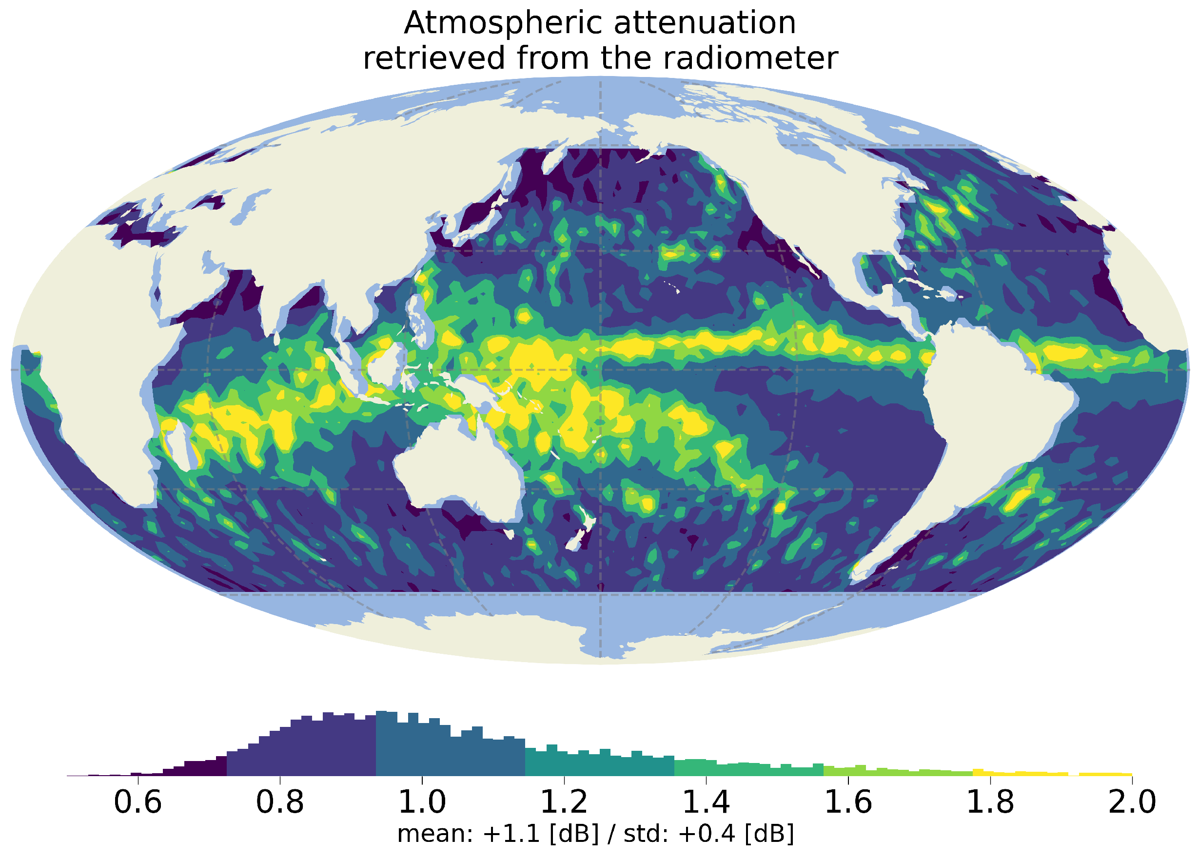
2.1. Ka Band Atmospheric Attenuation

The atmospheric attenuation (hereafter referred as $\Delta {\sigma }_0$) is the sum of a dry component $\Delta {\sigma }_0^{\mathrm{dry}}$ depending on pressure (p) and temperature (t), a wet component $\Delta {\sigma }_0^{\mathrm{wet}}$ proportional to the total column water vapour content (TCWV), a liquid component ($\Delta {\sigma }_0^{\mathrm{liq}}$) depending on the liquid water path (LWP) and a component $\Delta {\sigma }_0^{\mathrm{rain}}$ proportional to the rain rate (RR).

Lillibridge et al. (2014) [12] proposed a polynomial empirical relation of some atmospheric components to compute Ka band and Ku band attenuations from ECMWF analyses. However, this approach is limited for the study of short temporal and/or spatial-scale attenuation events since (1) it requires an interpolation between two successive analyses separated by 6 h, (2) the location of clouds and their associated liquid water content is not accurate as for any Numerical Weather Prediction (NWP) model and (3) the rain rate is not part of the analysis dataset when it is critical for the Ka band.

The microwave radiometer (MWR) on board the SARAL/AltiKa mission has a better spatial resolution (about 12 km) and provides retrievals of atmosphere-related parameters simultaneously to the altimeter observations. The wet tropospheric correction retrieved from the brightness temperatures (TB) shows very good performance as demonstrated in [28]. Nevertheless, due to the coarser spatial resolution and sampling compared with the altimeter, the radiometer $\Delta {\sigma }_0$ underestimates the amplitude of the attenuation over rain cells. As illustrated by Figure 1, the geographical distribution of the atmospheric attenuation retrieved by the radiometer is mainly driven by the distribution of the water vapor with values less than 2 dB. Figure 2 also shows how strong attenuation of the ${\sigma }_0$ (blue dots) are largely underestimated by the radiometer (brown solid line).

The originality of the current approach is to take benefit from a direct measurement of the variation of the Ka band altimeter backscattering coefficient, with a fine spatial resolution (about 4 km, slightly better than the PR on-board TRMM) combined to a very fine temporal sampling (40 Hz). As illustrated by Figure 2, the along-track ${\sigma }_0$ timeseries contain a fine spatial description of attenuation cells with a corresponding spatial sampling of about 175 m. The SARAL/AltiKa mission thus offers a unique opportunity to study the small-scale variation of the Ka band $\Delta {\sigma }_0$.

Tournadre (2006) already estimated the characteristics of rain cells from Jason-1 and Envisat Ku band rain attenuation ${\Delta {\sigma }_0}_{\mathrm{Ku}}$, essentially obtained from the difference between the 1 Hz Ku band and C or S band ${\sigma }_0$: any measurements where ${\Delta {\sigma }_0}_{\mathrm{Ku}}$ is larger than 0.5 dB when LWP is larger than 0.2 ${\mathrm{kg}·\mathrm{m}}^{-2}$ are considered under rainy conditions. The rain cell chord distribution (RCCD) is established from the number of consecutive measurements under rainy situations. Indeed, altimeters do not directly measure the diameter of the rain cell but its chord, since the altimeter track randomly samples the two-dimensional rain cells. Sauvageot et al. (1999) [19] established a relation between the RCCD and the rain cell diameter distribution (RCDD). The mean chord of the RCCD and the mean diameter of the RCDD are proportional, with a factor of $\frac{2}{\pi }$, assuming circular-shaped rain cells. This relation is useful to translate one-dimensional information as provided by SARAL/AltiKa to two-dimensional cases that will be encountered by the future SWOT mission, even if the actual shape of rain cells is more likely to be elliptical over ocean [22] or even without any particular shape [16]. The statistics of rain rates and cells sizes provided by [23] are mostly confirmed by the existing literature, but with some limitations compared with the current proposed approach, being (1) the spatial resolution of the Topex and Jason-1 altimeters were coarser than for AltiKa, (2) the study was based on 1 Hz measurements (separated by 6 km) and (3) the Ku band is seven times less sensitive to rain than the Ka band. The following section describes the new algorithm used to characterize attenuation cells directly from the Ka band SARAL/AltiKa altimeter from the 40 Hz Ka band ${\sigma }_0$ timeseries.

2.2. Description of the Datasets

This study makes use of the dataset provided by the Prototype for Expertise on AltiKa for Coastal, Hydrology and Ice (PEACHI) initiated to deliver a long series of research-grade Level 2 product notably featuring an innovative retracking algorithm [29]. All the parameters defined below are included in this dataset, which is available at the high data rate of 40 Hz and at the compressed data rate of 1 Hz.

The period of interest covers the whole year 2015, from AltiKa cycle 20 (starting on the 8 of January 2015) to cycle 30 (ending on the 28 January 2016). It corresponds to the strong 2014–2016 El Ni$\tilde{\mathrm{n}}$o event. At global scale, the precipitation over ocean is larger than the long-term average, in keeping with the five previous years. The increase in rainfall was particularly high in the Pacific Ocean over the Inter-Tropical Convergence Zone (ITCZ), western and eastern Pacific Ocean and over the Indian Ocean. On the contrary, a strong negative rainfall anomaly was observed over the seas of the Maritime Continent and a below-normal precipitation occurred in the northern and southern Pacific Oceans [30]. The question of the representativity of this particular year with respect to an average situation is difficult to answer considering the high inter-annual and spatial variability of the precipitation. Still, the results presented here should provide useful information for the future missions.

A specificity of our approach is to base our analysis on the ${\sigma }_0$ timeseries estimated from the adaptive retracking applied on 40 Hz waveforms. This new solution is reliant on the Nelder–Mead method implemented with an exact likelihood criterion for low resolution mode measurements [31]. The main benefit for the current study is the capability of this retracking to provide a ${\sigma }_0$ less correlated to the other parameters retrieved from the waveform (range and significant wave height): the backscattering coefficient statistics are more representative of atmosphere and surface conditions.

2.3. Definition of the ACECAL Algorithm

Figure 2 shows a typical rain cell selected according to the criteria detailed in the following paragraph. On the abscissa is reported the distance from the first measurement. The blue dots show the 40 Hz ${\sigma }_0$ timeseries retrieved from the adaptive retracking. The segments are selected based on the MP rain flag that is raised along about 40 km (see the orange dotted line). The variation of the ${\sigma }_0$ can generally be explained either by surface or by atmospheric conditions. Since both share a common range of spatial scales and amplitude of their impact on the backscattered signal, it is difficult to discriminate between the two, for instance to distinguish between the scattering due to large surface wave height and the attenuation due to rain. Large-scale variation of the atmospheric attenuation is usually well captured by the retrieval from the radiometer observations. However, the combination between an empirical approach for the estimation and the coarse spatial resolution of MWR observations (see the 37 GHz TB values in solid violet lines) leads to a clear underestimation of the atmospheric attenuation under rainy conditions (brown solid line). Those conditions represent less than 10% of the global atmospheric conditions and the neural network used for the operational processing  as any other empirical approaches, underperforms for events so underpopulated in the learning database (see Obligis et al. (2009) [32] for the response of the neural network to underpopulated events).

Indeed, on top of the large-scale variation, the internal structure of the rain cell is seen through the Gaussian-shaped peaks with an attenuation of about 5 dB, with respect to the background. The 37 GHz TB value of more than 220 K clearly identifies this pattern as the result of atmospheric conditions, but the retrieved atmospheric attenuation is only of about 4 dB, only 2 dB above the estimated background. These situations are typical of a one-dimensional cut of a two-dimensional precipitation field. As highlighted by [33] when he defines a rain cell model to assess its impact on altimeter waveform, a Gaussian shape for the rain-rate falloff, even if idealized, is well adapted for rain rates up to 50 mm·h⁻¹ [18].

Setting out from this premise, the core of the Attenuation CElls Characterization ALgorithm (ACECAL) relies on a non-linear least-square fit of the ${\sigma }_0$ timeseries, where the fitting model uses a combination of a 3-degree polynomial and a pre-defined number of Gaussians. The implementation of this approach is performed using the LMFIT python library [34]. This algorithm provides an estimate of the location, the chord and the amplitude of the rain cells that impact the Ka band ${\sigma }_0$. The following paragraphs describe the pre-processing applied before the selection of segments where rain conditions occur, the processing that leads to the characterization of the attenuation cells and its limitations.

2.3.1. Pre-Processing

Several editing criteria are applied to the measurements to select segments identified as under rain events conditions, before running ACECAL. The parameters in italic refer to the name of the fields in the PEACHI products available in NetCDF format. The selection criteria are summarized in

Table 1. Criteria for the selection of segments impacted by rain and the selection of attenuation cells within those segments.

Pre-Processing
Parameter	Criteria	Comment
surface_type	== 0	open ocean
ice_flag	== 0	no sea ice
distance_shoreline	≥50 km	no land contamination on TB
off_nadir_angle_pf	== 0	no platform maneuvers or depointing
Post-Processing
Parameter	Criteria	Comment
trailing_edge_variation_flag_40hz	== 1	MP flag raised (potential rain event)
sig0_adaptive_40hz - atmos_corr_sig0_40hz	<15 db	no bloom
short-scales/large-scales windows size	1.5 km/30 km	to select attenuation cells
minimum amplitude of the attenuation due to rain cells	≥0.5 dB	to ensure the robustness of the fit
value of 37 GHz TB at the maximum attenuation	≥175 K	to ensure the detection of rain event

.

In order to select open ocean conditions only, the following values or thresholds are used. The measurement should lie over ocean (surface_type == 0), not over identified sea ice (ice_flag == 0 and abs(latitude) <= 60°) and at a distance larger than 50 km from the coast (distance_shoreline > 50 km). This latter criterion ensures that the brightness temperatures observed by the MWR are not impacted by the coast, which leads to an increase in the value that could be falsely interpreted as an increase in the precipitations. The value of ${\sigma }_0$ and the robustness of the rain flag are also impacted by orbit maneuvers, leading to mispointing periods: the off-nadir angle of the platform should be null (off_nadir_angle_pf == 0).

The MP rain flag is used to select the segments where rain conditions occur. In order to avoid potential sharp cuts of the gaussians at the borders of selected zone, a margin of 10 km or 15% of the segment size is added on both sides, respectively, for a size of less or more than 100 km.

Finally, the ${\sigma }_0$ timeseries should obviously not be corrected from the atmospheric attenuation. Since it is the case in PEACHI products, the atmospheric attenuation (atmos_corr_sig0_40hz) is systematically subtracted to the corrected ${\sigma }_0$ (sig0_adaptive_40hz) before the analysis.

2.3.2. Processing

As pointed out by Tournadre et al., 2015 [15], the MP flag is also sensitive to bloom events, where the ocean surface is smooth, resulting in large ${\sigma }_0$ values and short-scale variation of the off-nadir angle. The authors rely on the radiometer LWP to discriminate between actual rain events and surface blooms: any measurements flagged by the MP approach with LWP below 0.1 kg·m⁻² are classified as bloom events. As it happens, high values of ${\sigma }_0$, representative of bloom conditions, are associated with high values of 37 GHz TB, these latter being directly related to the radiometer LWP. It is thus chosen here to apply a maximum threshold of 15 dB directly to ${\sigma }_0$: if it exceeds this limit within the selected segment, the segment is discarded. The value of the threshold is arbitrary but has a weak impact on the eventual robustness of the results thanks to the sequencing of filtering steps presented below.

If the segment is selected, the first step consists on determining the number of peaks and the index of their maximum. The peaks are isolated from a residue obtained by the difference between a short-scales and a large-scales median filter applied to the original ${\sigma }_0$ timeseries. The small-scale filter has a window size of about 1.5 km (10 successive measurements), removing the small-scale noise and allowing a better location of the peak maxima. The large-scale filter has a window size of 30 km, removing the large-scale variations of the signal. The size of these windows has been chosen in agreement with the global distribution of the rain cell size as established in the literature. Goldhirsh (1983) [35] shows that less than 10% of the cells corresponding to light rain rate events (2 mm·${\mathrm{h}}^{-1}$) have a size larger than 30 km, less than 4% for rain rates of 5 mm·${\mathrm{h}}^{-1}$. For Begum et al. (2009) [20], it is even less than 1% for the same rain rate. For larger rain rates, the maximum size is below 15 km. The sub-segments containing peaks are isolated from the sections where the residue is larger than 0.5 dB. If this criterion is not fulfilled, the segments are discarded. This limit of 0.5 dB has been selected to reinforce the distinction between surface and atmospheric impact on the ${\sigma }_0$. As pointed out in the following section, this limit could be relaxed in a future version of the ACECAL approach. Over each selected section, the position of the maximum is found.

To select rainy conditions amongst the different conditions where the MP flag is raised, we choose here to apply a threshold on the 37 GHz TB rather than on the LWP. The retrieval algorithm for the LWP is depending on the ${\sigma }_0$ and as said above, with values potentially out of the optimal range of validity of the neural network under rainy conditions. A threshold on the 37 GHz TB, being more sensitive to LWP than the 23.8 GHz channel, is more straightforward and independent from any retrieval algorithm, including the retracking algorithm used to estimate the ${\sigma }_0$. Only the sections where the maximum of the cell corresponds to a value of the 37 GHz TB larger than 175 K are eventually selected (tb_ka > 175 K). This value has been established empirically based on the monitoring of both the 37 GHz TB and the surface wave height, and offers the best robustness, even if some actual cells may be not selected.

The non-linear model is defined as the combination of a 3-degrees polynomial and a number of Gaussians equal to the number of selected peaks. The initial positions of the Gaussians are used as initial values. The final quality of the fit being weakly dependent on the initial values of the amplitude and the sigma of the Gaussian, their values are fixed, respectively, to −250 and 2, as recommended by the LMFit library. The fit is then applied to the non-filtered ${\sigma }_0$ timeseries inside the whole segment.

Figure 2 shows the result of the fit as the red solid lines, the dashed black lines referring to the polynomial components. On these examples, the fit succeeds to reproduce the variation of the background and the shape of the peaks. The figure also illustrates how the ACECAL approach provides a finer description of the situation within the rainy area than the MP flag: the actual number of observations within the attenuation cell may be larger than the observations flagged by the MP approach and the inner structure is clearly not uniform. The location of the maximum and the width of the peaks are well estimated, with small uncertainties (less than 0.5 dB and less than 2 km, respectively).

The location of the minimum and the value of the minimum are computed for each Gaussian detected within a segment. The full width at half maximum (FWHM $\approx 2.35482\sigma$) and the six-$\sigma$ full width (FW6S = 6$\sigma$) are deduced from the standard deviation of the Gaussian $\sigma$.

The size of the rain cell is defined by the distance covered by the sum of the FW6S of each individual peak, accounting for overlapping if it occurs. This size thus defined is close to the size where the MP flag is raised in the cases illustrated by the middle and the bottom panel of Figure 3. In the case illustrated by the top panel, the size of the cell is computed as the sum of the width each individual peak. Under this particular condition, those peaks should have been considered individually since they are clearly individual cells. This is a current limitation of ACECAL that does not include a criterion on the separability of the peaks.

In the case of the retrieval of a two-dimensional SSH as with the SWOT mission, the distribution of rain cells will appear as areas with stronger attenuation over a background at a given amplitude. In the perspective of future validation activities that will have to discriminate between surface and atmospheric signals, it is valuable to characterize the difference between the background and those areas. The maximum of the attenuation within a peak is thus defined as the difference between the minimum value of ${\sigma }_0$ and the polynomial fit at the same location. It better characterizes the contrast between the short-scale impact of the rain cells over the large-scale varying backscattering coefficient than if it would have been defined as the absolute value of the ${\sigma }_0$ at the maximum.

During the year 2020, 56,000 rain cells were detected by the ACECAL method, and within these rain cells, 84,500 peaks were identified.

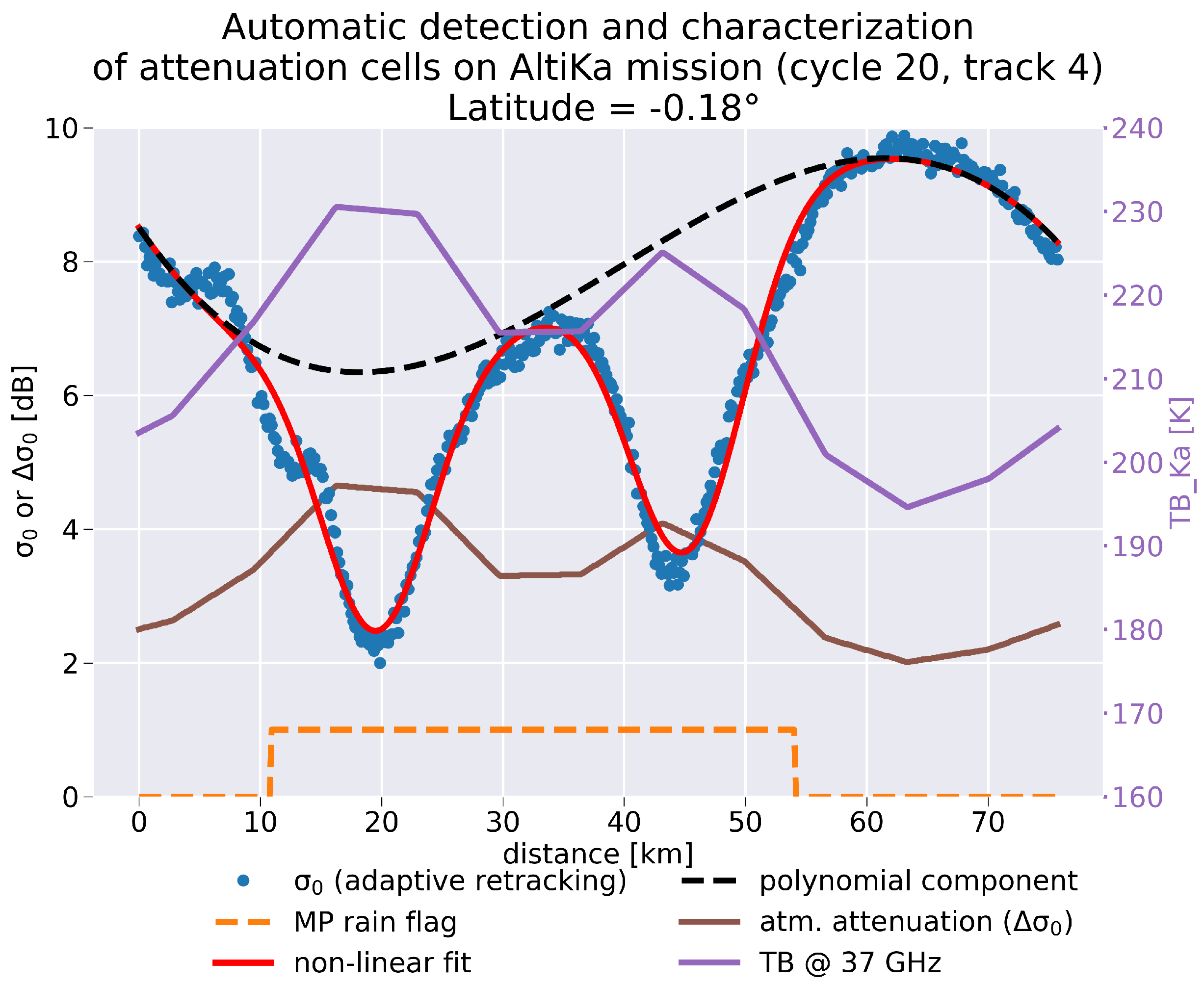
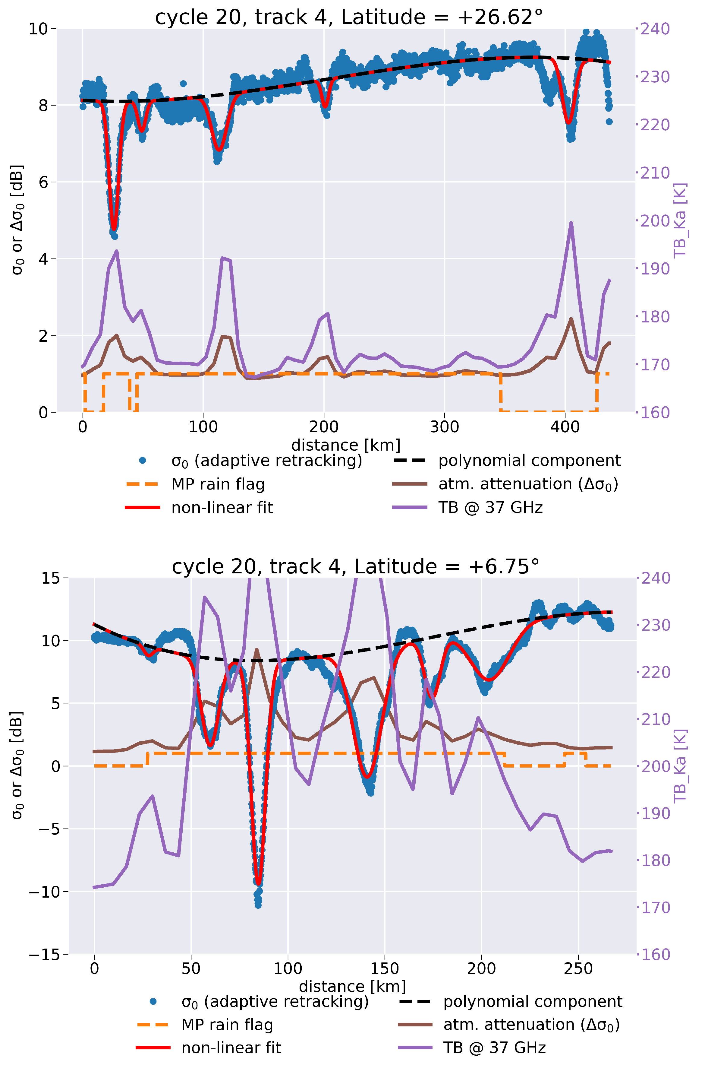
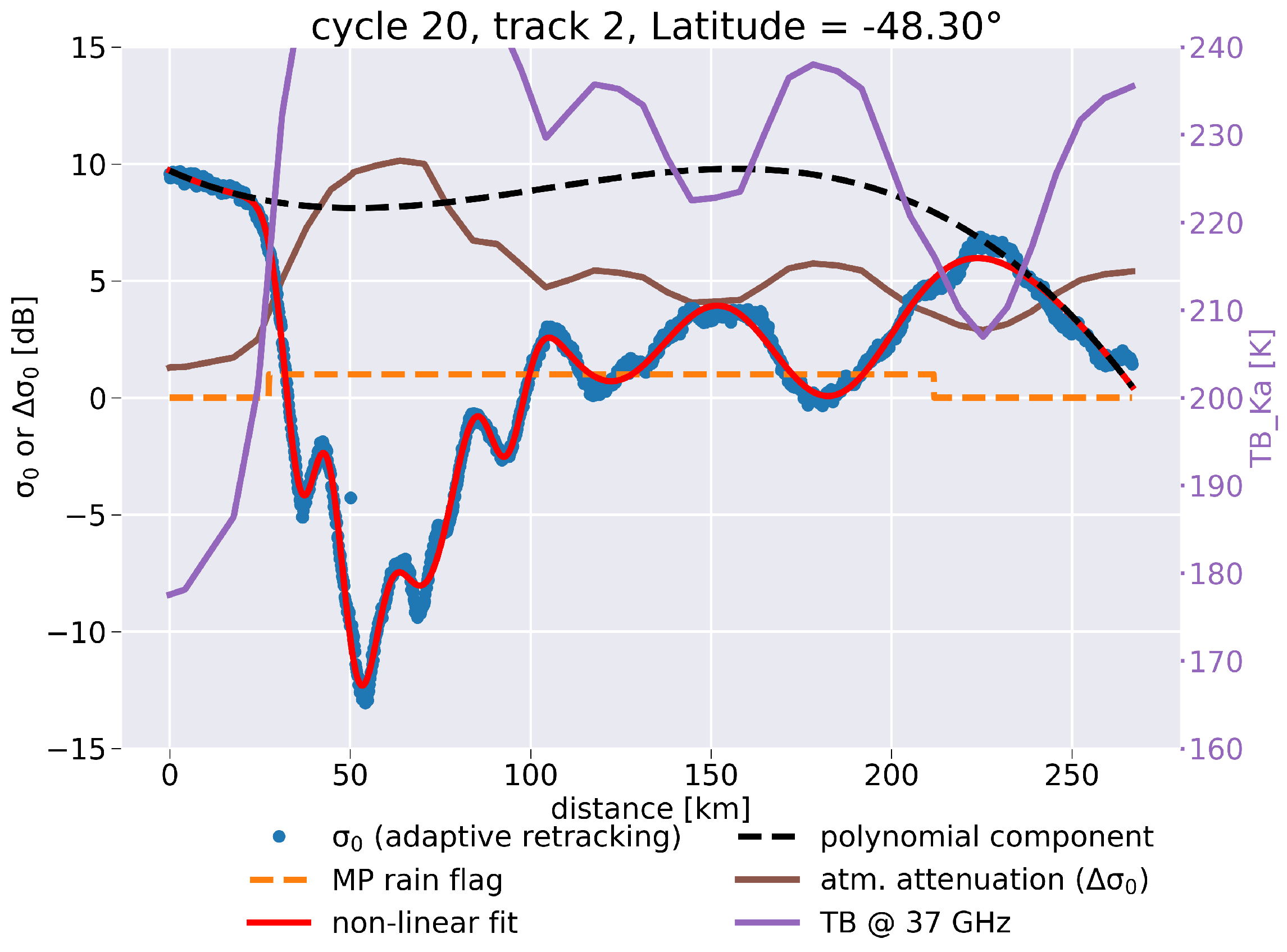
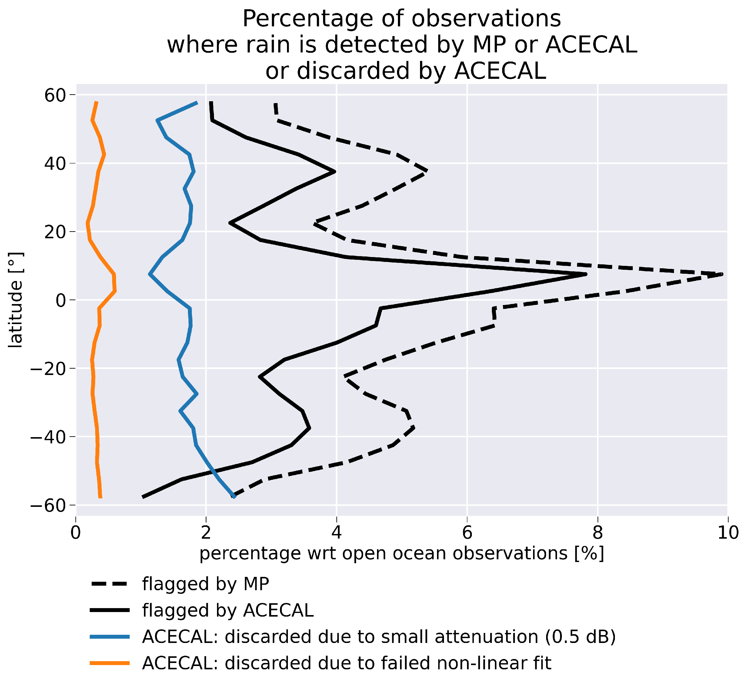
2.3.3. Illustrative Cases and Zonal Distribution of Occurrences

Figure 3 illustrates how the method succeeds to fit complex conditions and provides a finer level of information than given by the MP flag. The top panel shows a long segment of 400 km, where the MP flag is raised but the ACECAL approach detects only a limited distant cell, the last one lying in an area where the MP flag is actually not raised. Even when the situation is complicated by the presence of large rain rates (associated with 37 GHz TB values larger than 230 K), the ACECAL approach provides a fit very close to the ${\sigma }_0$ timeseries (see the middle and bottom panels). Nevertheless, the polynomial fit may sometimes not reflect the actual variation of the background, and the resulting attenuation may be overestimated, as shown by the bottom panel.

The percentage of 40 Hz observations flagged, respectively, by the MP approach and the ACECAL method with respect to the total number of 40 Hz observations over open ocean (defined by the criteria of the pre-processing, see Table 1) are of the same order, as illustrated by Figure 4. The zonal variation for the MP flag is close to the results presented in Figure 5 in Tournadre et al., 2015 [15]: a maximum of 10%s over the ITCZ, with two secondary maxima at 5% around 40°N and 40°S along the mid-latitude storm tracks. Only the asymmetry between Northern and Southern hemisphere in terms of climatological distribution of the precipitation is not seen here, but may be due to some particularity of the year 2015.

The percentage of observations detected by ACECAL is smaller by about 1%. As said above, the percentage of observations where the non-linear fit failed to converge is small, no larger than 0.6%, even at its maximum in the ITCZ region. The percentage of observations initially flagged by the MP approach but not selected in input to ACECAL is close to 2% with a small zonal distribution as well. This smaller percentage is explained by the fact that the ACECAL processing is relying on the MP flag but apply a stringent criterion on the minimum attenuation for a cell to be detected. However, there may be some compensation effects between peaks detected outside the area (larger number of flagged observations) and narrow peaks within the area (smaller number of flagged observations). The distinction between these two situations is not investigated further within the frame of the current study. Amongst the leads for further improvement of the ACECAL approach, it could be interesting to propose a solution that is not dependent on the MP flag and to assess if the lower threshold of 0.5 dB on the attenuation could be overcome.

3. Amplitude and Size of Attenuation Cells Retrieved from SARAL/AltiKa Mission

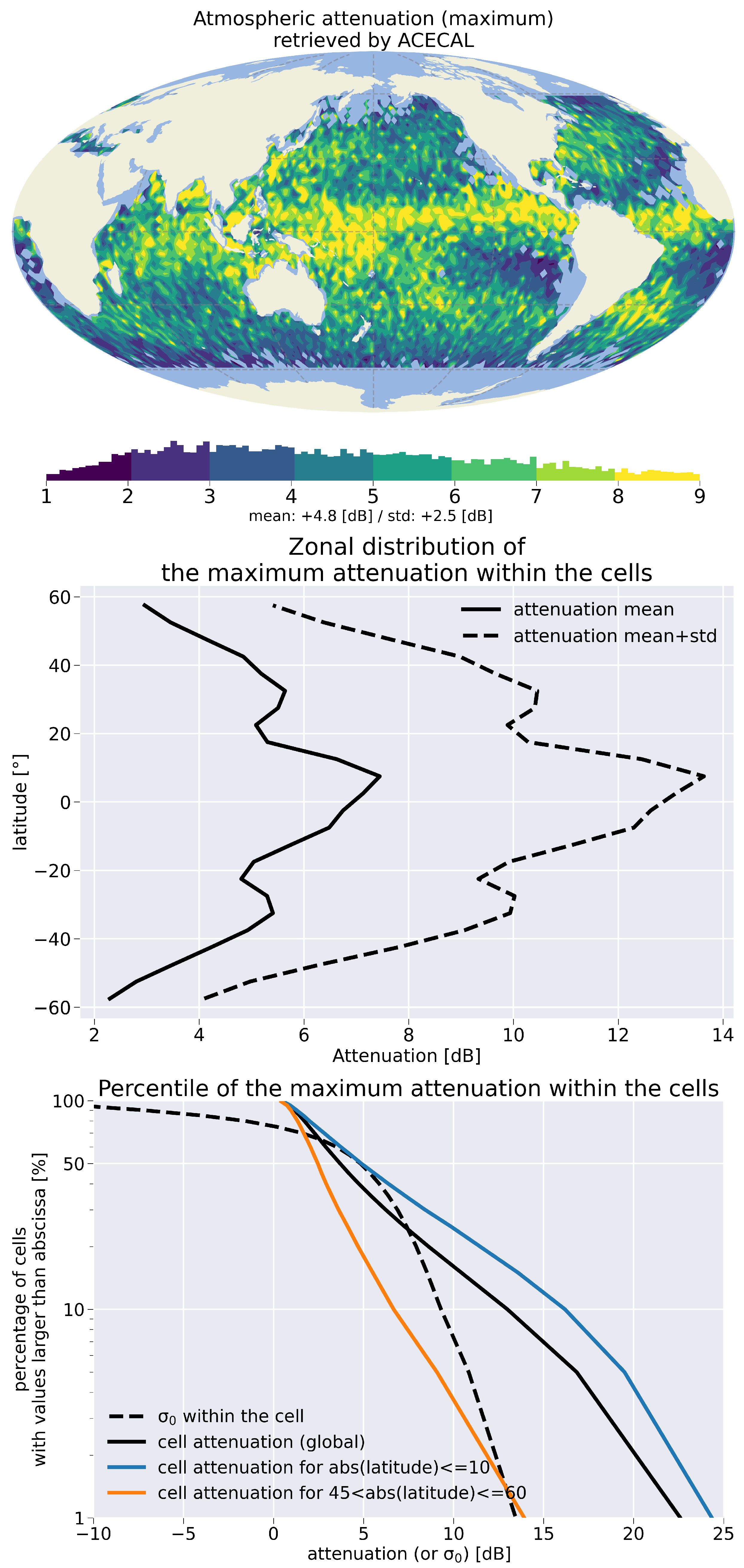
3.1. Amplitude of Attenuation Cells

Table 2. Characteristic of rain cells retrieved by the ACECAL approach (global statistics).

Attenuation at Peak Maximum (Rain Rate [mm·h−1] @ 6 km Thickness; 3 km Thickness)
99th percentile	90th percentile	median	10th percentile	1st percentile
0.5 dB (<1; <1)	1.0 dB (<1; <1)	3.5 dB (1.5; 2.4)	13 dB (6; 9)	23 dB (10; 16)
Rain Cell Diameter
99th percentile	90th percentile	median	10th percentile	1st percentile
5 km	8.5 km	15 km	41 km	103 km
Peak Diameter (FWHM)
99th percentile	90th percentile	median	10th percentile	1st percentile
1.5 km	3 km	5 km	10 km	20 km

summarizes the results discussed hereafter. Figure 5 shows different metrics that characterize the relative attenuation (with respect to the fitted background) at the maximum of the peaks detected with ACECAL, thus corresponding to a worst-case scenario.

The geographical distribution of the attenuation is consistent with the strongly zonal distribution of water vapour and precipitation (Figure 5, top panel). The amplitude is four times larger than the attenuation computed from the radiometer (see Figure 1) or using NWP analyses (Figure 2 in Lillibridge 2014); based on the 40 Hz observations provided by the altimeter instead of the coarser and sparser radiometer retrievals of the attenuation (or even coarser estimations from the model), it better reflects the actual impact of the rain onto the backscattering coefficient and consequently illustrates the benefits of the ACECAL approach. As expected, over dry regions where upwelling occurs, no cells are detected or with attenuation of the order of 1 dB. On the opposite, the maximum attenuation is larger than 8 dB along the ITCZ but also over the regions impacted by the Indian monsoon. Other regions of particular interest for the altimetry are also impacted. For instance, over the Brazil current, over the South Atlantic Convergence Zone, the attenuation shows values larger than 8 dB.

The zonal distribution of the amplitude (Figure 5, middle panel) shows that the averaged amplitude varies from 2 dB at high latitudes to about 7 dB at ITCZ, but considering the average plus the standard deviation, the amplitude is about 6 dB for latitudes below 40° and can reach 14 dB in the ITCZ.

The bottom panel of Figure 5 displays the percentiles of the absolute value of ${\sigma }_0$ at the maximum of the peaks (see the dotted black lines): for 10% of the strongest attenuation peaks, the $sigm{a}_0$ can reach values lower than −7 dB, to be compared with a value of +10 dB under clear-sky conditions. Now focusing on the relative attenuation (see the solid black line), the median at the maximum of the attenuation peaks is about 3.5 dB and 10% of the peaks have a maximum attenuation of 13 dB. As illustrated by the middle panel, the attenuation strongly depends on the latitudes and the orange and blue solid lines show the attenuation at high latitude (above 45°) and below 10°, respectively: the 10th percentile is larger than 15 dB over the equatorial region.

The statistics on the attenuation can be roughly translated to hourly rain rates in order to validate the results. The Marshall–Palmer parameterization of [36] is used for a frequency of 35.75 GHz. Assuming a thickness of 6 km for the rain layer, the median attenuation for the peaks of 3.5 dB corresponds to a rain rate of about 1.2 mm·h⁻¹ and the 1st percentile of 23 dB to a rain rate of about 8 mm·h⁻¹. Table 2 also contains the results assuming a 3 km thickness: [16] uses PR measurements with a similar spatial resolution and exhibits a double peak of the thickness distribution over the ocean at 3 km for shallow isolated precipitation and 6 km for deep rain cells. Those results for SARAL/AltiKa are in agreement with [16], who reported an average rain rate over ocean varying between 0.4 mm·h⁻¹ and 8 mm·h⁻¹ with a peak at 1 mm·h⁻¹, even if the two datasets cannot be directly compared. Ref. [16] provides results limited to the Tropics and averaging all rain conditions when the results presented in Table 2 are extended up to high latitudes but concerns the maximum attenuation within the peaks. The statistics are also in good agreement with the results established from the Ku band altimetry missions by [23] where the rain rate varies between 1.5 mm·h⁻¹ and 10 mm·h⁻¹, with a peak around 2 mm·h⁻¹.

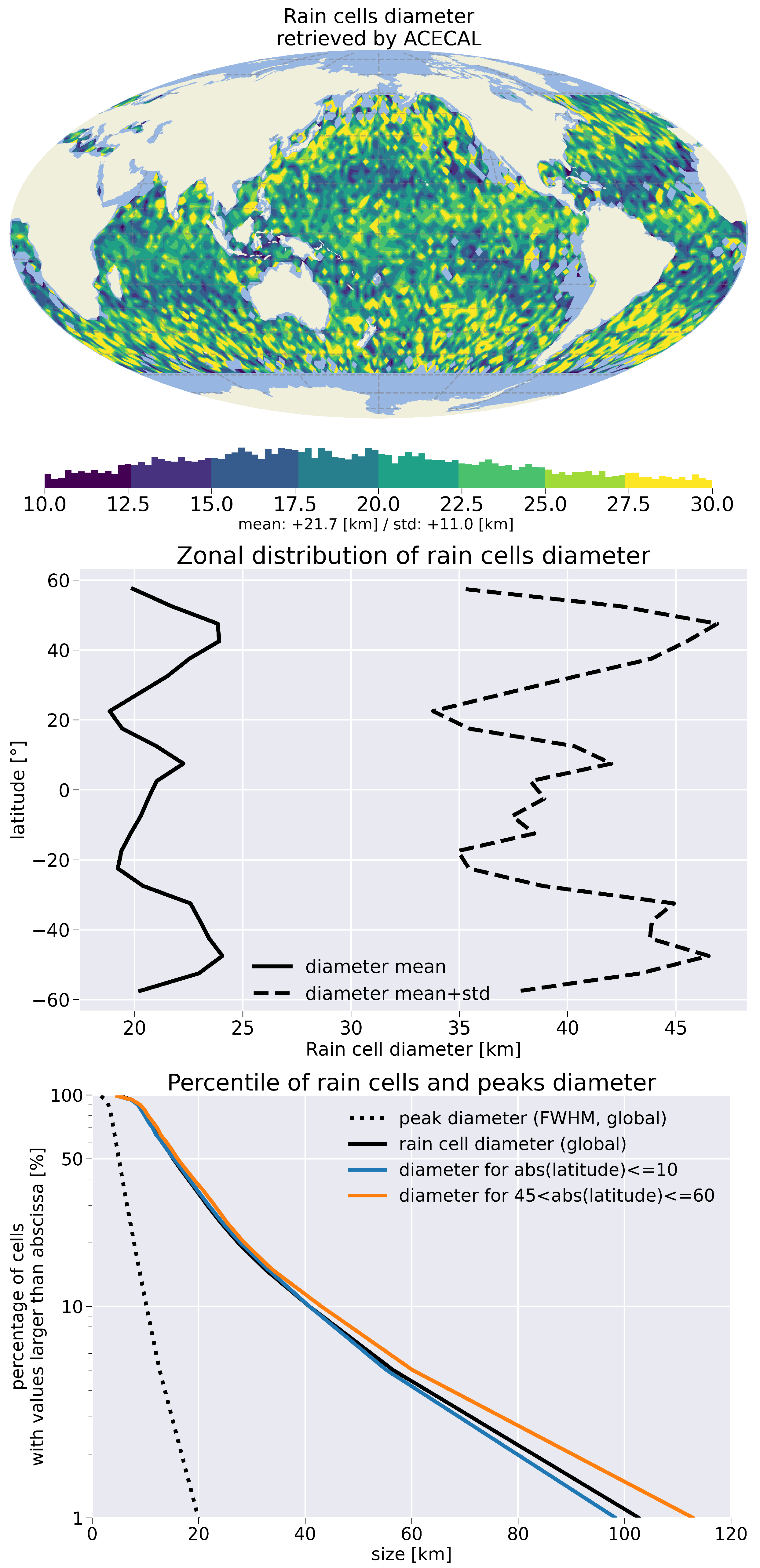
3.2. Diameter of Rain Cells

The estimation of the rain cell chord length provided by ACECAL is translated to the equivalent circular-shaped diameter using the relation established by [19]. The top panel of Figure 6 displays the geographical distribution of this diameter. The larger cells are detected at high latitudes associated with smaller attenuation. As shown by the zonal distribution of the size (Figure 6, middle) and as highlighted by Nesbitt et al. (2006) [21], a minimum is observed around ±20° latitude, above the semipermanent highs associated with clear sky conditions. Nevertheless, the contrast between tropical regions and high latitudes is small on average: the mean diameter is about 20 km in the Tropics against less than 25 km for latitudes around 40°, along the storm track. Considering now the average plus the standard deviation, the contrast is slightly larger, with larger variability at higher latitudes and a diameter larger than 45 km. The bottom panel of Figure 6 displays the percentile of the rain cells diameter (solid lines). On the contrary to the previous metrics, the distribution of the diameter shown here is not impacted by any averaging. The median of the diameters is equal to 15 km and rain cells with diameters larger than 40 km represent about 10% of the population. The difference between the percentiles of the diameters for rain cells lying around the Tropics (solid blue line) or at higher latitudes (orange solid line) is small.

Those results are also in agreement with previous studies. Fu et al. (2020) [16] computes a median length and width of 20 km and 15 km over ocean over the region covered by TRMM, respectively, close to the median found in the present study. Nesbitt et al. (2006) [21] discussed more in details the geographical distribution of the size of rain cells (see their Figure 8). The feature’s maximum dimension (FMD) is computed as twice the major axis of the ellipse that fits the rain cell: the maximum of the FMD is located over the ITCZ and in the subtropics. Over ocean, it varies between 10 km and 20 km, with a minimum of about 7 km over the dry upwelling regions. Those results are slightly more contrasted than the distribution shows in Figure 6 but both the FMD and the mean rain area shows maximum along the ITCZ and at higher latitudes around 35°. Indeed, it is confirmed by the study of [37] who computed the distribution of precipitation system size using the Integrated Multi-SatellitE Retrievals for the Global precipitation measurement (IMERG) level 3 gridded product. Figure 1 shows that the median precipitation system size is large at latitude above 40°N and 40°S. Tournadre (2006) [23] also displays the geographical distribution of the slope of the RCCD. The corresponding mean diameter of the rain cells is consistent with the previous results over the Tropics with a value of about 16 km but this value drops to 4 km to 6 km at higher latitudes. Since the rain rate is lower at higher latitude, this difference may be due to a weakness of the approach based on Ku band measurements, which are less sensitive to precipitations.

The ACECAL approach also provides information on the diameter of the internal peaks. We chose to display in Figure 7 the metrics for the FWHM of the peaks, which is more consistent with the maximum attenuation shown in Figure 5. At a global scale (top panel of Figure 7), the geographical distribution is smooth: the diameters of the peaks are larger than 6 km at latitudes larger than 40°, with a minimum along the semipermanent highs, illustrated by the zonal average as well (bottom panel of Figure 7). As seen in the bottom panel of Figure 6 by the dotted lines, at a global scale, the median of the peak diameter is 5 km and 10% of the peaks have a diameter larger than 10 km.

4. Conclusions

The use of Ka bands for radar altimeter allows a reduction in the spatial resolution from about 15 km with the historical Ku band instruments to about 4 km. However, it also comes with a larger sensitivity to the atmospheric attenuation, especially under rainy conditions. As the radiometers on-board altimetry mission have a coarser spatial resolution (12 km for MWR on-board SARAL/AltiKa), a new approach is proposed here, based on the 40 Hz ${\sigma }_0$ (one point every 175 m), to characterize the impact of rain cells onto the measurements and anticipate the availability of the observations performed by future two-dimensional swath Ka band altimeters. The ACECAL approach combines low-filtering and non-linear fit to retrieve the amplitude of the atmospheric attenuation at the Ka band, the size and the occurrences of rain cells. The conclusion of this work can be discussed according to two different applications.

First, the robust characterization of rain cells can be used to draw some guidelines for the future altimetry missions based on the Ka band as SWOT (oceanography and terrestrial surface water), SKIM (oceanic currents) or SMASH (land water bodies) missions. At global scale and for a nadir instrument, the number of observations strongly impacted by the atmospheric attenuation is limited, with a proportion of observations belonging to rain cells lying between 5% and 10%: this result first shown by Tournadre et al., 2015, is confirmed here with a different method. However, concerning the atmospheric attenuation within the rain cells, the previous studies relied on radiometer observations or model analyses and thus underestimated the actual amplitude of the atmospheric attenuation caused by rain by a factor four: the global median attenuation under-rainy situation is about 3.5 dB and 10% of the attenuations are larger than 13 dB, as illustrated by Figure 5. One originality of the method presented here is also to provide robust statistics on the rain cells diameter, their occurrences and geographical distribution. The median is 15 km, 10% of the rain cells have a size larger than 41 km, and the size is also larger at higher latitudes than over the tropics.

Now, for the future swath missions, both the occurrences and the maximum of atmospheric attenuation could even be larger as the probability to cross a strong precipitation event (as tropical storm) increases. Generic conclusions can yet be drawn using the geographical distribution of the size and the amplitude: that some regions of particular interest for oceanography as Gulf Stream, North Pacific or Brazil currents could be systematically affected in terms of data availability or degraded budget errors. The results presented here could help to better define the functioning point of the future Ka band radar altimeters with a larger reliability in order to maintain the overall availability of the altimetric observations. For instance, the distribution of size and amplitude established here could be used by the prototypes developed to assess the performances of future missions: added to the simulations of the geophysical context, it could improve the accuracy of the budget errors by including degraded cases caused by the atmosphere and help to the definition of future validation metrics to detect those atmospheric events. Another application of the ACECAL approach to the improvement of the current and future altimetry system, is the perspective of a better retrieval of the atmospheric attenuation, currently poorly estimated from the radiometer observations. The pattern index of atmospheric attenuation from the 40 Hz flagged measurements could be used as a basis for an empirical approach that would estimate the attenuation directly from the altimeter backscattering coefficient timeseries.

Secondly, this work demonstrates the capability of the Ka band radar altimeter to provide observations strongly consistent with the measurements provided by missions dedicated to the precipitations, as the precipitation radar on-board the TRMM mission. The retrieval of rain rate and rain cell size but also the characterization of the internal peaks, if they are distributed as secondary products of altimetry missions would certainly benefit the community, especially if the approach can be generalized to the future two-dimensional swath altimetry missions.

Yet, some aspects of the ACECAL approach could be improved in order to increase its robustness. A first lead would be to assess if there is some interest to apply it independently from existing rain flags: whether ACECAL would provide more robust detections of rain events, minimizing the number of missing events is still to be investigated. A major step would be also to estimate the rain rate from the attenuation provided by this method: the accuracy of the computation of the relative attenuation with respect to the fitted background has to be assessed and the most suitable retrieval method has to be selected. Here again, the validation would benefit from the PEACHI dataset, which also contains rain rates match-up from SSMI-S and WindSat missions.

References

1. Escudier, P.; Couhert, A.; Mercier, F.; Picard, B. Satellite radar altimetry: Principle, accuracy and precision. In Satellite Altimetry over Oceans and Land Surfaces; Stammer, D., Cazenave, A., Eds.; Taylor & Francis Inc.: Boca Raton, FL, USA, 2018; Chapter 1; pp. 1–70. [Google Scholar]
2. Fu, L.L.; Christensen, E.; Yamarone, C.; Lefebvre, M.; Menard, Y.; Dorrer, M.; Escudier, P. TOPEX/Poseidon mission overview. J. Geophys. Res. Atmos. 1995, 99. [Google Scholar] [CrossRef]
3. Heslop, E.E.; Sánchez-Román, A.; Pascual, A.; Rodríguez, D.; Reeve, K.A.; Faugère, Y.; Raynal, M. Sentinel-3A Views Ocean Variability More Accurately at Finer Resolution. Geophys. Res. Lett. 2017, 44, 12367–12374. [Google Scholar] [CrossRef] [Green Version]
4. Quartly, G.D.; Guymer, T.H.; Srokosz, M.A. The Effects of Rain on Topex Radar Altimeter Data. J. Atmos. Ocean. Technol. 1996, 13, 1209–1229. [Google Scholar] [CrossRef] [Green Version]
5. Tournadre, J.; Morland, J.C. Effects of rain on TOPEX/Poseidon altimeter data. IEEE Trans. Geosci. Remote Sens. 1997, 35, 1117–1135. [Google Scholar] [CrossRef]
6. Quartly, G.D. Sea state and rain: A second take on dual-frequency altimetry. Mar. Geod. 2004, 27, 133–152. [Google Scholar] [CrossRef] [Green Version]
7. Tournadre, J. Validation of Jason and Envisat altimeter dual frequency rain flags. Mar. Geod. 2004, 27, 153–169. [Google Scholar] [CrossRef]
8. Tran, N.; Obligis, E.; Ferreira, F. Comparison of two Jason-1 altimeter precipitation detection algorithms with rain estimates from the TRMM Microwave Imager. J. Atmos. Ocean. Technol. 2005, 22, 782–794. [Google Scholar] [CrossRef]
9. Steunou, N.; Desjonquères, J.D.; Picot, N.; Sengenes, P.; Noubel, J.; Poisson, J.C. AltiKa Altimeter: Instrument Description and In Flight Performance. Mar. Geod. 2015, 38, 22–42. [Google Scholar] [CrossRef]
10. Verron, J.; Bonnefond, P.; Aouf, L.; Birol, F.; Bhowmick, S.A.; Calmant, S.; Conchy, T.; Crétaux, J.F.; Dibarboure, G.; Dubey, A.K.; et al. The benefits of the Ka-band as evidenced from the SARAL/AltiKa altimetric mission: Scientific applications. Remote Sens. 2018, 10, 163. [Google Scholar] [CrossRef] [Green Version]
11. Verron, J.; Bonnefond, P.; Andersen, O.; Ardhuin, F.; Bergé-Nguyen, M.; Bhowmick, S.; Blumstein, D.; Boy, F.; Brodeau, L.; Crétaux, J.F.; et al. The SARAL/AltiKa mission: A step forward to the future of altimetry. Adv. Space Res. 2021, 68, 808–828. [Google Scholar] [CrossRef]
12. Lillibridge, J.; Scharroo, R.; Abdalla, S.; Vandemark, D. One-and two-dimensional wind speed models for ka-band altimetry. J. Atmos. Ocean. Technol. 2014, 31, 630–638. [Google Scholar] [CrossRef]
13. Tournadre, J.; Lambin-artru, J.; Steunou, N. Cloud and Rain Effects on AltiKa/SARAL Ka-Band Radar Altimeter—Part I: Modeling and Mean Annual Data Availability. Science 2009, 47, 1806–1817. [Google Scholar] [CrossRef] [Green Version]
14. Tournadre, J.; Lambin, J.; Steunou, N. Cloud and rain effects on ALTIKA / SARAL Ka band radar altimeter. Part II: Definition of a rain/cloud flag. IEEE Trans. Geosci. Remote Sens. 2009, 47, 1818–1826. [Google Scholar] [CrossRef] [Green Version]
15. Tournadre, J.; Poisson, J.; Steunou, N.; Picard, B. Validation of AltiKa Matching Pursuit Rain Flag. Mar. Geod. 2015, 38, 107–123. [Google Scholar] [CrossRef]
16. Fu, Y.; Chen, Y.; Zhang, X.; Wang, Y.; Li, R.; Liu, Q.; Zhong, L.; Zhang, Q.; Zhang, A. Fundamental Characteristics of Tropical Rain Cell Structures as Measured by TRMM PR. J. Meteorol. Res. 2020, 34, 1129–1150. [Google Scholar] [CrossRef]
17. Mesnard, F.; Sauvageot, H. Structural characteristics of rain fields. J. Geophys. Res. Atmos. 2003, 108. [Google Scholar] [CrossRef]
18. Capsoni, C.; Fedi, F.; Magistroni, C.; Paraboni, A.; Pawlina, A. Data and theory for a new model of the horizontal structure of rain cells for propagation applications. Radio Sci. 1987, 22, 395–404. [Google Scholar] [CrossRef]
19. Sauvageot, H.; Mesnard, F.; Tenório, R.S. The Relation between the Area-Average Rain Rate and the Rain Cell Size Distribution Parameters. J. Atmos. Sci. 1999, 56, 57–70. [Google Scholar] [CrossRef]
20. Begum, S.; Otung, I.E. Rain cell size distribution inferred from rain gauge and radar data in the UK. Radio Sci. 2009, 44. [Google Scholar] [CrossRef]
21. Nesbitt, S.W.; Cifelli, R.; Rutledge, S.A. Storm morphology and rainfall characteristics of TRMM precipitation features. Mon. Weather Rev. 2006, 134, 2702–2721. [Google Scholar] [CrossRef] [Green Version]
22. Liu, C.; Zipser, E. Regional variation of morphology of organized convection in the tropics and subtropics. J. Geophys. Res. Atmos. 2013, 118, 453–466. [Google Scholar] [CrossRef] [Green Version]
23. Tournadre, J. Improved level-3 oceanic rainfall retrieval from dual-frequency spaceborne radar altimeter systems. J. Atmos. Ocean. Technol. 2006, 23, 1131–1149. [Google Scholar] [CrossRef]
24. Ardhuin, F.; Brandt, P.; Gaultier, L.; Donlon, C.; Battaglia, A.; Boy, F.; Casal, T.; Chapron, B.; Collard, F.; Cravatte, S.E.; et al. SKIM, a candidate satellite mission exploring global ocean currents and waves. Front. Mar. Sci. 2019, 6, 209. [Google Scholar] [CrossRef] [Green Version]
25. Blumstein, D.; Biancamaria, S.; Guérin, A.; Maisongrande, P. A potential constellation of small altimetry satellites dedicated to continental surface waters (SMASH mission). In AGU Fall Meeting Abstracts; American Geophysical Union: Washington, DC, USA, 2019; Volume 2019, p. H43N-2257. [Google Scholar]
26. Durand, M.; Fu, L.L.; Lettenmaier, D.P.; Alsdorf, D.E.; Rodriguez, E.; Esteban-Fernandez, D. The surface water and ocean topography mission: Observing terrestrial surface water and oceanic submesoscale eddies. Proc. IEEE 2010, 98, 766–779. [Google Scholar] [CrossRef]
27. Biancamaria, S.; Lettenmaier, D.P.; Pavelsky, T.M. The SWOT Mission and Its Capabilities for Land Hydrology. Surv. Geophys. 2016, 37, 307–337. [Google Scholar] [CrossRef] [Green Version]
28. Picard, B.; Frery, M.L.; Obligis, E.; Eymard, L.; Steunou, N.; Picot, N. SARAL/AltiKa Wet Tropospheric Correction: In-Flight Calibration, Retrieval Strategies and Performances. Mar. Geod. 2015, 38, 277–296. [Google Scholar] [CrossRef] [Green Version]
29. Valladeau, G.; Thibaut, P.; Picard, B.; Poisson, J.C.; Tran, N.; Picot, N.; Guillot, A. Using SARAL/AltiKa to Improve Ka-band Altimeter Measurements for Coastal Zones, Hydrology and Ice: The PEACHI Prototype. Mar. Geod. 2015, 38, 124–142. [Google Scholar] [CrossRef]
30. Vose, R.; Becker, A.; Hilburn, K.; Huffman, G.; Kruk, M.; Yin, X. Precipitation [in “State of the Climate in 2015”]. Bull. Am. Meteorol. Soc. 2016, 97, S27–S28. [Google Scholar] [CrossRef] [Green Version]
31. Poisson, J.C.; Quartly, G.D.; Kurekin, A.A.; Thibaut, P.; Hoang, D.; Nencioli, F. Development of an ENVISAT altimetry processor providing sea level continuity between open ocean and arctic leads. IEEE Trans. Geosci. Remote Sens. 2018, 56, 5299–5319. [Google Scholar] [CrossRef]
32. Obligis, E.; Rahmani, A.; Eymard, L.; Labroue, S.; Bronner, E. An Improved Retrieval Algorithm for Water Vapor Retrieval: Application to the Envisat Microwave Radiometer. IEEE Trans. Geosci. Remote Sens. 2009, 47, 3057–3064. [Google Scholar] [CrossRef]
33. Tournadre, J. Determination of rain cell characteristics from the analysis of TOPEX altimeter echo waveforms. J. Atmos. Ocean. Technol. 1998, 15, 387–406. [Google Scholar] [CrossRef]
34. Newville, M.; Stensitzki, T.; Allen, D.B.; Ingargiola, A. LMFIT: Non-Linear Least-Square Minimization and Curve-Fitting for Python (Version 1.0.1). Zenodo 2014. [Google Scholar] [CrossRef]
35. Goldhirsh, J. Rain Cell Size Statistics as a Function of Rain Rate for Attenuation Modeling. IEEE Trans. Antennas Propag. 1983, 31, 799–801. [Google Scholar] [CrossRef]
36. Olsen, R.L.; Rogers, D.V.; Hodge, D.B. The aRb Relation in the Calculation of Rain Attenuation. IEEE Trans. Antennas Propag. 1978, 26, 318–329. [Google Scholar] [CrossRef]
37. Zhang, Y.; Wang, K. Global precipitation system size. Environ. Res. Lett. 2021, 16, 054005. [Google Scholar] [CrossRef]
Figure 1. Geographical distribution of the atmospheric attenuation retrieved by the radiometer on-board SARAL/AltiKa mission (bin average over a 2° × 2° grid, cycle 20 to 30).
Remotesensing 13 04861 g001
Figure 2. Illustration of the Attenuation Cells Characterization Algorithm (ACECAL) algorithm applied on two segments extracted from the pass 4 of SARAL/AltiKa cycle 20 (January 2015).
Remotesensing 13 04861 g002
Figure 3. Examples of complex situations with multiple peaks detected by the ACECAL approach. Top: a long segment of 400 km, where the MP flag is raised but the ACECAL approach detects only a limited number of individual cells, the last one lying in an area where the MP flag is actually not raised. Middle: even when the situation is complex, the ACECAL succeeds in detecting five different peaks. Bottom: the impact of the atmosphere is strong and probably associated with a large rain rate (large values of TB). The ACECAL approach detects six peaks but the polynomial fit is probably not optimal.
Remotesensing 13 04861 g003aRemotesensing 13 04861 g003b
Figure 4. Variation with the latitude of the percentage of 40 Hz data where rain is detected by the MP approach (dotted black line) or the ACECAL approach (solid black line) and percentage of data discarded by the ACECAL approach due to attenuation below the minimum threshold (0.5 dB) (solid blue line) or because de non-linear fit failed (solid orange line).
Remotesensing 13 04861 g004
Figure 5. Characteristic of the amplitude of atmospheric attenuation cells at the Ka band. (Top): geographical distribution and associated histogram. (Middle): zonal distribution of the averaged amplitude (solid line) and the average plus the standard deviation (dotted line). (Bottom): the percentile of the absolute value of σ 0 and of the attenuation (SARAL/AltiKa cycles 20 to 30, year 2015).
Remotesensing 13 04861 g005
Figure 6. Characteristic of the atmospheric attenuation cell size at the Ka band. (Top), geographical distribution and associated histogram. (Middle), zonal distribution of the averaged size (solid black line) and the average plus the standard deviation (dashed black line). (Bottom), the percentile at global scale and for zonal selections. (SARAL/AltiKa cycles 20 to 30, year 2015).
Remotesensing 13 04861 g006
Figure 7. Geographical distribution of peaks diameter (FWHM) within the rain cells (bin average over a 2° × 2° grid, cycle 20 to 30).
Remotesensing 13 04861 g007