Article

Diversity of Remote Sensing-Based Variable Inputs Improves the Estimation of Seasonal Maximum Freezing Depth

1
Heihe Remote Sensing Experimental Research Station, Key Laboratory of Remote Sensing of Gansu Province, Northwest Institute of Eco-Environment and Resources, Chinese Academy of Sciences, Lanzhou 730000, China
2
College of Resources and Environment, University of Chinese Academy of Sciences, Beijing 100049, China
*
Author to whom correspondence should be addressed.
Remote Sens. 2021, 13(23), 4829; https://doi.org/10.3390/rs13234829
Submission received: 8 October 2021 / Revised: 11 November 2021 / Accepted: 25 November 2021 / Published: 28 November 2021
(This article belongs to the Special Issue Remote Sensing of Environmental Changes in Cold Regions Ⅱ)

Abstract

:
The maximum soil freezing depth (MSFD) is an important indicator of the thermal state of seasonally frozen ground. Its variation has important implications for the water cycle, ecological processes, climate and engineering stability. This study tested three aspects of data-driven predictions of MSFD in the Qinghai-Tibet Plateau (QTP), including comparison of three popular statistical/machine learning techniques, differences between remote sensing variables and reanalysis data as input conditions, and transportability of the model built by reanalysis data. The results show that support vector regression (SVR) performs better than random forest (RF), k-nearest neighbor (KNN) and the ensemble mean of the three models. Compared with the climate predictors, the remote sensing predictors are helpful for improving the simulation accuracy of the MSFD at both decadal and annual scales (at the annual and decadal scales, the root mean square error (RMSE) is reduced by 2.84 and 1.99 cm, respectively). The SVR model with climate predictor calibration using the in situ MSFD at the baseline period (2001–2010) can be used to simulate the MSFD over historical periods (1981–1990 and 1991–2000). This result indicates the good transferability of the well-trained machine learning model and its availability to simulate the MSFD of the past and the future when remote sensing predictors are not available.

1. Introduction

The maximum soil freezing depth (MSFD) is an important indicator of the thermal state of seasonally frozen ground, and its variation plays a significant role in the hydrological processes, energy transformation, biochemical processes and engineering construction of cold regions [1,2,3]. The Qinghai-Tibet Plateau (QTP), also known as the “Third Pole” of the Earth, has an area of seasonally frozen soil of approximately 1.2 × 10⁶ km2 [4,5]. Recent studies have shown that the MSFD has continued to decrease over the past few decades [6,7,8]. The MSFD on the QTP declined by an average of 4.9 cm per decade from 1960 to 2014 [9]. In the hinterland of the QTP, the Yellow River source region, the MSFD decreased even faster, with an average rate of 6.01 cm per decade from 1982 to 2015 [10]. These changes alter the soil properties and constituents, affect the growth of vegetation, lead to a redistribution of energy and water on the surface, and can also affect the slope stability in high-mountain areas and trigger rock and ice avalanches [11,12,13,14,15,16,17,18].
The mapping methods of the MSFD include empirical models, physical models and statistical/machine learning models. The in situ observed data play an important role in the calibration and validation of the MSFD model because of its high accuracy. However, in situ observations are limited and costly to obtain [19]. High calculation efficiency and simple structure are two primary advantages of empirical models; for example, the Stefan solution can be simplified due to the significant correlation between the MSFD and the freezing index. A few studies have been performed to predict the MSFD using the Stefan solution [10,20,21,22]. However, the estimated results using the Stefan solution will have large errors if the basic assumption (i.e., a linear temperature gradient and constant heat conductivity in the soil and a steady upper boundary condition) are not met [23]. Similar to empirical models, physical models also have a fixed model structure and exhibit powerful simulation ability through coupling with land surface or hydrological models [24,25,26]. Nevertheless, the simulation accuracy and computational efficiency of the physical models are still poor [27]. The physical processes and parametric schemes for physical models need further enhancement and improvement [28].
Statistical/machine learning models are an alternative approach for simulating the MSFD. These methods provide connections (mathematical and statistical relationships between the MSFD and environmental factors) if the equilibrium between the MSFD and climate conditions is satisfied over a long time scale. In contrast to empirical models and physical models, statistical/machine learning models are not limited by the explicit structure of the model and provide a way to describe model errors and uncertainty, which have been used to map soil properties and thermal states [29].
Remote sensing provides important technical means and environmental variables for observing the thermal state of frozen ground. Many previous studies have shown that it is feasible to estimate the freezing/thawing state of soil using microwave remote sensing [30,31,32], because it is very sensitive to the near surface dielectric properties and has the ability to penetrate clouds. At the same time, microwave remote sensing also shows great potential in the detection of snow cover [33]. However, the spatial resolution of passive microwave remote sensing products is generally low [34,35]. Remote sensing products such as land surface temperature (LST), vegetation [36], and snow cover sensing products are better and exhibit higher spatial resolution than microwave remote sensing products [37,38,39]. In particular, LST is more directly related to local land surface characteristics than air temperature [40,41], which has traditionally been used for frozen ground mapping. The correlation between LST and air temperature depends on vegetation and soil conditions [40,42]. Although the correlation is complex, several studies show a high correlation between LST and air temperature at the regional scale [43,44]. Thus, remotely sensed LST, as a better indicator than air temperature, has been widely used to map frozen ground [40,42,45,46].
The combination of remote sensing and statistical/machine learning models has been widely applied to the cryosphere, including permafrost mapping [47] and active layer thickness simulation [29,48], which provides new ideas for modeling the MSFD [19]. Statistical/machine learning has been recognized as an effective approach for simulating the MSFD. However, the impact of different combinations of statistical/machine learning algorithms and predictors on the simulation performance of the MSFD has not been evaluated, especially regarding the role of remote sensing predictors in the simulation of the MSFD. In addition, can statistical/machine learning models calibrated by current in situ observations be used to simulate the MSFD in the past and future?
Therefore, with the Qinghai-Tibet Plateau (QTP) as a study area, the objectives of this study were (1) to compare the effects of different statistical/machine learning models on the simulation of the MSFD; (2) to assess the impact of remote sensing observations on the simulation of the MSFD; and (3) to evaluate the trainability of statistical/machine learning models built during the baseline period (2001–2010) to simulate the MSFD for historical periods (1981–1990 and 1991–2010).

2. Materials and Methods

2.1. Experimental Design

Freezing degree-days (FDD), thawing degree-days (TDD), vegetation, snow cover, elevation, and soil properties affect the thermal stability of seasonally frozen soil. Among them, FDD is the most basic climatic indicator directly related to the MSFD [49] and has a significant correlation with the MSFD [21,50]. Snow cover is another important factor affecting the thermal stability of frozen soil and has a great impact on the heat exchange between the soil and atmosphere. Due to its high albedo and emissivity in visible light bands [51], snow cover has low thermal conductivity and acts as an insulator for the ground surface [49]. Soil properties mainly affect the thermal and hydraulic conductivity of the soil [49]. Vegetation affects the energy balance of the ground and influences the freezing conditions of the soil, and the extinction effect of vegetation cover reduces the solar radiation of the ground surface [52]. These variables are predictors of the MSFD.
Therefore, in situ MSFD data on the QTP and several predictors, including FDD and TDD (i.e., annual degree-day totals below and above 0 °C), precipitation, snow, soil properties (soil organic carbon, bulk density, coarse fragments, silt, clay and sand content), leaf area index (LAI), a digital elevation model (DEM) and solar radiation data, were collected. In this study, we first classified (variables were classified into remote sensing variable sets and climate variable sets) and optimized (variables were ranked by importance) these predictors. Then, four statistical/machine learning models with different predictors were compared based on the results of cross-validation, and an optimal model combination (i.e., machine learning model with predictors that performed better than others) was used to simulate the MSFD on the QTP. Finally, the transferability of the model for the baseline period was tested.
We designed three groups of experiments to address the effect of predictors and statistical/machine learning models on the simulation of the MSFD as well as the transferability of statistical/machine learning models with climate variables. Detailed processes for the two problems will be introduced in Section 2.1.1, Section 2.1.2 and Section 2.1.3.

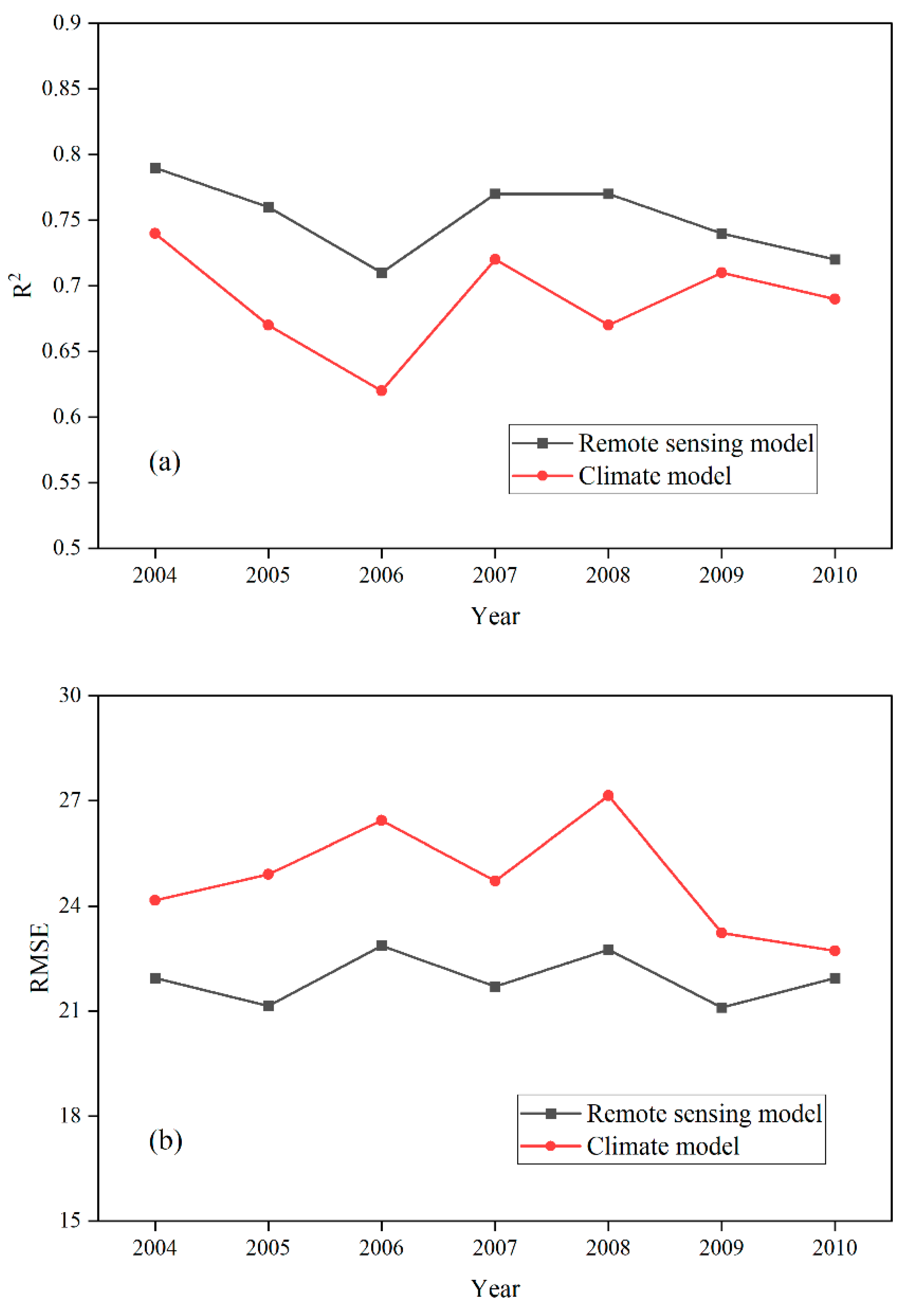
2.1.1. Comparison of the Remote Sensing Model and Climate Model

In this study, we tested the effect of remote sensing data and climate data on MSFD simulation at two timescales (i.e., decadal and annual scales). According to the different data sources used to build the model, we defined the predictors as two models, a full remote sensing model and a full climate model. The differences between the two sets of predictors were (1) the data sources of FDD, TDD and snow were different (detailed in Section 2.2), and (2) the LAI data representing vegetation were available in the remote sensing model but not in the climate model (Equations (1) and (2)).
MSFD = TDD (MODIS) + FDD (MODIS) + SCDs + LAI + Soil (6 properties) + DEM + SR + RP
MSFD = TDD (WC) + FDD (WC) + SP + LAI + Soil (6 properties) + DEM + SR + RP
where TDD (MODIS) and FDD (MODIS) represent the freezing and thawing degree days, respectively, based on MODIS surface temperature; TDD (WC) and FDD (WC) represent the freezing and thawing degree days, respectively, based on climate data; SCDs are snow cover days; SR is the solar radiation; SP is the snow precipitation; and RP is the rain precipitation.
To reduce the complexity of the model and remove the possible collinearity between variables, we simplified the model by using extremely randomized trees (Extra-Trees) in Python and established two kinds of simplified models, a simplified remote sensing model and a simplified climate model. This method calculated the Gini coefficient of each feature by selecting the optimal partition attribute to ensure the highest purity at the node. The feature_importances_ function returns the importance of each feature. A feature variable is more important the larger its value. According to the importance of variables, 8 predictors in the full remote sensing model and 7 predictors in the full climate model were used to build the simplified remote sensing model and climate model, respectively (Equations (3) and (4)).
MSFD = TDD (MODIS) + FDD (MODIS) + SCDs + LAI + Soil (bulk density) + DEM + SR + RP
MSFD = TDD (WC) + FDD (WC) + SCDs + SP + Soil (bulk density) + DEM + SR + RP

2.1.2. Statistical/Machine Learning Model

Four poplar statistical/machine learning techniques, random forest (RF), support vector regression (SVR), k-nearest neighbor (KNN), and ensemble average were used; three of the models were compared based on cross-validation.
RF is an ensemble learning algorithm based on decision trees developed by Breiman [53]. It uses bootstrap repetitive sampling and extracts samples from the total sample for modeling. The final output result is the average of the results of all decision trees [54]. In this study, the number of trees was set to 100, and the nodes of each tree were divided into random features and random thresholds. SVR establishes a regression model based on a given error interval (ε). If the simulated value falls within the error range, the predicted value is considered correct, and the kernel function directly determines the performance of the support vector machine. This study used the most commonly used kernel function, the radial basis kernel function [55], and the penalty parameter was set to 100. KNN found the k-nearest neighbors of each query point from the training sample and used the average of the k-nearest neighbors as the prediction target [56]. The value of k was set to 10, and the weights were assigned based on the distance from the target point to the k points in this study. The above three machine learning algorithms were all implemented using the scikit-learn module in Python [57].
Tenfold cross-validation was used to evaluate the predictive performance of each machine/statistical model. A total of 184 ground-measured SFD sample points were collected from 2001 to 2010 on the QTP. For each model, 165 sample points were used for model training, and the remaining 19 sample points were used for model validation. To reduce the uncertainty of the model, each model was run 200 times, and the arithmetic average was used as the final simulation accuracy. The root mean square error (RMSE), coefficient of determination (R2) and bias (mean difference) were used to evaluate the performance of the model.

2.1.3. Trainability of Statistical/Machine Learning Models

To assess the trainability of statistical/machine learning models to simulate the MSFD in the past, the trained model using the in situ MSFD data at the baseline period (2001–2010) was used to project the MSFD at two historical periods (1981–1990 and 1991–2000). We assumed the DEM, solar radiation and soil properties did not change on a long time scale, and the climate conditions in the historical periods, including the rain precipitation, snow precipitation, FDD and TDD, were adopted as the remaining inputs. The in situ MSFD measurement was used to validate the simulation accuracy and assess the accuracy change relative to the baseline period (2001–2010).

2.2. Data

2.2.1. MSFD Measurement Data

In this study, daily soil freezing depth measurement data from 184 meteorological stations on the QTP were collected from 1981 to 2010. First, we found the annual MSFD of each site in the daily data from 1981 to 2000. Then, the average MSFD of the three periods was calculated using the MSFD of ten years, i.e., 1981–1990, 1991–2000 and 2001–2010.
Due to the lack of data from some sites, the numbers of sites available in 1981–1990, 1991–2000, and 2001–2010 were 84, 89, and 184, respectively. MSFD measurement data in the baseline period (2001–2010) were used for model training and cross-validation, and observed MSFD in the historical periods (1981–1990 and 1991–2000) from all available sites were used to validate the performance of the model. The spatial distribution of the sites is shown in Figure 1. The altitude of these sites was 846–4800 m, and the MSFD was 3.7–276.6 cm. Among them, the average MSFD of the sites less than 100 cm, 100–200 cm, and greater than 200 cm accounted for 75.54, 22.28, and 2.74%, respectively.

2.2.2. Remotely Sensed Annual Freezing and Thawing Degree-Days

The multiyear average FDD and TDD were generated by calculating the 1 km resolution MODIS products (MOD11A1 and MYD11A1 v5) four times a day [58,59]. To obtain the complete daily average LST in time and space and reduce the error caused by missing data [60,61], a gap-filling scheme was adopted [62]. This scheme uses the pixels with complete data (i.e., four times LST data are available) to directly calculate the daily LST amplitude, and estimates the daily mean LST of the missing pixels (i.e., daytime or nighttime LST data is missing) using the amplitude. The specific details of the gap-filling method are presented in [47]. Based on the daily average LST, the FDD and TDD from 2001 to 2010 were calculated. The annual average FDD and TDD were used as predictors of the MSFD simulation to construct the remote sensing variable model.

2.2.3. Snow-Cover Days (SCDs)

The SCD product adopts the daily cloudless snow product in combination with MODIS daily snow products (MOD10A1, MYD10A1) and AMSR-E/Aqua snow water equivalent products in the middle and high latitude regions of Eurasia, with a spatial resolution of 500 m [63]. The validation results show that it is basically consistent with the daily cloudless snow product synthesized based on Landsat 5, and the kappa coefficient is 0.57 [50]. In this paper, the average annual snow cover days from 2001 to 2010 were calculated and resampled to 1 km. This predictor was used to construct the remote sensing variable model.

2.2.4. Leaf Area Index (LAI)

The LAI data adopt the 2001–2010 Global Land Surface Satellite (GLASS) product. The dataset uses a long-term series of MODIS and AVHRR reflectance data to generate GLASS LAI products from 1981 to 2012 year by year, based on the neural network method [64]. The validation results showed that GLASS LAI products had higher accuracy than did MODIS and CYCLOPES LAI products [65]. The LAI data were used to construct a remote sensing variable model.

2.2.5. Soil Data

Soil data were obtained using SoilGrids250m, which was developed by the International Soil Reference and Information Center (ISRIC—World Soil Information, Wageningen, the Netherlands) [66]. Based on the first version, the machine learning integrated algorithm was used to replace the original linear regression algorithm, the spatial resolution was increased from the original 1 km to 250 m, and the relative accuracy was increased from 60 to 230%. The data included soil organic carbon content (g kg−1), bulk density (kg m−3), coarse fragments (volumetric %), and silt, clay, and sand contents (weight %) at 7 depths (0, 5, 15, 30, 60, 100, and 200 cm). In this study, the thickness of 7 layers of soil was used as the weight, and the weighted average of each component of the soil was resampled to 1 km.

2.2.6. Digital Elevation Model (DEM)

The DEM data were obtained by the National Aeronautics and Space Administration (NASA) Shuttle Radar Topographic Mission (SRTM). The SRTM data are categorized into SRTM1 and SRTM3 according to the accuracy, and the corresponding spatial resolutions are 30 and 90 m, respectively. SRTM1 was used in this study and resampled to 1 km.

2.2.7. Downscaled Climate Data

The climate data including the monthly average temperature (°C), precipitation (mm) and solar radiation (kJ m−2 day−1) derived from WorldClim v2.1 (https://worldclim.org, accessed on 24 November 2021) with a spatial resolution of 1 km [67]. Except for the solar radiation data, the temporal resolution of the temperature and precipitation indicators (1970–2000) did not fit the time frame of this study (2001–2010). Therefore, following Ran et al. (2021), we adopted an adjustment scheme to obtain the temperature and precipitation data with a resolution of 1 km from 2001 to 2010. First, nearest-neighbor interpolation was used to resample the monthly average weather data of WorldClim from 2001 to 2010 (with a spatial resolution of 21 km2) to 1 km. Then, according to the local smoothing (3 × 3 window) difference of the resampled weather data, the temperature and precipitation data from 1970 to 2000 were adjusted to 2001–2010. The specific adjustment scheme refers to [48]. Finally, four predictors were calculated from the adjusted climate data, including the freezing and thawing index (the cumulative value of monthly average temperature above 0 °C and below 0 °C, respectively [68]), snow precipitation (precipitation sum in millimeters for months below 0 °C) and rain precipitation (precipitation sum for months above 0 °C). These predictors were used to construct a climate variable model.

2.2.8. Ancillary Data
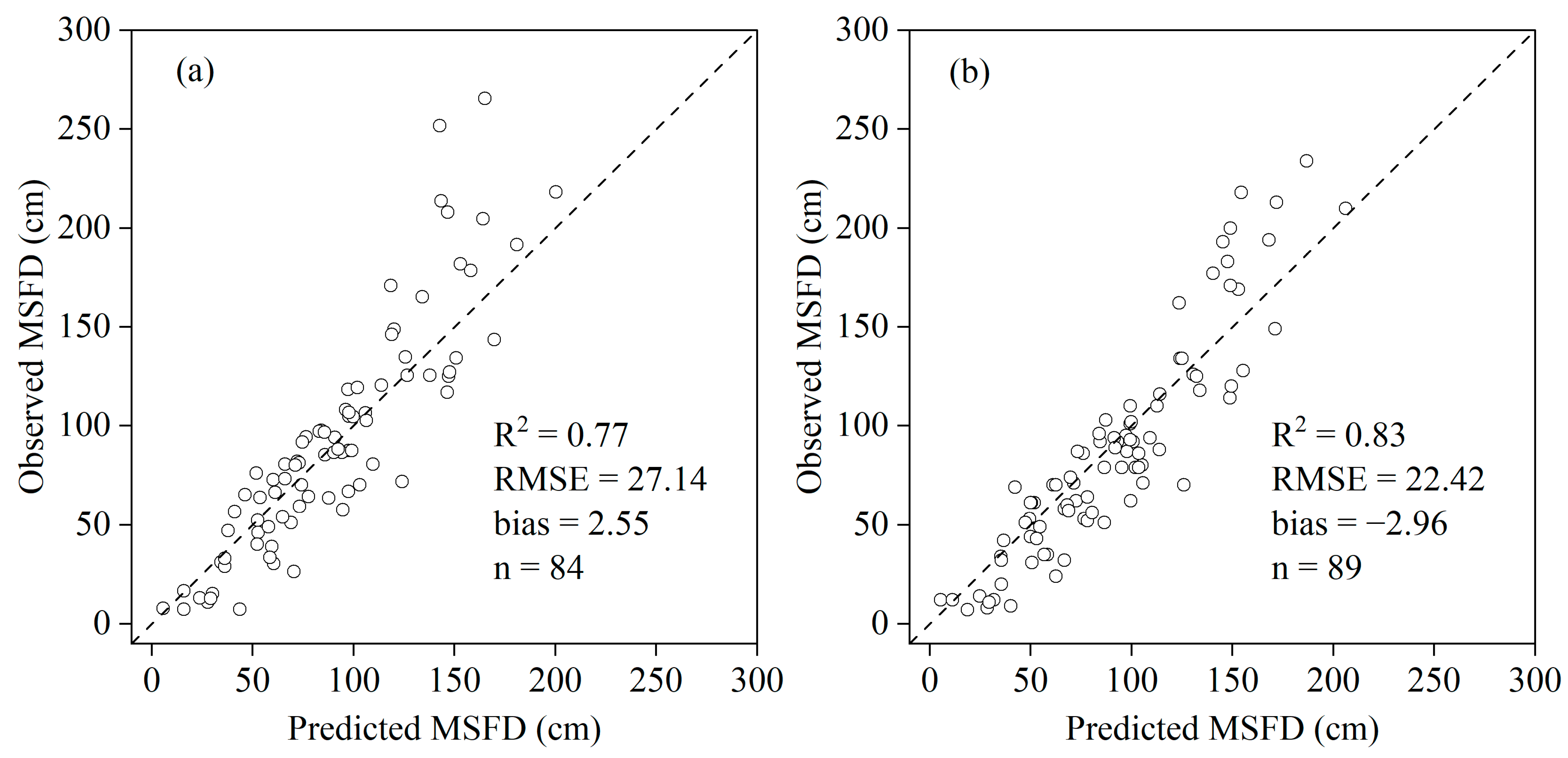
The permafrost, glaciers and lakes were excluded in the final simulated MSFD map. The permafrost area adopted the recently released high-precision 1km spatial resolution permafrost map [29]. Glacier extent used the Global Land Ice Measurement from the Space (GLIMS) geospatial glacier database [69], that could be downloaded at http://nsidc.org/glims/, accessed on 24 November 2021. The lake extent was derived from the levels 1 of the Global Lakes and Wetlands Database (GLWD) [70].

3. Results

3.1. The Comparison of Statistical/Machine Learning Model

RF, SVR, KNN and the ensemble averaging of the three models were used to construct the statistical/machine learning model, with remote sensing variables and climate variables as input conditions. Each model was run 200 times, and the results of 10-fold cross-validation (Table 1, Table 2, Table 3 and Table 4) showed that the results of the four models were not significantly different, but the SVR model was relatively good. The SVR model with the simplified remote sensing variables had better performance for the simulation of MSFD (R2 = 0.76, RMSE = 21.64 cm, bias = −1.22 cm). The simulation performance of SVR performed better than RF and KNN and was closest to the ensemble mean. The simulation accuracy of KNN showed obvious differences when full variables and simplified variables were used as input data. R2 increased by 0.11 and the RMSE decreased by 4.41 using KNN when simplified remote sensing variables were used as input conditions compared to the use of full climate variables. The RF algorithm was not very sensitive to input variables. Regardless of changing the amount of input data or the type of input variables, the difference in the R2 between them was less than 0.01, and the RMSE was less than 1 cm. The ensemble average of the three models could reduce the uncertainty and improve the accuracy of the simulation. KNN exhibited poor performance, which affected the performance of the ensemble mean when full variables were used as input conditions. However, the ensemble average of the three models was the best model when the accuracy of KNN was improved; for example, R2 was maximized and RMSE and bias were minimized compared with the other three models when simplified climate variables were used as input conditions. Therefore, the SVR algorithm had a strong spatial generalization ability and was more suitable for predicting the MSFD, which was consistent with the conclusion of [19].

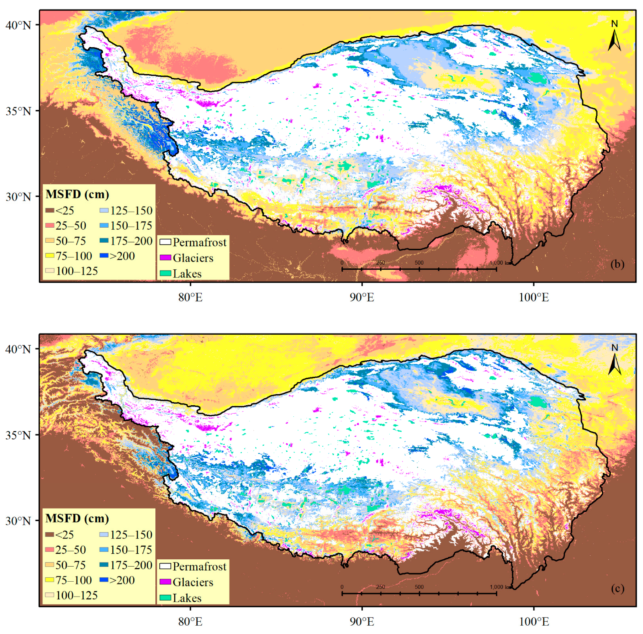
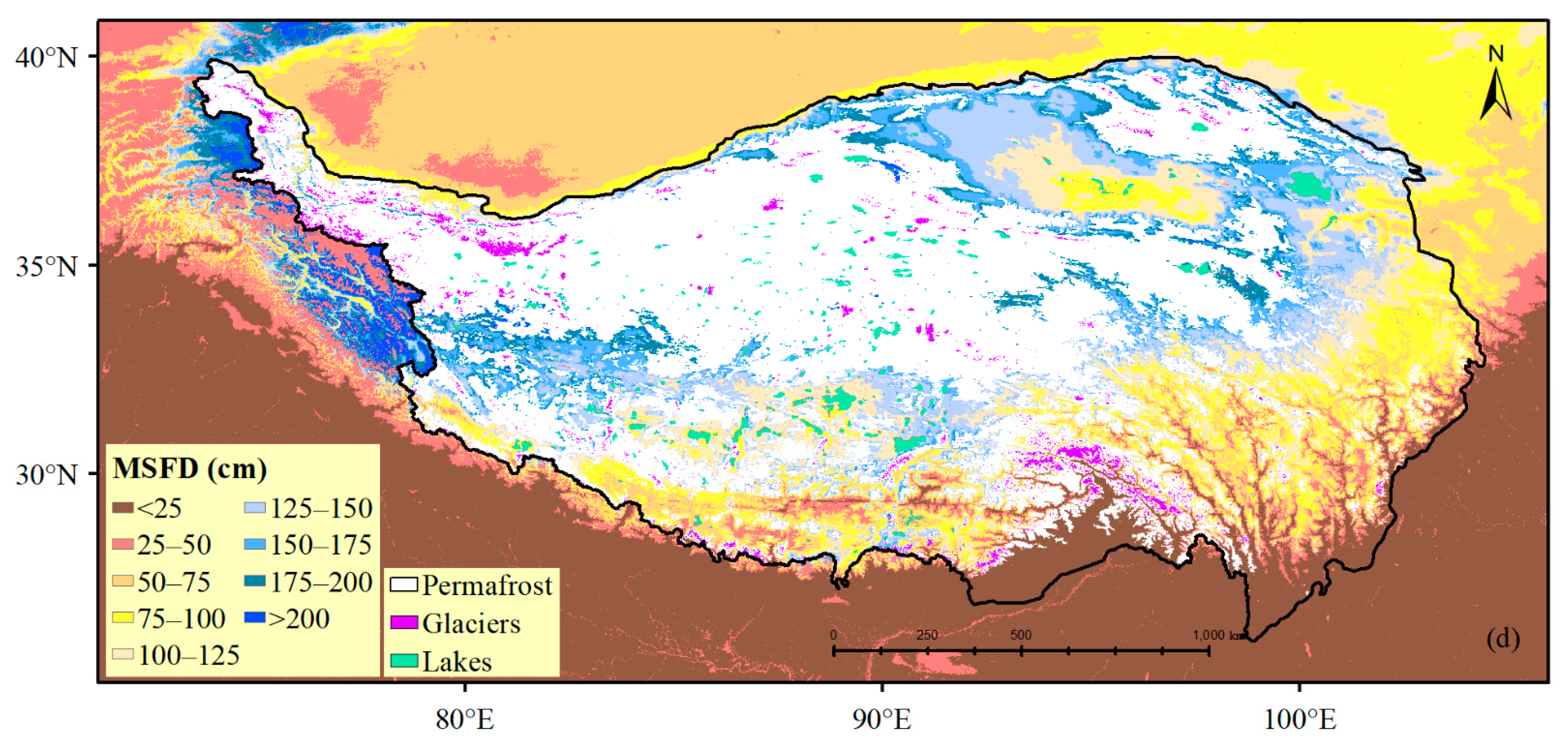
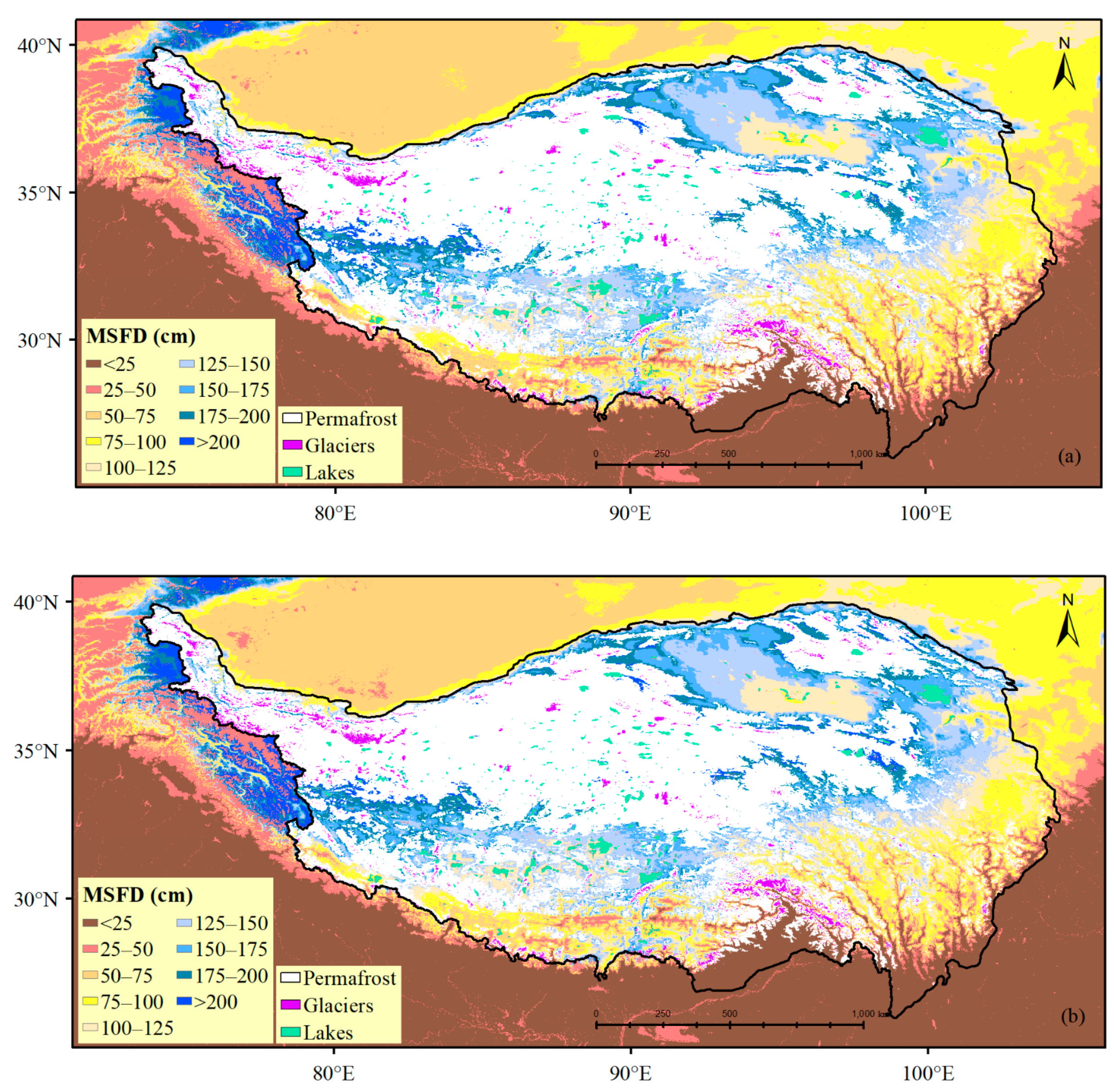
3.2. The Role of Remote Sensing Variables in Predicting the Change in MSFD

As mentioned in Section 3.1, cross-validation showed that SVR had the best simulation performance. Therefore, based on the four sets of predictive factors, SVR was used to map the average MSFD on the QTP from 2001 to 2010, excluding permafrost, glaciers and lakes (Figure 2). The remote sensing variables and the climate variables as different inputs of the SVR model showed differences in the performance of simulating the MSFD (p < 0.05, paired one-sided t-test, n = 200), and the simulation accuracy based on the remote sensing variables was higher than that of the climate variables. According to the cross-validation results (Table 1, Table 2, Table 3 and Table 4), compared with the climate variables, the R2 of the remote sensing variables was improved, and the RMSE was reduced, but the deviation was larger. For example, the R2 of the full remote sensing variables increased by 0.05, the RMSE decreased by 1.23 cm, the deviation increased by 1.57 cm; the R2 of the simplified remote sensing variables increased by 0.06, the RMSE decreased by 1.99 cm, and the deviation increased by 0.45 cm.
Regardless of whether the remote sensing variables or the climate variables were used, the accuracy of the simplified variables was improved. The R2 of the simplified remote sensing variables and the climate variables increased by 0.02 and 0.01, respectively, and the RMSE was reduced by 1.24 cm and 0.55 cm, respectively.
Spatially, using remote sensing variables for mapping the MSFD could show richer details, especially in the southern QTP, and the transition zone of the MSFD in the range of 25–100 cm was more obvious. This difference in detail might be related to the data richness of the FDD, and the FDD based on reanalysis data was calculated using monthly average temperatures that were interpolated using coarse-resolution weather data (spatial resolution of 5 km).
To test the effect of remote sensing data on the simulation of the MSFD at the annual scale, SVR with remote sensing variables and climate variables was constructed using the year-by-year observed MSFD from 2004 to 2010. According to the results of 200 simulations, the prediction indicators of the SVR model based on the simplified remote sensing variables and climate variables were calculated. The time series changes in the R2, RMSE and bias (Figure 3) showed that remote sensing observation data could improve the simulation accuracy of the MSFD on an annual time scale. The simulation performance index, i.e., the R2 value, of the remote sensing variables was always greater than that of the climate variable model, and the RMSE was always smaller than that of the climate variable model. The annual average R2 and RMSE based on the remote sensing variables were 0.75 and 21.92 cm, respectively, which increased by 0.08 and decreased by 2.84 cm compared with the annual average R2 based on the climate variables, respectively. The biases of the remote sensing variables and the climate variables from 2004 to 2010 were highly volatile; however, the multiyear average bias of the remote sensing variables was 0.02 cm smaller than that of the climate variables.
Both remote sensing variables and climate variables could be used to predict the MSFD; however, the DFF and LAI in remote sensing variables played an important role in the simulation, especially for the FDD data. The FDD in the climate variables was a form of indirectly expressing the thermal state of the MSFD because it was calculated based on the monthly average air temperature. There was a difference between air temperature and LST, and this difference might be related to vegetation types and climate background [28]. The FDD in remote sensing variables was the most direct environmental indicator affecting the MSFD, and it was calculated based on the daily average LST (i.e., the average of the four temperatures in a day). Therefore, remote sensing variables performed better as input.

3.3. The Transferability of the Current Model to Simulate Past Changes

The MSFD in the historical periods (1981–1990 and 1991–2000) was simulated using the SVR model trained in the baseline period (2001–2010) with simplified climate variables (Figure 4). We assumed that the conditions of soil properties, elevation and solar radiation were constant and changed the model input conditions of rain precipitation, snow precipitation, FDD and TDD for the corresponding periods. Eighty-nine observed MSFDs in the 1980s and 84 in the 1990s were used to validate the simulation results. The results showed that the predicted and observed values were in good agreement (Figure 5), which indicated that SVR with the simplified climate variables had good transferability. Compared with the 1990s (R2 = 0.83, RMSE = 22.42 cm), the simulation results for the 1980s (R2 = 0.77, RMSE = 27.14 cm) had a larger error, with an increase in the RMSE of 4.72 cm. Compared with the baseline period, the bias increased by 3.32 cm and 2.19 cm in the 1980s and 1990s, respectively, which suggested that the statistical/machine learning models had a time scale limitation in terms of reconstructing the spatial distribution of the past MSFD, and the uncertainty in the simulation increased with time from the baseline period. Therefore, prediction of the past and even the future MSFD could be achieved according to the method developed in this paper even if there were no environmental remote sensing variables related to the MSFD, e.g., land surface temperature, LAI.

4. Discussion

This study integrated the in situ measurement of the MSFD and spatial prediction factors to develop a data-driven model to simulate the current (2001–2010) and past (1981–1990 and 1991–2000) MSFD on the QTP. The accuracy of the models was supported by the metrics (i.e., R2, RMSE and bias) based on 10-fold cross-validation. The validation results showed that the SVR model had better spatial generalization ability and produced values closest to the multimodel ensemble mean. Previous studies reached similar conclusions showing that the SVR model performed better in data-driven simulations of frozen ground [19,47].
Input data were an important factor affecting data-driven prediction. Remote sensing data and climate data, as input conditions, have different advantages and roles in simulation. Snow cover, LAI and, especially, LST are used as the input conditions to effectively improve the simulation accuracy and are the key indicators used to reflect the thermal state of seasonally frozen ground [71,72]. Remote sensing data had high temporal and spatial resolution, which provided a good data source for studying the characteristics of MSFD changes at different time scales (i.e., decadal, annual and daily scales). In the case of a short time scale, the simulation accuracy of the MSFD might be higher. LST retrieval from thermal infrared remote sensing, LAI, and snow cover significantly contribute to the performance of the model. At the same time, the data obtained by different remote sensing technologies have potential as predictors to drive machine learning models. For example, soil moisture from microwave remote sensing has the potential to overcome the data challenge of MSFD simulation [31,34,35,73].
Climate data can be used as input conditions for the model when remote sensing variables are not available. We found that the model with climate variables had good transferability, which made it possible to simulate the MSFD when remote sensing data (FDD, TDD, snow cover and vegetation) were not available in the past or in the future. Many previous studies also used the transferability of the data-driven model to predict the mean annual ground temperature (MAGT) [48,74], active layer thickness (ALT) [48] and MSFD [19] in the past and future periods. However, the transferability of the model had a certain time-scale limitation; that is, when the frozen ground and climatic conditions reached a balance on a long-term scale [28], the accuracy of the simulation decreased with increasing distance from the baseline period, and the uncertainty increased due to the forgetfulness and error accumulation of the machine model [75].

5. Conclusions

In this study, we assessed the performance of data-driven models to simulate the MSFD on the QTP with different configurations of predictors for different periods. RF, SVR, KNN and the average of the three models with different input conditions (i.e., remote sensing variables and climate variables) were compared in the baseline period (2001–2010). We found that the SVR model was better for the simulation of MSFD than the RF, KNN, and multimodel mean models, regardless of whether they were driven by remote sensing or climate variables. The diversity of remote sensing-based variable inputs improved the estimation of seasonal maximum freezing depth relative to the reanalysis climate inputs, both on the decadal scale and on the annual scale. When remote sensing variables were not available, the climate data-driven machine learning model could be used to trace the past and predict the future MSFD, but its accuracy decreased with the extension of prediction periods.
In the future, data-driven MSFD simulation could be improved in at least two ways: input data and model structure. Multiple deep learning architectures, such as deep belief networks, recurrent neural networks, and convolutional neural networks, that have achieved great success in other fields might be promising to promote MSFD simulation. More remote sensing variables, such as downscaled microwave remote sensing products, and higher resolution optical remote sensing, such as Landsat data, have the potential to improve the accuracy and spatial resolution of MSFD simulations.

Author Contributions

B.W. and Y.R. contributed equally to the design, data processing, analysis, and manuscript writing. All authors have read and agreed to the published version of the manuscript.

Funding

This research was funded by the China National Natural Science Foundation (No. 42071421), National Science and Technology Major Project of China’s High Resolution Earth Observation System (Project Number: 21-Y20B01-9001-19/22).

Institutional Review Board Statement

Not applicable.

Informed Consent Statement

Not applicable.

Data Availability Statement

The data presented in this study are available on request from the corresponding author.

Acknowledgments

The authors are grateful to the editors and anonymous reviewers for their insightful comments and suggestions that helped improve this paper.

Conflicts of Interest

The authors declare no conflict of interest.

References

  1. Huggel, C.; Salzmann, N.; Allen, S.; Caplan-Auerbach, J.; Fischer, L.; Haeberli, W.; Larsen, C.; Schneider, D.; Wessels, R. Recent and future warm extreme events and high-mountain slope stability. Philos. Trans. R. Soc. A Math. Phys. Eng. Sci. 2010, 368, 2435–2459. [Google Scholar] [CrossRef] [Green Version]
  2. Evans, S.G.; Ge, S. Contrasting hydrogeologic responses to warming in permafrost and seasonally frozen ground hillslopes. Geophys. Res. Lett. 2017, 44, 1803–1813. [Google Scholar] [CrossRef]
  3. Frauenfeld, O.W.; Zhang, T. An observational 71-year history of seasonally frozen ground changes in the Eurasian high latitudes. Environ. Res. Lett. 2011, 6, 044024. [Google Scholar] [CrossRef] [Green Version]
  4. Cuo, L.; Zhang, Y.; Bohn, T.J.; Zhao, L.; Li, J.; Liu, Q.; Zhou, B. Frozen soil degradation and its effects on surface hydrology in the northern Tibetan Plateau. J. Geophys. Res. Atmos. 2015, 120, 8276–8298. [Google Scholar] [CrossRef] [Green Version]
  5. Qiu, J. China: The Third Pole. Nat. News 2008, 454, 393–396. [Google Scholar] [CrossRef] [Green Version]
  6. Chang, Y.; Lyu, S.; Luo, S.; Li, Z.; Fang, X.; Chen, B.; Li, R.; Chen, S. Estimation of permafrost on the Tibetan Plateau under current and future climate conditions using the CMIP5 data. Int. J. Clim. 2018, 38, 5659–5676. [Google Scholar] [CrossRef]
  7. Shi, Y.; Niu, F.; Yang, C.; Che, T.; Lin, Z.; Luo, J. Permafrost Presence/Absence Mapping of the Qinghai-Tibet Plateau Based on Multi-Source Remote Sensing Data. Remote Sens. 2018, 10, 309. [Google Scholar] [CrossRef] [Green Version]
  8. Wang, J.; Luo, S.; Li, Z.; Wang, S.; Li, Z. The freeze/thaw process and the surface energy budget of the seasonally frozen ground in the source region of the Yellow River. Theor. Appl. Clim. 2019, 138, 1631–1646. [Google Scholar] [CrossRef] [Green Version]
  9. Luo, S.; Fang, X.; Lyu, S.; Jiang, Q.; Wang, J. Interdecadal Changes in the Freeze Depth and Period of Frozen Soil on the Three Rivers Source Region in China from 1960 to 2014. Adv. Meteorol. 2017, 2017, 1–14. [Google Scholar] [CrossRef] [Green Version]
  10. Wang, R.; Dong, Z.; Zhou, Z. Effect of decreasing soil frozen depth on vegetation growth in the source region of the Yellow River for 1982–2015. Theor. Appl. Clim. 2020, 140, 1185–1197. [Google Scholar] [CrossRef]
  11. Boli, C.; Siqiong, L.; Shihua, L.; Yu, Z.; Di, M. Effects of the soil freeze-thaw process on the regional climate of the Qinghai-Tibet Plateau. Clim. Res. 2014, 59, 243–257. [Google Scholar] [CrossRef]
  12. Christensen, A.F.; He, H.; Dyck, M.F.; Turner, E.L.; Chanasyk, D.S.; Naeth, M.A.; Nichol, C. In situ measurement of snowmelt infiltration under various topsoil cap thicknesses on a reclaimed site. Can. J. Soil Sci. 2013, 93, 497–510. [Google Scholar] [CrossRef] [Green Version]
  13. Jafarov, E.; Schaefer, K. The importance of a surface organic layer in simulating permafrost thermal and carbon dynamics. Cryosphere 2016, 10, 465–475. [Google Scholar] [CrossRef] [Green Version]
  14. Luo, S.; Chen, B.; Lyu, S.; Fang, X.; Wang, J.; Meng, X.; Shang, L.; Wang, S.; Ma, D. An Improvement of Soil Temperature Simulations on the Tibetan Plateau. Sci. Cold Arid Reg. 2018, 10, 80–94. [Google Scholar]
  15. Mu, C.; Zhang, T.; Wu, Q.; Cao, B.; Zhang, X.; Peng, X.; Wan, X.; Zheng, L.; Wang, Q.; Cheng, G. Carbon and Nitrogen Properties of Permafrost over the Eboling Mountain in the Upper Reach of Heihe River Basin, Northwestern China. Arct. Antarct. Alp. Res. 2015, 47, 203–211. [Google Scholar] [CrossRef] [Green Version]
  16. Shiklomanov, N.I.; Nelson, F.E. Active-layer mapping at regional scales: A 13-year spatial time series for the Kuparuk region, north-central Alaska. Permafr. Periglac. Process. 2002, 13, 219–230. [Google Scholar] [CrossRef]
  17. Yanai, Y.; Iwata, Y.; Hirota, T. Optimum soil frost depth to alleviate climate change effects in cold region agriculture. Sci. Rep. 2017, 7, 44860. [Google Scholar] [CrossRef] [Green Version]
  18. Shugar, D.H.; Jacquemart, M.; Shean, D.; Bhushan, S.; Upadhyay, K.; Sattar, A.; Schwanghart, W.; McBride, S.; Vries, M.V.W.d.; Mergili, M.; et al. A massive rock and ice avalanche caused the 2021 disaster at Chamoli, Indian Himalaya. Science 2021, 373, 300–306. [Google Scholar] [CrossRef]
  19. Wang, T.; Yang, D.; Fang, B.; Yang, W.; Qin, Y.; Wang, Y. Data-driven mapping of the spatial distribution and potential changes of frozen ground over the Tibetan Plateau. Sci. Total Environ. 2018, 649, 515–525. [Google Scholar] [CrossRef]
  20. Liu, L.; Luo, D.; Wang, L.; Huang, Y.; Chen, F. Variability of soil freeze depth in association with climate change from 1901 to 2016 in the upper Brahmaputra River Basin, Tibetan Plateau. Theor. Appl. Clim. 2020, 142, 19–28. [Google Scholar] [CrossRef]
  21. Peng, X.; Zhang, T.; Frauenfeld, O.W.; Wang, K.; Cao, B.; Zhong, X.; Su, H.; Mu, C. Response of seasonal soil freeze depth to climate change across China. Cryosphere 2017, 11, 1059–1073. [Google Scholar] [CrossRef] [Green Version]
  22. Qin, Y.; Chen, J.; Yang, D.; Wang, T. Estimating Seasonally Frozen Ground Depth From Historical Climate Data and Site Measurements Using a Bayesian Model. Water Resour. Res. 2018, 54, 4361–4375. [Google Scholar] [CrossRef]
  23. Li, X.; Koike, T. Frozen soil parameterization in SiB2 and its validation with GAME-Tibet observations. Cold Reg. Sci. Technol. 2003, 36, 165–182. [Google Scholar] [CrossRef]
  24. Gouttevin, I.; Krinner, G.; Ciais, P.; Polcher, J.; Legout, C. Multi-scale validation of a new soil freezing scheme for a land-surface model with physically-based hydrology. Cryosphere 2012, 6, 407–430. [Google Scholar] [CrossRef] [Green Version]
  25. Rawlins, M.A.; Nicolsky, D.J.; McDonald, K.C.; Romanovsky, V.E. Simulating soil freeze/thaw dynamics with an improved pan-Arctic water balance model. J. Adv. Model. Earth Syst. 2013, 5, 659–675. [Google Scholar] [CrossRef]
  26. Zhang, Y.; Cheng, G.; Li, X.; Jin, H.; Yang, D.; Flerchinger, G.N.; Chang, X.; Bense, V.F.; Han, X.; Liang, J. Influences of Frozen Ground and Climate Change on Hydrological Processes in an Alpine Watershed: A Case Study in the Upstream Area of the Hei’he River, Northwest China. Permafr. Periglac. Process. 2016, 28, 420–432. [Google Scholar] [CrossRef]
  27. Walvoord, M.A.; Kurylyk, B.L. Hydrologic Impacts of Thawing Permafrost-A Review. Vadose Zone J. 2016, 15, 1–20. [Google Scholar] [CrossRef]
  28. Ran, Y.; Li, X. Progress, Chanllenges and opportunities of permafrost mapping in China. Adv. Earth Sci. 2019, 34, 1015–1027. [Google Scholar] [CrossRef]
  29. Ran, Y.; Li, X.; Cheng, G.; Che, J.; Aalto, J.; Karjalainen, O.; Hjort, J.; Luoto, M.; Jin, H.; Obu, J.; et al. New High-Resolution Estimates of the Permafrost Thermal State and Hydrothermal Conditions over the Northern Hemisphere. Earth Syst. Sci. Data Discuss. 2021, 2021, 1–27. [Google Scholar] [CrossRef]
  30. McDonald, K.C.; Kimball, J.S. Estimation of Surface Freeze-Thaw States Using Microwave Sensors. In Encyclopedia of Hydrological Sciences; Anderson, M.G., McDonnell, J.J., Eds.; John Wiley & Sons, Ltd.: Chichester, UK, 2005; p. has 059a. ISBN 978-0-471-49103-3. [Google Scholar]
  31. Park, S.-E. Variations of Microwave Scattering Properties by Seasonal Freeze/Thaw Transition in the Permafrost Active Layer Observed by ALOS PALSAR Polarimetric Data. Remote Sens. 2015, 7, 17135–17148. [Google Scholar] [CrossRef] [Green Version]
  32. Park, S.-E.; Bartsch, A.; Sabel, D.; Wagner, W.; Naeimi, V.; Yamaguchi, Y. Monitoring freeze/thaw cycles using ENVISAT ASAR Global Mode. Remote Sens. Environ. 2011, 115, 3457–3467. [Google Scholar] [CrossRef]
  33. Kostadinov, T.S.; Schumer, R.; Hausner, M.; Bormann, K.J.; Gaffney, R.; McGwire, K.; Painter, T.H.; Tyler, S.; Harpold, A.A. Watershed-scale mapping of fractional snow cover under conifer forest canopy using lidar. Remote Sens. Environ. 2018, 222, 34–49. [Google Scholar] [CrossRef]
  34. Zhao, T.; Shi, J.; Hu, T.; Zhao, L.; Zou, D.; Wang, T.; Ji, D.; Li, R.; Wang, P. Estimation of high-resolution near-surface freeze/thaw state by the integration of microwave and thermal infrared remote sensing data on the Tibetan Plateau. Earth Space Sci. 2017, 4, 472–484. [Google Scholar] [CrossRef]
  35. Hu, T.; Zhao, T.; Zhao, K.; Shi, J. A continuous global record of near-surface soil freeze/thaw status from AMSR-E and AMSR2 data. Int. J. Remote Sens. 2019, 40, 6993–7016. [Google Scholar] [CrossRef]
  36. Hansen, M.C.; Potapov, P.V.; Moore, R.; Hancher, M.; Turubanova, S.A.; Tyukavina, A.; Thau, D.; Stehman, S.V.; Goetz, S.J.; Loveland, T.R.; et al. High-resolution global maps of 21st-century forest cover change. Science 2013, 342, 850–853. [Google Scholar] [CrossRef] [Green Version]
  37. Kostadinov, T.S.; Lookingbill, T.R. Snow cover variability in a forest ecotone of the Oregon Cascades via MODIS Terra products. Remote Sens. Environ. 2015, 164, 155–169. [Google Scholar] [CrossRef] [Green Version]
  38. Muhuri, A.; Gascoin, S.; Menzel, L.; Kostadinov, T.S.; Harpold, A.A.; Sanmiguel-Vallelado, A.; Moreno, J.I.L. Performance Assessment of Optical Satellite-Based Operational Snow Cover Monitoring Algorithms in Forested Landscapes. IEEE J. Sel. Top. Appl. Earth Obs. Remote Sens. 2021, 14, 7159–7178. [Google Scholar] [CrossRef]
  39. Hall, D.K.; Kelly, R.; Riggs, G.A.; Chang, A.T.C.; Foster, J.L. Assessment of the relative accuracy of hemispheric-scale snow-cover maps. Ann. Glaciol. 2002, 34, 24–30. [Google Scholar] [CrossRef] [Green Version]
  40. Jin, M.; Dickinson, R.E. Land surface skin temperature climatology: Benefitting from the strengths of satellite observations. Environ. Res. Lett. 2010, 5, 5. [Google Scholar] [CrossRef] [Green Version]
  41. Pepin, N.C.; Maeda, E.E.; Williams, R. Use of remotely sensed land surface temperature as a proxy for air temperatures at high elevations: Findings from a 5000 m elevational transect across Kilimanjaro. J. Geophys. Res. Atmos. 2016, 121, 9998–10015. [Google Scholar] [CrossRef] [Green Version]
  42. Vancutsem, C.; Ceccato, P.; Dinku, T.; Connor, S.J. Evaluation of MODIS land surface temperature data to estimate air temperature in different ecosystems over Africa. Remote Sens. Environ. 2010, 114, 449–465. [Google Scholar] [CrossRef]
  43. Hachem, S.; Duguay, C.R.; Allard, M. Comparison of MODIS-derived land surface temperatures with ground surface and air temperature measurements in continuous permafrost terrain. Cryosphere 2012, 6, 51–69. [Google Scholar] [CrossRef] [Green Version]
  44. Zhu, W.; Lű, A.; Jia, S. Estimation of daily maximum and minimum air temperature using MODIS land surface temperature products. Remote Sens. Environ. 2013, 130, 62–73. [Google Scholar] [CrossRef]
  45. Jin, M.; Dickinson, R.E.; Vogelmann, A. A Comparison of CCM2–BATS Skin Temperature and Surface-Air Temperature with Satellite and Surface Observations. J. Clim. 1997, 10, 1505–1524. [Google Scholar] [CrossRef]
  46. Obu, J.; Westermann, S.; Bartsch, A.; Berdnikov, N.; Christiansen, H.H.; Dashtseren, A.; Delaloye, R.; Elberling, B.; Etzelmüller, B.; Kholodov, A.; et al. Northern Hemisphere permafrost map based on TTOP modelling for 2000–2016 at 1 km2 scale. Earth-Sci. Rev. 2019, 193, 299–316. [Google Scholar] [CrossRef]
  47. Ran, Y.; Li, X.; Cheng, G.; Nan, Z.; Che, J.; Sheng, Y.; Wu, Q.; Jin, H.; Luo, D.; Tang, Z.; et al. Mapping the permafrost stability on the Tibetan Plateau for 2005–2015. Sci. China Earth Sci. 2020, 64, 62–79. [Google Scholar] [CrossRef]
  48. Aalto, J.; Karjalainen, O.; Hjort, J.; Luoto, M. Statistical Forecasting of Current and Future Circum-Arctic Ground Temperatures and Active Layer Thickness. Geophys. Res. Lett. 2018, 45, 4889–4898. [Google Scholar] [CrossRef] [Green Version]
  49. Nelson, F.E.; Outcalt, S.I. A Computational Method for Prediction and Regionalization of Permafrost. Arct. Alp. Res. 1987, 19, 279. [Google Scholar] [CrossRef]
  50. Wang, Y.; Huang, X.; Liang, H.; Sun, Y.; Feng, Q.; Liang, T. Tracking Snow Variations in the Northern Hemisphere Using Multi-Source Remote Sensing Data (2000–2015). Remote Sens. 2018, 10, 136. [Google Scholar] [CrossRef] [Green Version]
  51. Zhang, T. Influence of the seasonal snow cover on the ground thermal regime: An overview. Rev. Geophys. 2005, 43, RG4002. [Google Scholar] [CrossRef]
  52. Ala-Aho, P.; Autio, A.; Bhattacharjee, J.; Isokangas, E.; Kujala, K.; Marttila, H.; Menberu, M.; Meriö, L.-J.; Postila, H.; Rauhala, A.; et al. What conditions favor the influence of seasonally frozen ground on hydrological partitioning? A systematic review. Environ. Res. Lett. 2021, 16, 043008. [Google Scholar] [CrossRef]
  53. Breiman, L. Random Forests. Mach. Learn. 2001, 45, 5–32. [Google Scholar] [CrossRef] [Green Version]
  54. Peters, J.; De Baets, B.; Verhoest, N.; Samson, R.; Degroeve, S.; De Becker, P.; Huybrechts, W. Random forests as a tool for ecohydrological distribution modelling. Ecol. Model. 2007, 207, 304–318. [Google Scholar] [CrossRef]
  55. Deluigi, N.; Lambiel, C.; Kanevski, M. Data-driven mapping of the potential mountain permafrost distribution. Sci. Total Environ. 2017, 590-591, 370–380. [Google Scholar] [CrossRef] [Green Version]
  56. Zhang, M.-L.; Zhou, Z.-H. ML-KNN: A lazy learning approach to multi-label learning. Pattern Recognit. 2007, 40, 2038–2048. [Google Scholar] [CrossRef] [Green Version]
  57. Pedregosa, F.; Varoquaux, G.; Gramfort, A.; Michel, V.; Thirion, B.; Grisel, O.; Blondel, M.; Prettenhofer, P.; Weiss, R.; Dubourg, V. Scikit-Learn: Machine Learning in Python. J. Mach. Learn. Res. 2011, 12, 2825–2830. [Google Scholar]
  58. Wan, Z. New refinements and validation of the collection-6 MODIS land-surface temperature/emissivity product. Remote Sens. Environ. 2014, 140, 36–45. [Google Scholar] [CrossRef]
  59. Wan, Z.; Zhang, Y.; Zhang, Q.; Li, Z.-L. Validation of the land-surface temperature products retrieved from Terra Moderate Resolution Imaging Spectroradiometer data. Remote Sens. Environ. 2002, 83, 163–180. [Google Scholar] [CrossRef]
  60. Soliman, A.; Duguay, C.; Saunders, W.; Hachem, S. Pan-Arctic Land Surface Temperature from MODIS and AATSR: Product Development and Intercomparison. Remote Sens. 2012, 4, 3833–3856. [Google Scholar] [CrossRef] [Green Version]
  61. Westermann, S.; Langer, M.; Boike, J. Systematic bias of average winter-time land surface temperatures inferred from MODIS at a site on Svalbard, Norway. Remote Sens. Environ. 2012, 118, 162–167. [Google Scholar] [CrossRef] [Green Version]
  62. Garcia, D. Robust smoothing of gridded data in one and higher dimensions with missing values. Comput. Stat. Data Anal. 2009, 54, 1167–1178. [Google Scholar] [CrossRef] [Green Version]
  63. Wang, Y.; Huang, X.; Deng, J.; Ma, X.; Liang, T. Development and Validation for Daily Cloud -free Snow Products in Middle-and-high Latitude Areas in Eurasia. Remote Sens. Technol. Appl. 2016, 31, 1013–1021. [Google Scholar]
  64. Xiao, Z.; Liang, S.; Wang, J.; Chen, P.; Yin, X.; Zhang, L.; Song, J. Use of General Regression Neural Networks for Generating the GLASS Leaf Area Index Product From Time-Series MODIS Surface Reflectance. IEEE Trans. Geosci. Remote Sens. 2013, 52, 209–223. [Google Scholar] [CrossRef]
  65. Xiang, Y.; Xiao, Z.Q.; Liang, S.; Wang, J.D.; Song, J.L. Validation of Global LAnd Surface Satellite (GLASS) Leaf Area Index Product. J. Remote Sens. 2014, 18, 573–596. [Google Scholar]
  66. Hengl, T.; De Jesus, J.M.; Heuvelink, G.B.M.; Gonzalez, M.R.; Kilibarda, M.; Blagotić, A.; Shangguan, W.; Wright, M.N.; Geng, X.; Bauer-Marschallinger, B.; et al. SoilGrids250m: Global gridded soil information based on machine learning. PLoS ONE 2017, 12, e0169748. [Google Scholar] [CrossRef] [PubMed] [Green Version]
  67. Fick, S.E.; Hijmans, R.J. WorldClim 2: New 1-km spatial resolution climate surfaces for global land areas. Int. J. Climatol. 2017, 37, 4302–4315. [Google Scholar] [CrossRef]
  68. Westermann, S.; Østby, T.I.; Gisnås, K.; Schuler, T.V.; Etzelmüller, B. A ground temperature map of the North Atlantic permafrost region based on remote sensing and reanalysis data. Cryosphere 2015, 9, 1303–1319. [Google Scholar] [CrossRef] [Green Version]
  69. Raup, B.; Racoviteanu, A.; Khalsa, S.J.; Helm, C.; Armstrong, R.; Arnaud, Y. The GLIMS geospatial glacier database: A new tool for studying glacier change. Glob. Planet. Chang. 2007, 56, 101–110. [Google Scholar] [CrossRef]
  70. Lehner, B.; Döll, P. Development and validation of a global database of lakes, reservoirs and wetlands. J. Hydrol. 2004, 296, 1–22. [Google Scholar] [CrossRef]
  71. Luo, D.; Liu, L.; Jin, H.; Wang, X.; Chen, F. Characteristics of ground surface temperature at Chalaping in the Source Area of the Yellow River, northeastern Tibetan Plateau. Agric. For. Meteorol. 2019, 281, 107819. [Google Scholar] [CrossRef]
  72. Luo, D.; Jin, H.; Marchenko, S.S.; Romanovsky, V.E. Difference between near-surface air, land surface and ground surface temperatures and their influences on the frozen ground on the Qinghai-Tibet Plateau. Geoderma 2018, 312, 74–85. [Google Scholar] [CrossRef]
  73. Li, X.; Che, T.; Li, X.; Wang, L.; Duan, A.; Shangguan, D.; Pan, X.; Fang, M.; Bao, Q. CASEarth Poles: Big Data for the Three Poles. Bull. Am. Meteorol. Soc. 2020, 101, E1475–E1491. [Google Scholar] [CrossRef] [Green Version]
  74. Karjalainen, O.; Aalto, J.; Luoto, M.; Westermann, S.; Romanovsky, V.E.; Nelson, F.E.; Etzelmüller, B.; Hjort, J. Circumpolar permafrost maps and geohazard indices for near-future infrastructure risk assessments. Sci. Data 2019, 6, 190037. [Google Scholar] [CrossRef] [PubMed] [Green Version]
  75. Bontempi, G.; Taieb, S.B.; Le Borgne, Y.-A. Machine Learning Strategies for Time Series Forecasting. In European Business Intelligence Summer School; Springer, Berlin/Heidelberg, Germany, 2012; pp. 62–77. [Google Scholar]
Figure 1. Study area and spatial distribution of ground-based observation points.
Remotesensing 13 04829 g001
Figure 2. Spatial distribution of simulated MSFD using the SVR model for the baseline period (2001–2010). (a) Full remote sensing variables; (b) full climate variables; (c) simplified remote sensing variables; and (d) simplified climate variables.
Remotesensing 13 04829 g002aRemotesensing 13 04829 g002bRemotesensing 13 04829 g002c
Figure 3. Comparison of simulation performance between SVR with simplified remote sensing variables and SVR with climate variables for long time series. (a) Changes in squared correlations (R2) for different sets of variables from 2004 to 2010; (b) changes in the RMSE for different sets of variables from 2004 to 2010; and (c) changes in the bias for different sets of variables from 2004 to 2010.
Remotesensing 13 04829 g003aRemotesensing 13 04829 g003b
Figure 4. Spatial distribution of the MSFD in the past periods. (a) 1981–1990; (b) 1991–2000.
Remotesensing 13 04829 g004
Figure 5. The agreement between the observed and predicted values of the annual average MSFD in the past period based on the SVR model. The dashed black line indicates 1:1. (a) 1981–1990; (b) 1991–2000.
Remotesensing 13 04829 g005
Table 1. Simulation performance of the full remote sensing model.
RFSVRKNNEnsemble Mean
R20.65 ± 0.230.74 ± 0.140.57 ± 0.210.70 ± 0.18
RMSE26.10 ± 8.9022.86 ± 7.2329.28 ± 7.7324.33 ± 7.94
bias0.30 ± 6.28−2.20 ± 5.362.89 ± 6.690.33 ± 5.71
Table 2. Simulation performance of the full climate model.
RFSVRKNNEnsemble Mean
R20.66 ± 0.230.69 ± 0.290.60 ± 0.220.69 ± 0.22
RMSE25.55 ± 9.1124.09 ± 10.3828.27 ± 7.7524.47 ± 8.97
bias0.68 ± 6.01−0.63 ± 6.122.54 ± 6.390.86 ± 5.81
Table 3. Simulation performance of the simplified remote sensing model.
RFSVRKNNEnsemble Mean
R20.66 ± 0.230.76 ± 0.130.66 ± 0.200.73 ± 0.16
RMSE25.70 ± 8.8821.64 ± 6.8225.88 ± 7.9222.88 ± 7.80
bias0.48 ± 6.12−1.22 ± 5.092.49 ± 6.010.58 ± 5.42
Table 4. Simulation performance of the simplified climate model.
RFSVRKNNEnsemble Mean
R20.67 ± 0.230.70 ± 0.290.70 ± 0.230.72 ± 0.24
RMSE25.31 ± 9.1823.63 ± 10.3023.96 ± 8.9023.09 ± 9.39
bias0.81 ± 5.95−0.77 ± 6.011.41 ± 5.690.48 ± 5.89
Publisher’s Note: MDPI stays neutral with regard to jurisdictional claims in published maps and institutional affiliations.

