Study of the Boundary Layer Structure of a Landfalling Typhoon Based on the Observation from Multiple Ground-Based Doppler Wind Lidars

Abstract

The boundary layer structure is crucial to the formation and intensification of typhoons, but there is still a lack of high-precision turbulence observations in the typhoon boundary layer due to limitations of the observing instruments under typhoon conditions. Using joint observations from multiple ground-based Doppler wind lidars (DWL) collected by the Shanghai Typhoon Institute of China Meteorological Administration (CMA) during the transit of Typhoon Lekima (8–11 August 2019), the characteristics of the wind field and physical quantities (including turbulent kinetic energy (TKE) and typhoon boundary layer height (TBLH)) of the boundary layer of typhoon Lekima were analyzed. The magnitude of TKE was shown to be related not only to the horizontal wind speed but also to the presence of a strong downdraft, which leads to a rapid increase of TKE. The magnitudes of TKE in different quadrants of Typhoon Lekima were also found to differ. The TKE in the front right quadrant of the typhoon was 2.5–6.0 times that in the rear left quadrant and ~1.7 times that in the rear right quadrant. The TKE over the island was larger than that over the urban area. Before Typhoon Lekima made landfall, the TKE increased with decreasing distance to the typhoon center. After typhoon landfall, the TKE changes were different on the left and right sides of the typhoon center, with the TKE on the left decreasing rapidly, while that on the right changed little. The typhoon boundary layer height calculated by five methods was compared and was found to decrease gradually before typhoon landfall and increased gradually afterward. The trends of the TBLH calculated using helicity and TKE were consistent, and both determine the TBLH well, while the maximum tangential wind speed height (h_umax) was larger than the height calculated by other methods. This study confirms that DWL has a strong detecting capability for the finescale structure of the typhoon boundary layer and provides a powerful tool for the validation of numerical simulations of typhoon structure.

1. Introduction

The boundary layer regulates the radial and vertical distribution of enthalpy and momentum that is closely related to typhoon generation and intensification [1,2,3]. Numerous studies have shown that the typhoon boundary layer (TBL) plays a key role in the simulation of typhoon intensity and structure [4,5,6].

A critical element in many boundary layer parameterization schemes used in typhoon numerical models is the determination of the boundary layer height (BLH), as BLH is a key variable that regulates the vertical distribution of turbulent fluxes and helps to determine where the turbulent fluxes are negligible [7,8]. There is no consensus on how to define the typhoon BLH (TBLH), although it is a key parameter in numerical models. In the slab model used in the seminal theoretical hurricane model of Emanuel [9], the BLH is defined as a constant value. In early studies, Powell [10] and Anthes and Chang [11] adopted a BLH defined by thermodynamics; that is, the height where the rate of change of virtual potential temperature is zero. Bryan and Rotunno [12] defined the top of the boundary layer as the height of maximum wind, usually around 1 km. Smith et al. [13] adopted a dynamical definition, which considered the strong inflow layer as the BLH. In numerical models where turbulent fluxes are parameterized by a first-order K-profile method, the BLH is usually defined as the height at which the bulk Richardson number (Ri) reaches a threshold value (usually 0.25), where Ri is defined as the ratio of buoyancy to shear forcing [14]. Using these methods of calculating the TBLH, Kepert et al. [15] concluded that turbulence is mainly generated by shear, so the BLH is determined dynamically rather than thermodynamically, and the thermodynamic definition is not applicable to the hurricane boundary layer. Zhang et al. [16] evaluated three methods for calculating tropical cyclone BLH using data from 794 GPS dropsondes: two dynamical methods, (i) the height of the maximum wind speed and (ii) the inflow layer depth; and a thermodynamical method, the mixed layer depth. The BLH calculated using the thermodynamics is much smaller than those calculated from the dynamics. They also found that the method based on Ri does not accurately represent the BLH. Engeln [17] also argued that the traditional critical Ri only represents local turbulence and cannot properly characterize the turbulent properties of convective boundary layers.

Helicity is an important parameter in the study of flow characteristics in fluid dynamics [18,19]. Under typhoon conditions, Bogner et al. [20] calculated the total cell-relative helicity using dropsonde data and found that the cell-relative total helicity was inversely proportional to the distance from the hurricane center. Molinari et al. (2008) [21] discussed the distribution of helicity in Hurricane Bonnie (1998) and found large values of helicity in the boundary layer. Molinari et al. (2010) [22] pointed out that there are also large helicity values in the hurricane boundary layer in numerical simulations. Onderlinde et al. [23] reported that a positive helicity environment is conducive to the intensification of tropical cyclones (TC). Nuo Chen et al. [24] analyzed GPS dropsonde data for TCs during 1997–2017 and evaluated the BLH calculated from the helicity. Their results showed that in TCs with different intensities, the BLH defined by helicity lies between the inflow layer depth and the mixed layer height, and is closest to the height of the maximum tangential wind speed. Ma and Bao [25] proposed a method to parameterize the BLH based on helicity in the Weather and Research Forecast (WRF) model, and their method improved the simulation of the intensity of TC Morakot (2009). These studies show that using a definition of the TBLH involving helicity can have a large impact on simulations of typhoon intensity.

In addition to the BLH, which is a key element in the TBL, turbulent kinetic energy (TKE) is a measure of turbulence intensity, which is directly related to the transport of momentum, heat, and water vapor within the boundary layer. A better estimate of TKE will help identify the boundary layer processes that generate turbulence and affect the intensity of the typhoon, and can be used to evaluate whether the numerical forecast and boundary layer parameterization schemes are accurate. Numerous studies have shown that there are various small-scale turbulence features in the boundary layer and have argued that these turbulent processes have an impact on the vertical fluxes and therefore lead to variations of typhoon intensity [26,27,28]. Of note, observations of the vertical structure at the bottom of the boundary layer are essential to validate and improve the reliability of the boundary layer and turbulence parameterization schemes in numerical models.

Based on theoretical and numerical studies, increasing the understanding of the TBL structure is helpful to improve the parameterization schemes of the boundary layer, thus improving intensity forecasts [6,29]. Therefore, we need observations to discover the key physical processes in the TBL. However, in typhoon conditions, it is very difficult to obtain observational turbulence data due to safety issues and other factors such as measurement constraints. This hinders the understanding of the physical processes in the TBL and thus prevents better parameterization of the TBL. In the Atlantic and East Pacific, the United States has made more direct observations using dropsondes [30]. However, it is still difficult to detect the fine structure of the turbulence scale down to sub-kilometer scale in the TBL using dropsondes due to their spatial and temporal resolution limitation, so higher resolution observations are needed. In recent years, the emergence of Doppler wind lidar (DWL) with a detection accuracy of seconds has provided a reference for higher spatial and temporal resolution of fine structure observation in the TBL [31,32]. Although DWL has been used widely in boundary layer wind field detection, the detecting capability of ground-based DWL for TBL structure has not been fully discussed so far. In 2019, the Shanghai Typhoon Institute (STI) used multiple ground-based DWLs for joint observations during the landfall of Lekima. Initial results from an analysis of the observational data suggest that the observation accuracy is credible.

In this paper, we use these joint observation data to study the evolution of TKE in the boundary layer during the intensity change of Typhoon Lekima as well as to evaluate the TBLH calculated by different methods. This helps to understand the characteristics of the physical processes in the boundary layer during the intensity change of the landfalling typhoon. We also discuss the capability of ground-based DWL for observing the finescale structure of typhoons, which can be used to evaluate model ability to simulate the finescale structure of the TBL.

2. Data and Methods

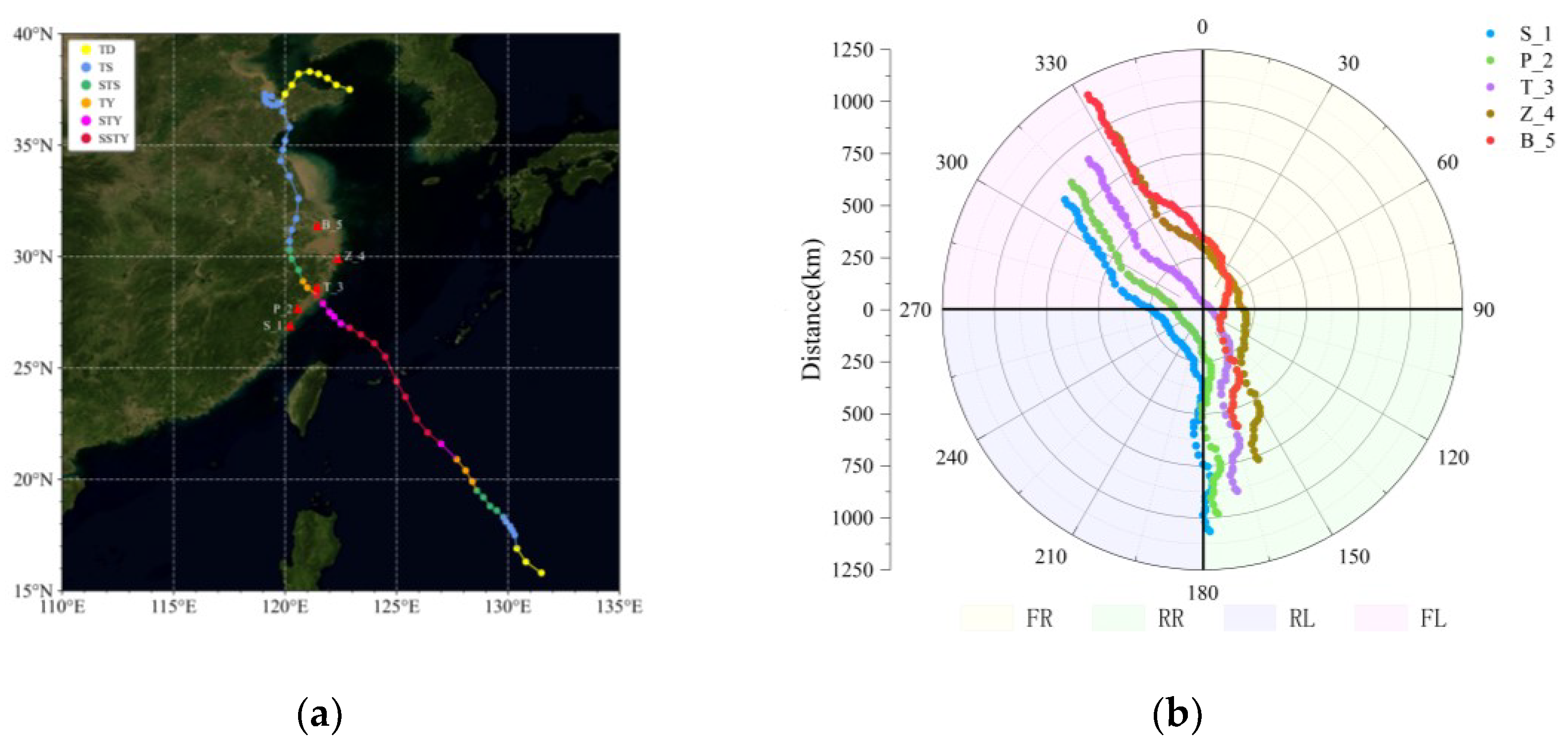
2.1. Super Typhoon Lekima

On 4 August 2019 (China Standard Time: CST = UTC + 8, CST is used throughout), Typhoon Lekima formed in the northwestern tropical Pacific Ocean, the ninth named storm of the 2019 Pacific typhoon season. Lekima then moved steadily in a northwesterly direction with increasing intensity. On 7 August, it developed rapidly from a strong tropical storm to a super typhoon, and remained a super typhoon for 51 h before landfall. At 01:45 on 10 August, it made landfall in Wenling City, Zhejiang Province, China. The minimum sea level pressure was 930 hPa and the maximum wind speed was 52 m s⁻¹. Thereafter, it continued to move north-northwestward through Zhejiang and Jiangsu provinces, then into the western waters of the Yellow Sea. At 20:50 on 11 August, Lekima made its second landfall in Qingdao, Shandong Province (as a tropical storm), and then moved across the Shandong Peninsula and the Bohai Sea. The best-track positions and intensities of Lekima from the China Meteorological Administration’s best-track database [33] are shown in Figure 1a. The locations of the joint observations made during the passage of Typhoon Lekima are indicated by the red triangles in Figure 1a. Typhoon Lekima was characterized by high intensity, severe precipitation, extended duration over land, and serious disaster damage: (1) sea level pressure was low when it made landfall, and it was the third largest typhoon in Zhejiang Province’s history; (2) the impact of Lekima was extremely significant, ranking second in terms of combined disaster-causing intensity among the landfalling typhoons in Zhejiang Province. The heavy rainfall caused by the typhoon’s landfall and transit caused rainfall records to be broken at a total of 19 stations in Zhejiang and Jiangsu provinces. The measured wind speed was the second strongest (61.4 m s⁻¹) of the typhoons that made landfall in Zhejiang Province. (3) After landfall, the typhoon weakened slowly and moved slowly. It remained in Zhejiang Province for 20 h and was the longest-duration super typhoon in Zhejiang Province.

2.2. Joint Observations

Five DWLs were used in the joint observational experiment of this study, distributed from south to north in Sansha Town, Xiapu County, Fujian Province (S_1); Pingyang County, Wenzhou City, Zhejiang Province (P_2); Taizhou City, Zhejiang Province (T_3); Zhoushan City, Zhejiang Province (Z_4); and Baoshan District, Shanghai City (B_5), as indicated by the red triangles in Figure 1a. The DWL types and specific locations corresponding to each station are listed in

Table 1. Details of DWL type and location of the observation sites.

DWL	Location	Type	Longitude (°)	Latitude (°)	Altitude (m)
S_1	SanSha	WindPrint S4000	120.229	26.919	40
P_2	PingYang	Windcube V2	120.573	27.669	254
T_3	TaiZhou	Windcube V2	121.417	28.618	2
Z_4	ZhouShan	Windcube V2	122.367	29.902	10
B_5	BaoShan	WindPrint S4000	121.444	31.391	9

. The analysis period was from 00:00 on 8 August 2019 to 24:00 on 11 August 2019, and the azimuth and relative distance distribution of each DWL relative to the typhoon center are shown in Figure 1b. Here, the center point is the typhoon center, the positive x-axis represents the direction relative to the right side of the typhoon movement, and the positive y-axis represents the direction relative to the front side of the typhoon motion, and each DWL is classified into four quadrants relative to the typhoon direction of motion at any time: rear left (RL), front left (FL), front right (FR), and rear right (RR).

The DWL at locations S_1 and B_5 is a WindPrint S4000, and at P_2, T_3, and Z_4 a Windcube V2. During the observation period, the closest distances of the five DWLs to the typhoon center were 183, 102, 32, 176, and 92 km, in the order in the table. S_1 is located at the East China Field Observation Base in Sansha Town, Xiapu County, Fujian Province, and the meteorological tower (at 120.2317° E, 26.9231° N) is located at a distance of ~400 m from this DWL. S_1 is located on the south side of the meteorological tower, which is <50 m from the coastline, and the base of the meteorological tower is ~10 m higher than the base of S_1.

The WindPrint S4000 was manufactured by Qingdao Hua Hang Environmental Technology Co., Ltd. in China, and the Windcube V2 is a commercial wind measurement lidar developed by Leosphere in France. Both use the DBS (Doppler Beam Swinging) scanning method for wind field detection, with high temporal resolution, and can continuously obtain horizontal wind speed (U), vertical wind velocity (w), wind direction, and signal-to-noise ratio (SNR, i.e., signal effective power/noise effective power (Ps/Pn)), as well as various atmospheric parameters including ground temperature and pressure. The meteorological tower at the Sansha site was equipped with WindMaster Pro three-dimensional ultrasonic anemometers from Gill, UK, at heights of 10, 30, 50, and 70 m. The quality control methods and data preprocessing for the application of WindMaster Pro three-dimensional ultrasonic anemometers in typhoon conditions are detailed in [34,35]; these anemometers are highly reliable in such conditions. Images of the instruments used for the joint observations are shown in Figure 2 (i.e., WindPrint S4000, Windcube V2, and WindMaster Pro), and the main performance parameters are listed in

Table 2. Main performance parameters of the different instruments.

Instruments	Detection Range	Data Update	Wind Speed Range	Wind Speed Accuracy
WindPrint S4000	77.9–2450 m	0.25 Hz	0–75 m s−1	0.1 m s−1
Windcube V2	40–290 m	1 Hz	0–80 m s−1	0.1 m s−1
WindMaster Pro	10–70 m	20 Hz	0–65 m s−1	0.1 m s−1

.

2.3. Data Processing

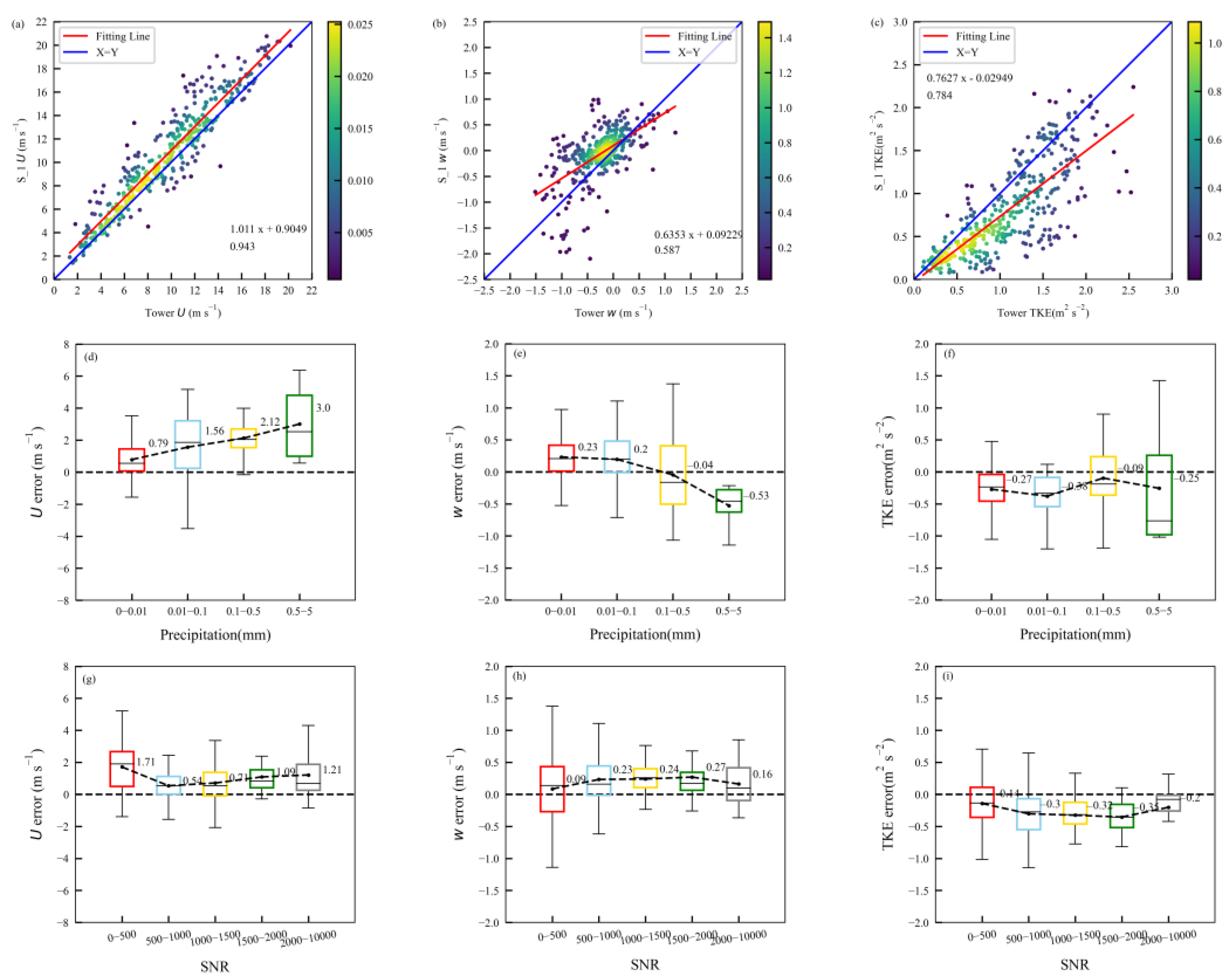
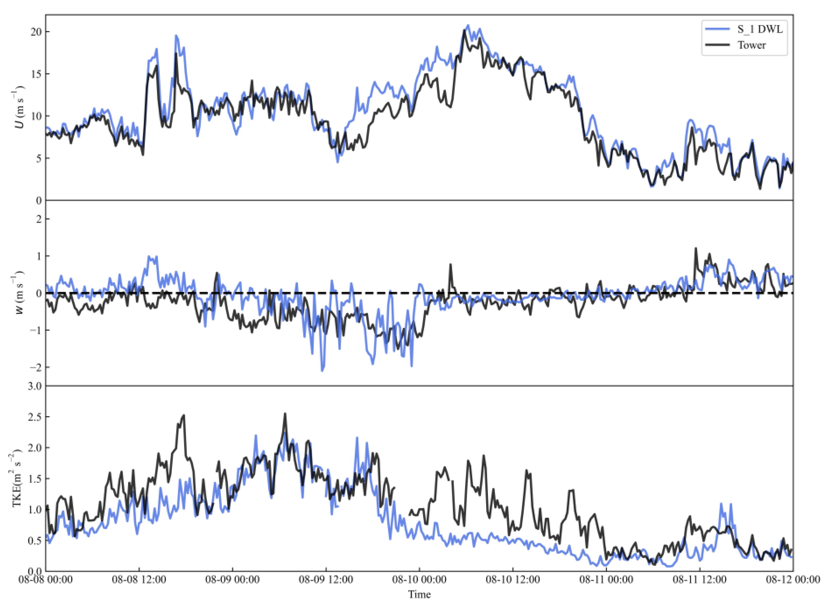
2.3.1. Data Reliability Analysis

DWL observations are affected by the SNR. According to the equipment description, the WindPrint DWL cannot obtain reliable data when the SNR is lower than 7. Therefore, in the process of data quality control, WindPrint DWL data with SNR lower than 7 are directly eliminated, and then the U and w are quality controlled. Random noise and error mean that the wind speed values at individual heights will have large errors, so anomalous values of U and w are eliminated. The U greater than 70 m s⁻¹ are regarded as anomalous values. The w is defined as positive upward and negative downward. When precipitation occurs, the w represents the sum of the vertical movement of air and the sinking movement of precipitation particles. Taking 10 m s⁻¹ as the threshold value of w, w data are discarded when |w| > 10 m s⁻¹. After completing the data quality control, 15 min averages of the U and w were used for analysis.

Since different types of DWL are used in the study, it is necessary to illustrate the reliability of the observations. The Sansha station tower data were used as the standard values, and the data from S_1 were compared with those of the tower. Tower data at 70 m height were compared with S_1 data at 77.9 m to verify the reliability and accuracy of S_1 observational data. Time series of 15 min mean U, w, and TKE were plotted (Figure 3). The U measured by S_1 was generally in good agreement with that measured by the tower. Both increased gradually in the 12 h before typhoon landfall and reached a peak at around 6:00 on 10 August, with a maximum U of ~21 m s⁻¹. After that, the U gradually decreased. The S_1 data were significantly larger than those of the tower in the 12 h before typhoon landfall, probably because the observation height of S_1 was higher than that of the tower. The analysis of the w shows that the trend of w is more consistent, and both have an obvious sinking motion in the 24 h before typhoon landfall. The difference is that the w of S_1 fluctuates dramatically in the 12 h before typhoon landfall, and the w from the tower fluctuates slightly. The TKE from the tower is significantly larger than that of S_1, especially in the 24 h after typhoon landfall. The different time sample resolutions contribute to the differences between the two soundings; the tower data were acquired with fast-response instruments (20 Hz) that capture energetic turbulent processes that cannot be resolved by the DWL.

To further evaluate the accuracy of the WindPrint S4000 in typhoon conditions, the U, w, and TKE from S_1 were linearly fitted to tower observations at the same height (Figure 4a–c) and the errors plotted as functions of precipitation (Figure 4d–f) and SNR (Figure 4g–i). The best fit is obtained for U: the slope of the fitted line is close to 1, with a correlation coefficient of 0.943. The systematic overestimation of S_1 relative to the tower is about 0.9 m s⁻¹. One explanation for this overestimation is natural variability in U itself. Another reason is that measurements are made at a greater height with S_1 than with the tower. Comparing the w, we found that the fit between S_1 and the tower was poor, with a correlation coefficient of 0.587. The WindPrint lidar data points were mainly distributed above the x = y line, indicating that most of the w of S_1 were greater than those of the tower. The w from S_1 was significantly too low (more negative) when the wind speed of the tower was about −1 m s⁻¹, indicating that the sinking motion measured by S_1 was more intense when there was strong sinking motion. Under precipitation conditions, the vertical velocity spectrum introduced by precipitation will affect the identification of the wind spectrum by DWL. The poor fit of w is probably because the precipitation intensified the sinking motion and S_1 could not distinguish the speed of raindrop landing from the w. The TKE value of S_1 is generally smaller than that from the tower: the slope of the fitted line is 0.763, and the correlation coefficient is 0.784. S_1 underestimates TKE at larger values.

DWL uses the Doppler frequency shift of atmospheric aerosols on laser scattered echoes to indirectly obtain parameters of the atmospheric wind field. Previous studies indicated that precipitation has an effect on the accuracy and range of DWL measurements. Combined with the relationship between error and precipitation, the U error of S_1 is mostly positive and increases with increasing precipitation. The w error changes from positive to negative with the increase in precipitation. When the precipitation is 0.5–5 mm, the w error is always negative and its average value reaches −0.53 m s⁻¹. This may be because the w measured by S_1 superimposes the falling speed of raindrops in the case of greater precipitation, which leads to a more negative w than the actual value. The U error does not change significantly with the SNR but is largest for SNR in the range of 0–500. The mean value of the w error is largest when the SNR is 1500–2000, and the maximum of the mean error is 0.27 m s⁻¹, which indicates that there is no obvious relationship between the U or w error and the SNR. The TKE error is not affected by precipitation or SNR (Figure 4f,i).

The results above are for the accuracy of data measured by WindPrint S4000. For Windcube V2, a comparison with radiosonde data during typhoons [36] showed that precipitation affects the missing data rate of Windcube V2 data mainly by affecting the SNR. Also, at heights below 100 m, the data validity of Windcube V2 is not affected by precipitation and precipitation intensity has little effect on the deviation of U measured by Windcube V2.

2.3.2. Data Processing

Turbulent kinetic energy, TKE, may be written as:

$$\mathrm{TKE}= \frac{1}{2}\sqrt{\left(\overline{{u^{\prime }}^2}+\overline{{v^{\prime }}^2}+\overline{{w^{\prime }}^2}\right)},$$

(1)

where $\overline{u^{\prime }{}^2},\overline{v^{\prime }{}^2}, \mathrm{and} \overline{w^{\prime }{}^2}$ are the 15-min averaged perturbation wind components in the x, y, and z directions, respectively; the perturbation velocities $u^{\prime }=u-\overline{u}$; $\overline{u}$ is the mean value over 15 min. $v^{\prime }$ and $w^{\prime }$ are calculated in the same method as $u^{\prime }$.

Helicity is defined as the volume integral of the dot product of velocity and vorticity:

$$H_T=\iiint \overrightarrow{V}\left(\nabla \times \overrightarrow{V}\right)d\tau .$$

(2)

It reflects the strength of the rotation and the movement along the rotation axis. In this paper we use local vertical helicity:

$$H_z=\left(\frac{\partial v}{\partial x}-\frac{\partial u}{\partial y}\right)·w=w\xi ,$$

(3)

where u and v are the horizontal and vertical components of U, respectively, w is vertical wind velocity, and ξ is vertical vorticity. The vertical helicity is the product of vertical velocity and vertical vorticity, which describes the development of vertical upward motion and vertical vorticity, and reflects the characteristics of atmospheric rotation and upward motion in the vertical.

In this study, the wind field observations from S_1 and B_5 were used to calculate the BLH of Typhoon Lekima from 8 August to 11 August, using the same methods as Zhang et al. [16] and Nuo Chen et al. [24]. Five forms of the BLH are calculated: the inflow layer depth (h_infl); the maximum tangential wind speed height (h_umax); and typhoon BLH based on helicity (h_H), TKE (h_TKE), and SNR (h_SNR).

$$h_{\mathit{infl}}=H\left({10\%V}_{\mathit{max}}\right),$$

(4)

$$h_{\mathit{umax}}=H\left(U_{\mathit{max}}\right),$$

(5)

$$h_H=H\left(\mathit{max}\left(\left|\frac{\partial H_{\mathrm{zi}}}{\partial z_i}\right|\right)\right),$$

(6)

$$h_{\mathit{SNR}}=H\left(\mathit{max}\left(\left|\frac{\partial {\mathrm{SNR}}_i}{\partial z_i}\right|\right)\right),$$

(7)

$$h_{\mathit{TKE}}=H\left(\mathit{max}\left(\left|\frac{\partial {\mathrm{TKE}}_i}{\partial z_i}\right|\right)\right),$$

(8)

where V_max is the maximum radial wind speed, and the depth of the inflow layer (h_infl) indicates the height where 10% of V_max is located; $U_{\mathit{max}}$ is the maximum value of the tangential wind, and h_umax is the height where the maximum tangential wind speed is located; H_Z is the vertical helicity; Z_i is the height at a vertical level; SNR is signal to noise ratio; and TKE refers to the turbulent kinetic energy. h_H represents the height corresponding to the maximum value of the absolute value of the first-order vertical derivative of the helicity with height; h_SNR and h_TKE are calculated by the same method as h_H.

The typhoon path is obtained from best track data from the Shanghai Typhoon Research Institute of the China Meteorological Administration, and the location of the typhoon center is obtained by linear interpolation of the latitude and longitude from the best track. In calculating the tangential and radial winds for each DWL, the typhoon’s moving speed and direction are also obtained from the latitude and longitude between two points based on the best track data, and the typhoon’s moving speed is subtracted from the actual tangential and radial winds obtained from the DWL data to obtain the tangential and radial winds relative to the typhoon’s motion. In this study, both the tangential and radial winds are used relative to the direction of motion of the typhoon.

3. Result

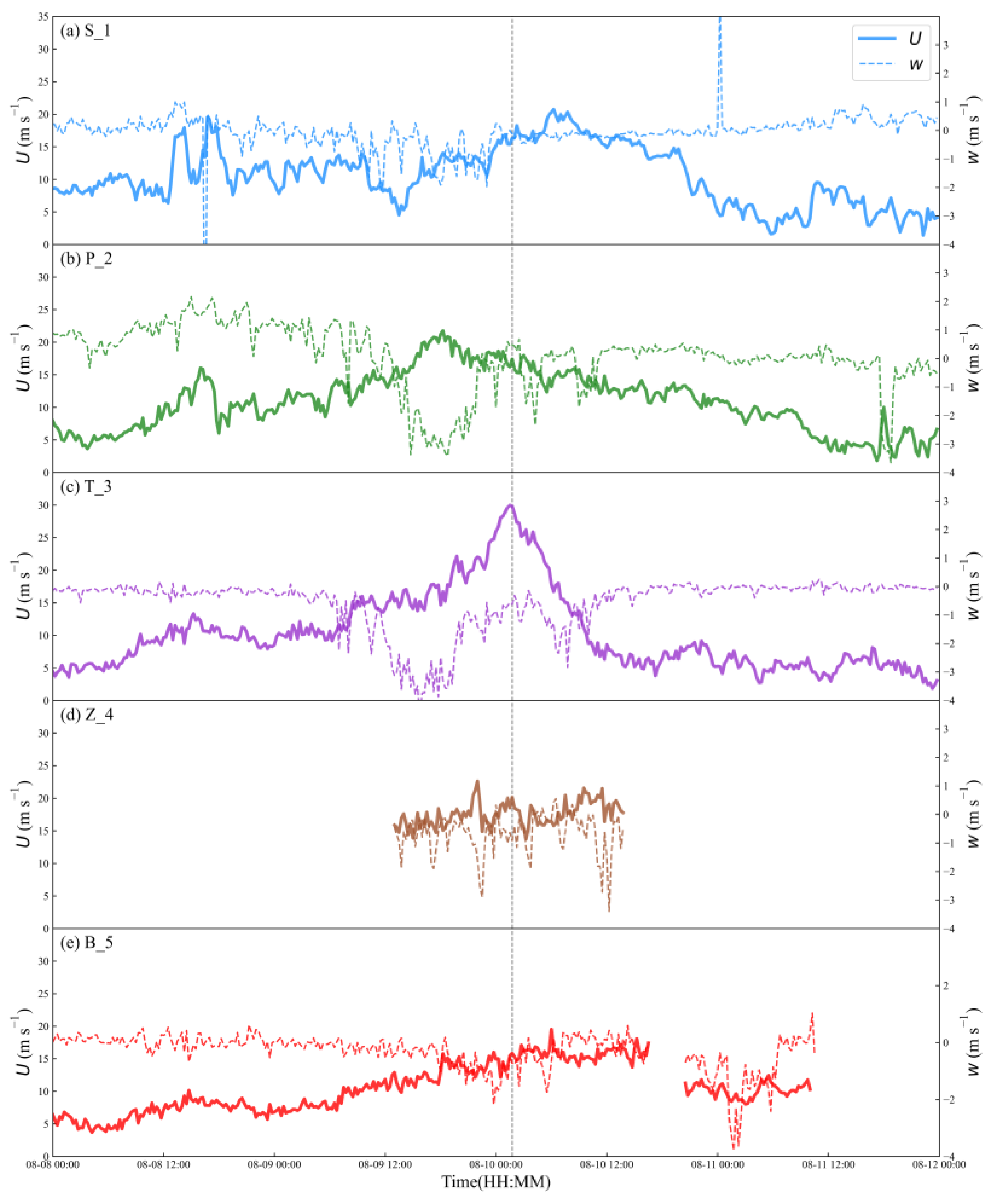
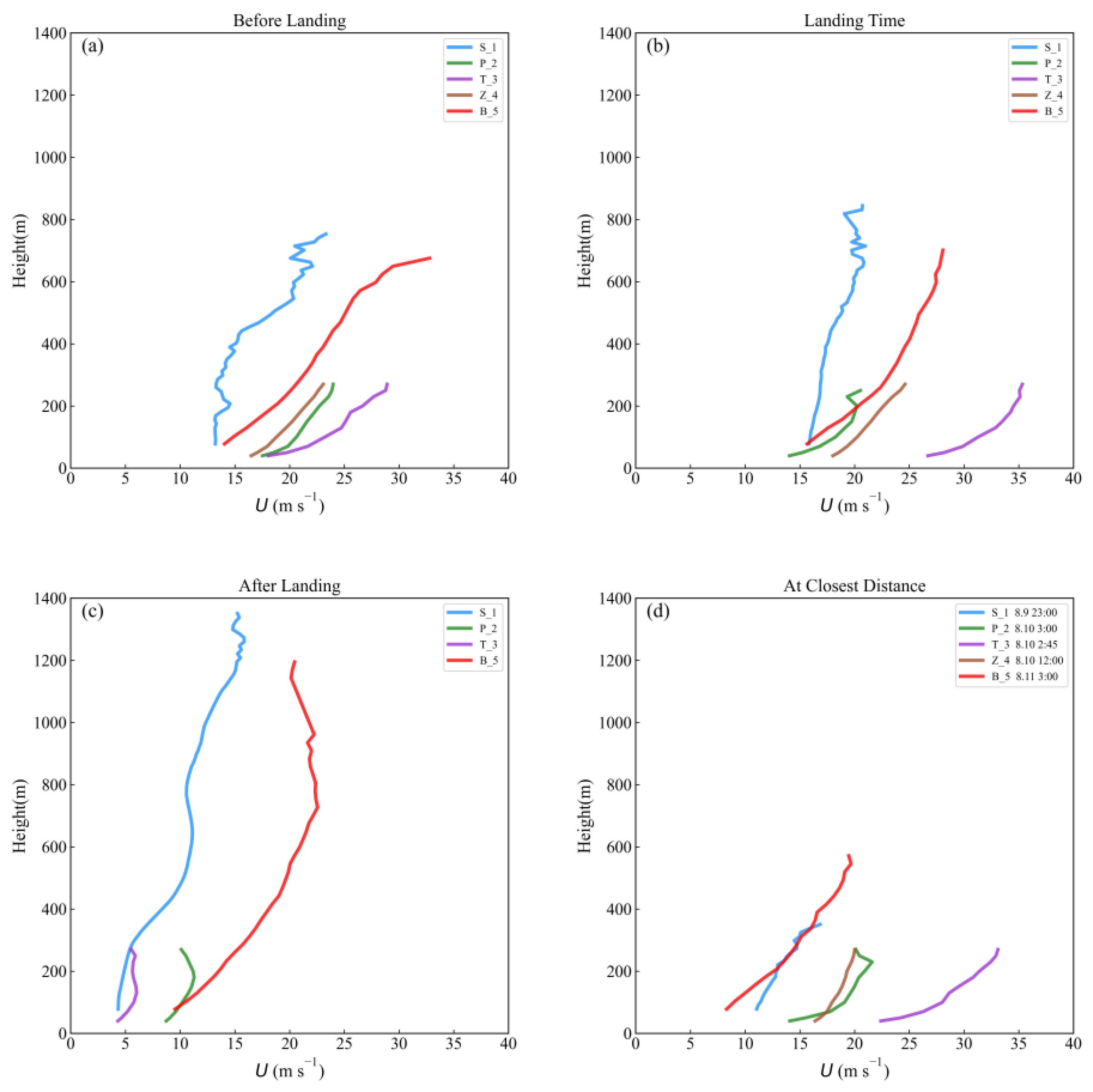
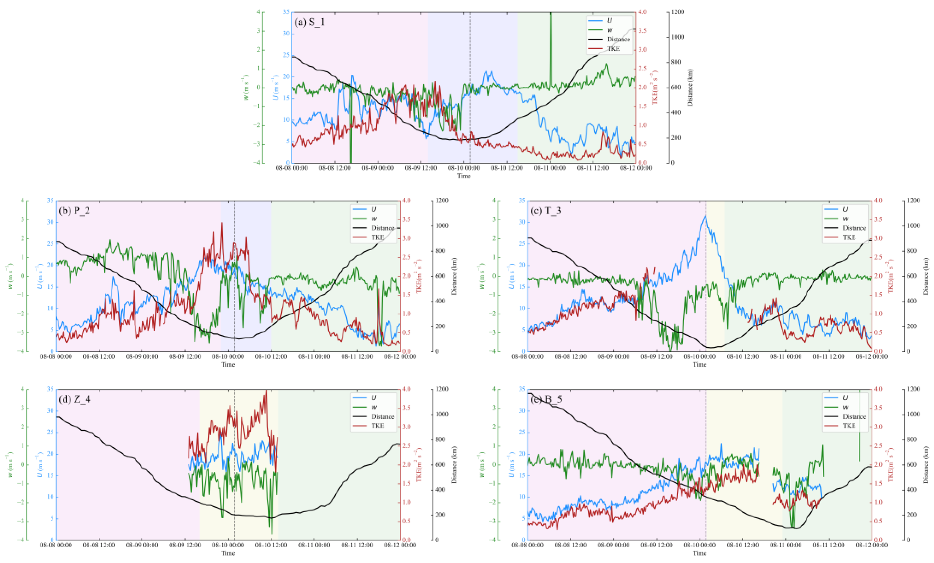
3.1. Boundary Layer Wind Field Characteristics

The observations of each DWL at the same height (WindPrint and Windcube at 77.9 m and 70 m, respectively) from 8 August to 11 August were selected. Fifteen minute samples were used for analysis, and the U and w were averaged arithmetically to plot their changes over time (Figure 5). The U and w are indicated by solid and dashed lines of different colors, respectively. The w greater than zero indicates an updraft, and the black dashed line is the time of typhoon landfall.

S_1 (Figure 5a) showed a decrease and then increase in U from 6:00 to 18:00 on 9 August, and the U decreased to its lowest at around 12:00 on 9 August. This is because the typhoon intensity decreased from super to strong typhoon at this time. After that, the U gradually increased and reached its maximum at 6:00 on 10 August (about 20 m s⁻¹). Overall, the average U before typhoon landfall (11.06 m s⁻¹) was greater than that after landfall (9.89 m s⁻¹). Significant downdraft was observed before typhoon landfall, and the maximum downdraft was about −2.2 m s⁻¹. The w was close to zero after typhoon landfall, and the w varied between −2.2 and 0.9 m s⁻¹ over the whole study period.

At P_2, the U (Figure 5b) showed a trend of first increasing and then gradually decreasing, reaching the maximum of ~22 m s⁻¹ at 18:00 on 9 August. The average U before landfall (11.94 m s⁻¹) was greater than that after landfall (9.76 m s⁻¹). Before 13:00 on 9 August, P_2 updrafts dominated, suddenly switching to violent downdraft, with the maximum downdraft reaching −3.4 m s⁻¹. During the study period, the w varied between −3.66 and 2.16 m s⁻¹.

At T_3, the trend of the U (Figure 5c) was increasing first and then decreasing, and the U reached the maximum of 30 m s⁻¹ at the time of typhoon landfall. The average U before typhoon landfall (12.28 m s⁻¹) was larger than that after landfall (8.05 m s⁻¹). Downdraft was observed at T_3 during most of the study period, with an average w of −0.58 m s⁻¹. From 7:00 on 9 August, there was a significant downdraft, with the w reaching the maximum (−4 m s⁻¹) at about 18:00 on 9 August. There was still an obvious downdraft after typhoon landfall.

At Z_4, the average U (Figure 5d) during the observation period (13:00 on 9 August to 13:45 on 10 August) was 17 m s⁻¹ and the average w was −0.68 m s⁻¹. There was a strong downdraft before and after typhoon landfall, with the w ranging from −3.40 to 0.55 m s⁻¹.

At B_5, the U (Figure 5e) also increased first and then decreased, but was small overall. The average U was 10.43 m s⁻¹, and the U reached its maximum (20 m s⁻¹) at 6:00 on 10 August. Similarly, before typhoon landfall, there was a downdraft. At about 2:00 on 11 August, there was a strong downdraft (−3.7 m s⁻¹) at B_5, which may have been caused by precipitation.

The variations of U with height for DWLs at 8 h before typhoon landfall, at the moment of landfall, 8 h after landfall, and at the closest distance to the typhoon center are plotted respectively (Figure 6). It can be seen that 8 h before typhoon landfall (Figure 6a), the closer each DWL is to the typhoon center, the greater the wind speed, except for S_1, which is located in the left rear quadrant of the typhoon. At the moment of typhoon landfall (Figure 6b), compared with the wind profile before typhoon landfall, there is little difference in the valid data height of WindPrint S4000. The valid data height of B_5 and S_1 is about 700 m. In addition, the U of DWLs increases, except for P_2, which slightly decreases. At 8 h after typhoon landfall (Figure 6c), the U of each DWL decreases and is smaller than that before typhoon landfall, and the valid data height of WindPrint S4000 DWL reaches higher, 1195 m and 1351 m for B_5 and S_1, respectively. In summary, the valid data height of WindPrint S4000 DWL was affected by the typhoon; the valid data height after the typhoon landfall was greater than the typhoon landfall moment and before the typhoon landfall. The valid data height of Windcube V2 was maintained at 270 m.

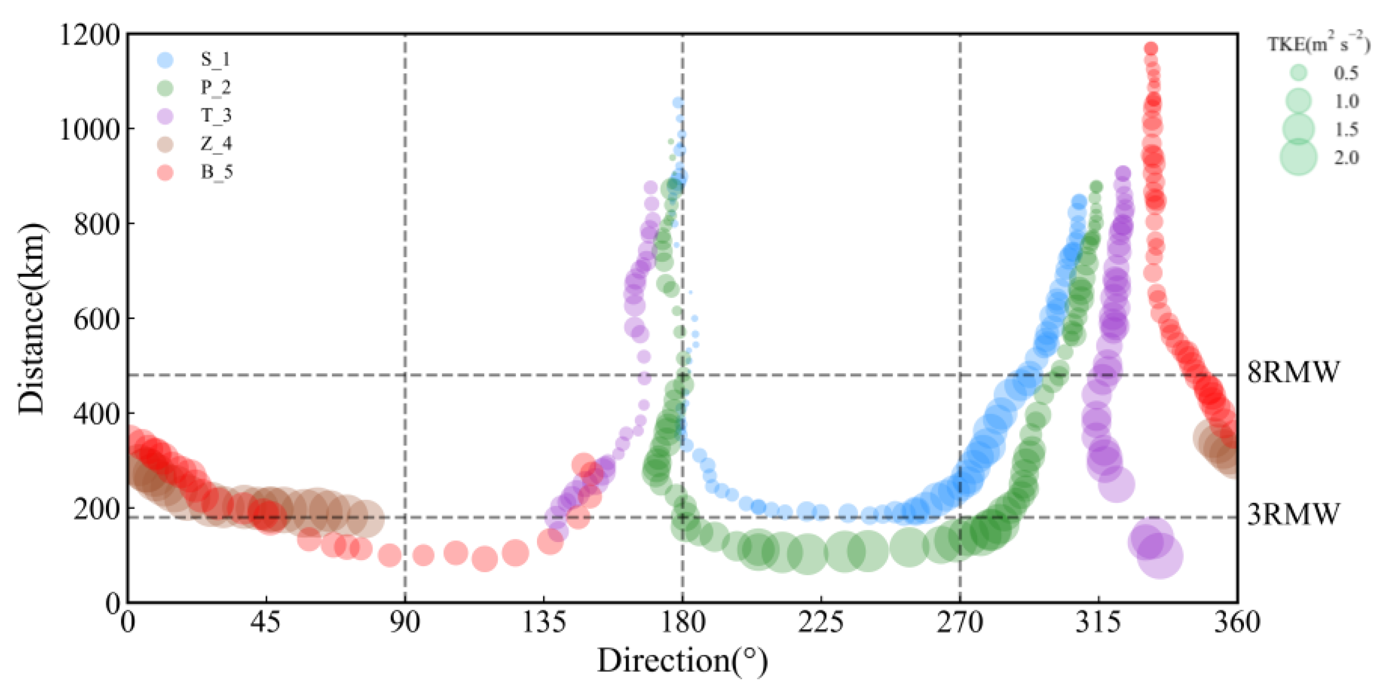
3.2. Turbulent Kinetic Energy

Figure 7 displays the time variation of the mean values at altitudes of 70–200 m of U (blue), w (green), TKE (red), and distance to typhoon center (black) for the five DWLs. A correlation analysis shows that the TKE of P_2, T_3, Z_4, and B_5 has the same trend as U, whereas the TKE of S_1 is inconsistent with the trend of U. The TKE of S_1 (Figure 7a) is larger from 1:00 to 18:00 on 9 August, with a mean of 1.66 m² s⁻², and reaches the maximum (2.17 m² s⁻²) at 16:00 on 9 August. Meanwhile, the U decreases and then increases, and there is a strong downdraft with large vertical fluctuations, thus leading to a large TKE. The TKE of S_1 is significantly larger before typhoon landfall than after typhoon landfall, with mean values of 1.11 m² s⁻² and 0.34 m² s⁻², respectively. P_2 has a large TKE (>2 m² s⁻²) from 16:00 on 9 August to 6:00 on 10 August and reaches a maximum value (3.42 m² s⁻²) at 22:15 on 9 August. At about 13:00 on 9 August, the w changes from positive to negative, and a strong downdraft appears, at which time the TKE increases rapidly. T_3 has missing data from 12:00 on 9 August to 12:00 on 10 August, but in the part where data are available the TKE follows the same trend as the U. Z_4 is observed as a mobile observation, over the period 13:00 on 9 August to 13:00 on 10 August, when its TKE is larger than other observations (the mean value is 2.86 m² s⁻²) and reaches a maximum value of 3.99 m² s⁻² at 10:45 on 10 August. The TKE of B_5 reaches a maximum of 2.00 m² s⁻² at 12:15 on 10 August.

In order to study the changes of TKE of each DWL at different orientations and distances from the typhoon center, the TKE of each DWL was plotted against orientation and distance (Figure 8) and the mean TKEs of each DWL located at different stages of the typhoon center before and after landfall were calculated (

Table 3. Mean TKE (m² s⁻²) of each DWL located at different stages of the typhoon center before and after landfall.

Observations	Before Landfall >8RMW	Before Landfall 3–8RMW	Before Landfall <3RMW	After Landfall <3RMW	After Landfall 3–8RMW	After Landfall >8RMW
S_1	0.809	1.426	/	/	0.403	0.269
P_2	0.688	1.143	2.506	2.008	1.057	0.455
T_3	0.999	1.622	2.696	/	0.725	0.613
Z_4	/	2.753	/	/	3.003	/
B_5	0.701	1.292	/	1.111	1.605 0.994	/

). S_1 and P_2 were always to the left of the typhoon center, while T_3, Z_4, and B_5 were located to the right of the typhoon center. The observation period of Z_4 is limited (from 13:00 on 9 August to 13:00 on 10 August), and the distance of Z_4 from the typhoon center is always 3–8 times the radius of maximum wind (RMW); outer RMW is 60 km [37]. Overall, the closer the DWL is to the typhoon center before and after landfall, the larger the mean TKE.

Before typhoon landfall, when S_1, P_2, T_3, and B_5 were >8 RMW from the center of the typhoon, their mean TKE values were 0.809, 0.688, 0.999, and 0.701 m² s⁻², respectively. As the typhoon approached, when the distance from the typhoon center was 3–8 RMW, the increases of mean TKE were similar, with values of 0.617, 0.455, 0.623, and 0.591 m² s⁻², respectively. In the inner core of the typhoon (<3RMW), the increase of mean TKE at P_2 and T_3 was even greater, with the mean TKE values increasing by 1.363 m² s⁻² and 1.074 m² s⁻², respectively. After the typhoon made landfall and was moving gradually northward, the mean TKE of B_5 and T_3 located to the right of the typhoon center changed little, while the TKE of S_1 and P_2 located to the left of the typhoon center decreased rapidly. Comparing the changes of TKE before and after landfall of each DWL, the TKE values of S_1, P_2, and T_3 before typhoon landfall were larger than after landfall, and the TKE of Z_4 and B_5 were larger after than before landfall; however, the difference was not large, which might be caused by the closer distance between the two DWLs and the typhoon center after landfall.

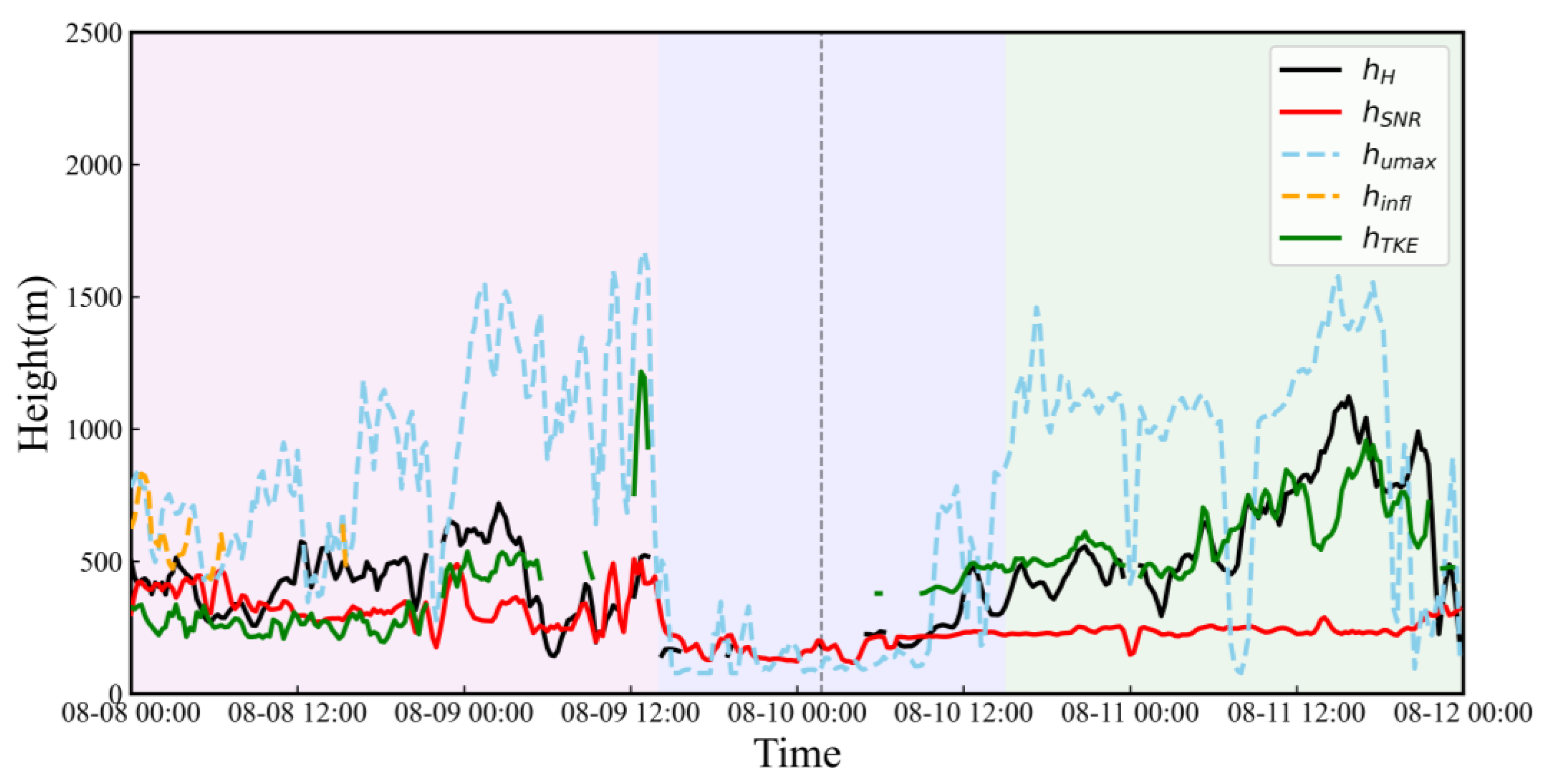
3.3. Boundary Layer Height

Figure 9 shows the variation with time of the five different forms of the BLH of S_1 calculated using Equations (4)–(8). The BLH calculated by the various methods reaches its lowest value in the 10 h before and after the typhoon landfall, and each BLH gradually increases as the typhoon moves away after the landfall. The mean values of the BLHs of different methods were calculated separately for the DWLs located in different quadrants relative to the typhoon center (

Table 4. Mean values of BLHs when S_1 is in different quadrants of the typhoon center.

Boundary Layer Height (m)	FL	RL	RR
hH (m)	426	253	623
hTKE (m)	352	433	613
hSNR (m)	333	187	242
humax (m)	898	233	975
hinfl (m)	629	/	/

). In FL, h_H, h_TKE, and h_SNR have the same trend and similar values, with mean values of 426, 352, and 333 m, respectively. Missing data affected h_H and h_TKE more in the RL, and the data are not representative, but h_SNR has a mean value of 187 m. In RR, h_H and h_TKE gradually increased as the typhoon moved away, with mean values of 623 and 613 m, respectively. The value of h_SNR hardly changed after typhoon landfall, with a mean value of 242 m. h_infl and h_umax have similar values, but h_infl is missing more data and will not be discussed in the subsequent analysis. h_umax is larger than other heights, and during FL, h_umax gradually increased, with a mean value of 898m; in RL, h_umax decreased sharply with a mean value of 233 m. After typhoon landfall, h_umax increased gradually as the typhoon center moved away, with a mean value of 975 m in RR.

Figure 10 shows the changes of various BLHs from B_5 with time. The data quality at B_5 is poor. h_umax is larger than other heights and gradually decreased as the typhoon center approached B_5, with a mean value of 550 m before typhoon landfall (

Table 5. Mean values of BLHs when B_5 is in different quadrants of the typhoon center.

Boundary Layer Height (m)	FR	RR	FL
hH (m)	303	134	250
hTKE (m)	/	/	287
hSNR (m)	171	154	347
humax (m)	463	417	550
hinfl (m)	/	223	/

), and was almost constant after landfall, with a mean value of 440 m. h_SNR had a mean value of 347 m before typhoon landfall and tended to stabilize after landfall, with a mean value of 163 m. The mean value of h_SNR before typhoon landfall was 347 m, and after landfall tended to be stable, with a mean value of 163 m. The well-defined values of h_H and h_TKE are concentrated between 3:40 and 22:00 on 8 August, when h_H and h_TKE were similar, with the same trend and mean values of 320 and 295 m, respectively.

In summary, the TBLH gradually decreased before typhoon landfall and gradually increased after landfall. The trend of the TBLH calculated by helicity and TKE is consistent, and both can determine the TBLH well, while h_umax is larger than the height calculated by other methods.

4. Discussion

4.1. Reliability Discussion

Under precipitation conditions, the vertical velocity spectrum introduced by precipitation will affect the identification of the wind spectrum by DWL. Therefore, DWL has an impact on the measurement of w under precipitation conditions. Meanwhile, we selected a longer period of time (13 August–31 October 2020) to screen the w measured by DWL during the precipitation period, and obtained 4186 samples to study the relationship between w error and precipitation intensity (Figure 11). We found that the w error was mainly concentrated between ±1 m s⁻¹, when the precipitation intensity was less than 1 mm/h, and only when the precipitation intensity was greater than 1 mm/h, the w produced a large negative error. The number of samples with negative error greater than 2 m s⁻¹ is: 277, accounting for 6.6% of all samples, and we think such an error range is acceptable.

4.2. TKE Discussion

Data from stations at the same time and at the same distance from the typhoon center but in different quadrants were selected for analysis (

Table 6. TKE values for each station at the same time, at the same distance from the typhoon center, but distributed in different quadrants. Color shading indicates the quadrant, as in Figure 1b.

Time	TKE of S_1 (m2 s−2)	TKE of P_2 (m2 s−2)	TKE of T_3 (m2 s−2)	TKE of Z_4 (m2 s−2)	TKE of B_5 (m2 s−2)	Distance (km)
8.10 5:00	0.45			2.7		200
8.10 10:00	0.51				1.9	250
8.10 12:00		1.13		2.92		180
8.10 13:00		0.95			1.55	200
8.10 13:00				2.48	1.55	200
8.10 15:00			0.87		1.6	190

). At 5:00, 10:00, and 12:00 on 10 August, S_1 and P_2 were located in the RL quadrant of the typhoon while Z_4 and B_5 were located in the FR quadrant. The TKE values in the FR quadrant of the typhoon were significantly larger (2.50–6.00 times higher) than those in the RL quadrant. At 13:00 and 15:00 on 10 August, P_2 and T_3 were located in the RR quadrant of the typhoon and B_5 was located in the FR quadrant. The TKE value in the FR quadrant of the typhoon was about 1.7 times higher than that in the RR quadrant. At 13:00 on 10 August, both Z_4 and B_5 were located in the FR quadrant of the typhoon, but the TKE of B_5 was smaller because B_5 was located in the urban area and Z_4 was located in the island. The wind speed in the urban area was strongly modified by the surface friction, resulting in a smaller TKE value.

To sum up, the magnitude of TKE is related not only to the U, but also to the presence of a strong downdraft that leads to a rapid increase of TKE. The magnitudes of TKE in different quadrants of Typhoon Lekima were different, with the TKE in the FR quadrant being larger than that in the RL and RR quadrants. Due to the influence of surface friction, the TKE on the island was larger than the TKE in the urban area.

4.3. BLH Discussion

Five methods were used in the paper to calculate the TBLH of S_1 and B_5. Among them, h_infl and h_umax are the most common methods to calculate the TBLH; in our calculation, the results of h_infl and h_umax are similar, but h_infl has a lot of missing data. The SNR-based method is a common method in conventional atmospheric environments, and this method has almost no significant changes after typhoon landfall, which is inconsistent with the traditional TBLH understanding [16,24]. The variation in TBLH calculated for h_H, h_TKE, and h_umax is consistent with the classical understanding, which gradually decreased before typhoon landfall and gradually increased after landfall. The h_H and h_TKE have similar values, while h_umax is larger than the height calculated by other methods.

5. Conclusions

Turbulence processes in the TBL play an important role in the maintenance and intensification of typhoons. In particular, the finescale structure in the lower boundary layer is very important for the prediction of typhoon intensity. The detection of finescale structures in the TBL has long been difficult due to instrumental limitations. In the critical range of 50–500 m, there is still a lack of observational data of the finescale structure, and the finescale structure of the TBL and its turbulence characteristics require further study. As a new type of remote sensing technique, DWL is widely used in wind field detection, but has been applied less to TBL circulation. Based on previous research, we used multiple ground-based DWLs to detect the TBL of a typical typhoon. The main purpose of our diagnostic study of finescale structures was to evaluate the ability of DWL to detect finescale structures in the TBL. The conclusions are as follows:

(1) DWL provides a new side for the study of turbulence structure under typhoon conditions, which can effectively complement and extend the high-precision observations on the surface. We believe that DWL combined with tower observations can provide more insights for the study of boundary layer turbulence in the future.

(2) Further research shows that the TKE diagnosed based on observational data is generally larger before typhoon landfall than after, and its magnitude is not only related to the change of U, but also has a stronger relationship with fluctuations of w. When the observations are at the same time, at the same distance from the typhoon center, the TKE is strongly related to the quadrant where the observation is located. When the observation is located in the FR quadrant of the typhoon center, the TKE is significantly larger than in the RL and RR. In addition to the quadrant where the observation is located, the TKE is also related to the location of the observation. The observations located on the island are larger than those in the urban area.

(3) The TBLHs of S_1 and B_5 were diagnosed using multiple methods based on the WindPrint S4000 DWL data. The TBLH of S_1 reaches its lowest value in the 10 h before and after typhoon landfall; after typhoon landfall, the TBLH gradually increases as the typhoon moves away, which is consistent with classical understanding. The TBLH of B_5 also decreases before typhoon landfall. The trends of the TBLH of S_1 and B_5 based on helicity and TKE are consistent, and both can determine the TBLH well, while h_umax is larger than the height calculated by other methods.

(4) DWL can be used to detect the TBL structure, at least under the typhoon outer circulation and weak precipitation. The performance of different DWLs may vary, and DWLs with strong signal power have a larger detection range and the data may be relatively more reliable. Thus, a greater number of DWLs and more powerful DWLs need to be utilized for detection and wind measurement in future TBL observation strategies. This study has confirmed the ability of DWL to observe the structure of the typhoon boundary layer, which can be used to detect the characteristics of landfalling typhoons and provide a reference for the evaluation and improvement of models.

Our results are based on only a few DWL experiments in specific areas for a specific case, and the representativeness of the conclusions needs to be verified by more experiments and case studies in the future. However, we believe that DWL, a new remote sensing detection tool, has good prospects of finding a useful application in studying the finescale structure of typhoons and other strong convective weather.

References

1. Smith, R.K.; Montgomery, M.T. Hurricane boundary-layer theory. Q. J. Roy. Meteor. Soc. 2010, 136, 1665–1670. [Google Scholar] [CrossRef] [Green Version]
2. Smith, R.K.; Montgomery, M.T.; Vogl, S. A critique of Emanuel’s hurricane model and potential intensity theory. Q. J. Roy. Meteor. Soc. 2008, 134, 551–561. [Google Scholar] [CrossRef] [Green Version]
3. Rotunno, R.; Chen, Y.; Wang, W.; Davis, C.; Dudhia, J.; Holland, G.J. Large-Eddy Simulation of an Idealized Tropical Cyclone. B. Am. Meteorol. Soc. 2009, 90, 1783–1788. [Google Scholar] [CrossRef]
4. Braun, S.A.; Tao, W.K. Sensitivity of high-resolution simulations of Hurricane Bob (1991) to planetary boundary layer parameterizations. Mon. Weather Rev. 2000, 128, 3941–3961. [Google Scholar] [CrossRef] [Green Version]
5. Smith, R.K.; Thomsen, G.L. Dependence of tropical-cyclone intensification on the boundary-layer representation in a numerical model. Q. J. Roy. Meteor. Soc. 2010, 136, 1671–1685. [Google Scholar] [CrossRef]
6. Zhang, J.A.; Rogers, R.F.; Tallapragada, V. Impact of Parameterized Boundary Layer Structure on Tropical Cyclone Rapid Intensification Forecasts in HWRF. Mon. Weather Rev. 2017, 145, 1413–1426. [Google Scholar] [CrossRef]
7. Troen, I.; Mahrt, L. A simple model of the atmospheric boundary layer: Sensitivity to surface evaporation. Bound-lay Meteorol. 1986, 37, 129–148. [Google Scholar] [CrossRef]
8. Hong, S.Y.; Pan, H.L. Nonlocal boundary layer vertical diffusion in a Medium-Range Forecast Model. Mon. Weather Rev. 1996, 124, 2322–2339. [Google Scholar] [CrossRef] [Green Version]
9. Emanuel, K.A. An air–sea interaction theory for tropical cyclones. Part I: Steady-state maintenance. J. Atmos. Sci. 1986, 43, 585–605. [Google Scholar] [CrossRef]
10. Powell, M.D. Boundary layer structure and dynamics in outer hurricane rainbands. Part II: Downdraft modification and mixed layer recovery. Mon. Weather Rev. 1990, 118, 918–938. [Google Scholar] [CrossRef] [Green Version]
11. Anthes, R.A.; Chang, S.W. Response of the hurricane boundary layer to changes of sea surface temperature in a numerical model. J. Atmos. Sci. 1978, 35, 1240–1255. [Google Scholar] [CrossRef] [Green Version]
12. Rotunno, R.; Bryan, G.H. The Maximum Intensity of Tropical Cyclones in Axisymmetric Numerical Model Simulations. Mon. Weather Rev. 2009, 137, 1770–1789. [Google Scholar] [CrossRef]
13. Smith, R.K.; Montgomery, M.T.; Van Sang, N. Tropical cyclone spin-up revisited. Q. J. Roy. Meteor. Soc. 2009, 135, 1321–1335. [Google Scholar] [CrossRef] [Green Version]
14. Hong, S.Y.; Noh, Y.; Dudhia, J. A new vertical diffusion package with an explicit treatment of entrainment processes. Mon. Weather Rev. 2006, 134, 2318–2341. [Google Scholar] [CrossRef] [Green Version]
15. Kepert, J.D. Slab- and height-resolving models of the tropical cyclone boundary layer. Part I: Comparing the simulations. Q. J. Roy. Meteor. Soc. 2010, 136, 1686–1699. [Google Scholar] [CrossRef]
16. Zhang, J.A.; Rogers, R.F.; Nolan, D.S.; Marks, F.D. On the Characteristic Height Scales of the Hurricane Boundary Layer. Mon. Weather Rev. 2011, 139, 2523–2535. [Google Scholar] [CrossRef]
17. Von Engeln, A.; Teixeira, J. A Planetary Boundary Layer Height Climatology Derived from ECMWF Reanalysis Data. J. Climate 2013, 26, 6575–6590. [Google Scholar] [CrossRef]
18. Frisch, U.; Donnelly, R.J. Turbulence: The Legacy of A. N. Kolmogorov. Phys. Today 1996, 49, 82–84. [Google Scholar] [CrossRef] [Green Version]
19. Moffatt, H.; Tsinober, A. Helicity in laminar and turbulent flow. Annu. Rev. Flud. Mech. 1992, 24, 281–312. [Google Scholar] [CrossRef]
20. Bogner, P.B.; Barnes, G.M.; Franklin, J.L. Conditional instability and shear for six hurricanes over the Atlantic Ocean. Weather Forecast. 2000, 15, 192–207. [Google Scholar] [CrossRef]
21. Vollaro, D.; Molinari, J. Extreme Helicity and Intense Convective Towers in Hurricane Bonnie. Mon. Weather Rev. 2008, 136, 4355–4372. [Google Scholar] [CrossRef]
22. Vollaro, D.; Molinari, J. Distribution of Helicity, CAPE, and Shear in Tropical Cyclones. J. Atmos. Sci. 2010, 67, 274–284. [Google Scholar] [CrossRef] [Green Version]
23. Onderlinde, M.J.; Nolan, D.S. Environmental Helicity and Its Effects on Development and Intensification of Tropical Cyclones. J. Atmos. Sci. 2014, 71, 4308–4320. [Google Scholar] [CrossRef] [Green Version]
24. Chen, N.; Tang, J.; Zhang, J.A.; Ma, L.-M.; Yu, H. On the distribution of helicity in the tropical cyclone boundary layer from dropsonde composites. Atmos. Res. 2021, 249, 105298. [Google Scholar] [CrossRef]
25. Ma, L.-M.; Bao, X.-W. Parametrization of Planetary Boundary-Layer Height with Helicity and Verification with Tropical Cyclone Prediction. Bound-Lay Meteorol. 2016, 160, 569–593. [Google Scholar] [CrossRef]
26. Zhang, J.A. Effects of Roll Vortices on Turbulent Fluxes in the Hurricane Boundary Layer. Bound-Lay Meteorol. 2008, 128, 173–189. [Google Scholar] [CrossRef]
27. Morrison, I.; Businger, S.; Marks, F.; Dodge, P.; Businger, J. An Observational Case for the Prevalence of Roll Vortices in the Hurricane Boundary Layer. J. Atmos. Sci. 2005, 62, 4121. [Google Scholar] [CrossRef]
28. Zhu, P. Simulation and parameterization of the turbulent transport in the hurricane boundary layer by large eddies. J. Geophys. Res. 2008, 113. [Google Scholar] [CrossRef]
29. Zhang, J.A.; Nolan, D.S.; Rogers, R.F.; Tallapragada, V. Evaluating the Impact of Improvements in the Boundary Layer Parameterization on Hurricane Intensity and Structure Forecasts in HWRF. Mon. Weather Rev. 2015, 143, 3136–3155. [Google Scholar] [CrossRef]
30. Powell, M.D.; Vickery, P.J.; Reinhold, T.A. Reduced drag coefficient for high wind speeds in tropical cyclones. Nature 2003, 422, 279–283. [Google Scholar] [CrossRef] [PubMed]
31. Bucci, L.R.; O’Handley, C.; Emmitt, G.D.; Zhang, J.A.; Ryan, K.; Atlas, R. Validation of an Airborne Doppler Wind Lidar in Tropical Cyclones. Sensors 2018, 18, 4288. [Google Scholar] [CrossRef] [Green Version]
32. Zhang, J.; Atlas, R.; Emmitt, G.; Bucci, L.; Ryan, K. Airborne Doppler Wind Lidar Observations of the Tropical Cyclone Boundary Layer. Remote Sens. 2018, 10, 825. [Google Scholar] [CrossRef] [Green Version]
33. Feng, J.; Lu, X.; Yu, H.; Zhang, W.; Ying, M.; Fan, Y.; Zhu, Y.; Chen, D. An Overview of the China Meteorological Administration Tropical Cyclone Database. J. Atmos. Ocean. Tech. 2014, 31, 287–301. [Google Scholar] [CrossRef] [Green Version]
34. Tang, J.; Byrne, D.; Zhang, J.A.; Wang, Y.; Lei, X.-T.; Wu, D.; Fang, P.-Z.; Zhao, B.-K. Horizontal Transition of Turbulent Cascade in the Near-Surface Layer of Tropical Cyclones. J. Atmos. Sci. 2015, 72, 4915–4925. [Google Scholar] [CrossRef]
35. Fang, P.; Zhao, B.; Zeng, Z.; Yu, H.; Lei, X.; Tan, J. Effects of Wind Direction on Variations in Friction Velocity With Wind Speed Under Conditions of Strong Onshore Wind. J. Geophys. Res-Atmos. 2018, 123, 7340–7353. [Google Scholar] [CrossRef]
36. Tang, S.M.; Guo, Y.; Wang, X.; Tang, J.; Li, T.T.; Zhao, B.K.; Zhang, S.; Li, Y.P. Validation of Doppler Wind Lidar during Super Typhoon Lekima (2019). Front. Earth Sci. 2020, 15. [Google Scholar] [CrossRef]
37. Dai, H.; Zhao, K.; Li, Q.; Lee, W.C.; Ming, J.; Zhou, A.; Fan, X.; Yang, Z.; Zheng, F.; Duan, Y. Quasi-Periodic Intensification of Convective Asymmetries in the Outer Eyewall of Typhoon Lekima (2019). Geophys. Res. Lett. 2021, 48, e2020GL091633. [Google Scholar] [CrossRef]
Figure 1. (a) Track and intensity of Super Typhoon Lekima and location of observation sites. (TD—Tropical Disturbance and Tropical Depression, TS—Tropical Storm, STS—Severe Tropical Storm, TY—Typhoon, STY—Severe Typhoon, and SSTY—Super Typhoon). (b) The azimuth and relative distance distribution of each DWL relative to the typhoon center. (Front left (FL), Front right (FR), Rear left (RL), Rear right (RR)).
Remotesensing 13 04810 g001
Figure 2. Instruments used for the joint observations. (a) Windprint S4000 DWL, (b) Windcube V2 DWL, and (c) WindMaster Pro three-dimensional ultrasonic anemometer.
Remotesensing 13 04810 g002
Figure 3. Time series of 15 min average horizontal wind speed (U), vertical wind velocity (w), and turbulent kinetic energy (TKE) from S_1 and the tower.
Remotesensing 13 04810 g003
Figure 4. (ac) Comparison of collocated S_1 and tower U, w, and TKE. Also shown are the line of best fit (red) and the line of perfect correlation (blue); (df) error in U, w, and TKE as a function of precipitation for S_1; (gi) error in U, w, and TKE as a function of SNR for S_1.
Remotesensing 13 04810 g004
Figure 5. Changes of U and w with time at the same height for the five DWLs, where U is shown as a solid line and w is shown as a dashed line. (a) S_1, (b) P_2, (c) T_3, (d) Z_4, and (e) B_5.
Remotesensing 13 04810 g005
Figure 6. Variation of U with height for DWLs at different moments of the typhoon. (a) at 8 h before typhoon landfall, (b) at the moment of landfall, (c) at 8 h after typhoon landfall, (d) at the closest distance to the typhoon center.
Remotesensing 13 04810 g006
Figure 7. Time variation of mean U, mean w, mean TKE, and distance to typhoon center for five DWLs at altitudes of 70–200 m. (a) S_1, (b) P_2, (c) T_3, (d) Z_4, and (e) B_5. Backgrounds with different colors indicate that the stations are located at different quadrants relative to the typhoon center. The blue solid line represents U, the green solid line is w, the red solid line is TKE, and the black solid line is the distance from the station to the typhoon center. The black dashed line is the time of typhoon landfall. Color shading indicates the quadrant, as in Figure 1b.
Remotesensing 13 04810 g007
Figure 8. TKE of each DWL as a function of the orientation and distance from the typhoon center. Different colors represent different DWLs, and the size of the scattered points represents the size of the TKE value (m2 s−2).
Remotesensing 13 04810 g008
Figure 9. Variation of BLH with time calculated for S_1 using five methods.
Remotesensing 13 04810 g009
Figure 10. Variation of BLH with time calculated for B_5 using five methods.
Remotesensing 13 04810 g010
Figure 11. Variation of w error with precipitation intensity.
Remotesensing 13 04810 g011