Article

Analysis of the Impacts of Environmental Factors on Rat Hole Density in the Northern Slope of the Tienshan Mountains with Satellite Remote Sensing Data

1
State Key Laboratory of Desert and Oasis Ecology, Xinjiang Institute of Ecology and Geography, Chinese Academy of Sciences, Urumqi 830011, China
2
University of Chinese Academy of Sciences, 19 (A) Yuquan Road, Beijing 100049, China
3
Department of Geography, Ghent University, 9000 Ghent, Belgium
4
Sino-Belgian Joint Laboratory of Geo-Information, 9000 Ghent, Belgium
5
College of Resources and Environment Sciences, Xinjiang University, Urumqi 830046, China
6
Research Centre for Ecology and Environment of Central Asia, Chinese Academy of Sciences, Urumqi 830011, China
7
Department of Computer Vision & Remote Sensing, Technische Universität Berlin, 10587 Berlin, Germany
*
Author to whom correspondence should be addressed.
These authors contributed equally to this study and shared the first authorship.
Remote Sens. 2021, 13(22), 4709; https://doi.org/10.3390/rs13224709
Submission received: 8 October 2021 / Revised: 19 November 2021 / Accepted: 19 November 2021 / Published: 21 November 2021

Abstract

:
Understanding the impacts of environmental factors on spatial–temporal and large-scale rodent distribution is important for rodent damage prevention. Investigating rat hole density (RHD) is one of the most effective methods to obtain the intensity of rodent damage. However, most of the previous field surveys or UAV-based remote sensing methods can only evaluate small-scale RHD and its influencing factors. However, these studies did not consider large-scale temporal and spatial heterogeneity. Therefore, we collected small-scale and in situ measurement records of RHD on the northern slope of the Tien Shan Mountains in Xinjiang (NTXJ), China, from 1982 to 2015, and then used correlation analysis and Bayesian network (BN) to analyze the environmental impacts on large-scale RHD with satellite remote sensing data such as the GIMMS NDVI product. The results show that the built BN can better quantify causality in the environmental mechanism modeling of RHD. The NDVI and LAI data from satellite remote sensing are important to the spatial–temporal RHD distribution and the mapping in the future. In regions with an elevation higher than 600 m (UPR) and lower than 600 m (LWR) of NTXJ, there are significant differences in the driving mechanism patterns of RHD, which are dependent on the elevation variation. In LWR, vegetation conditions have a weaker impact on RHD than UPR. It is possibly due to the Artemisia eaten by the dominant species Lagurus luteus (LL) in UPR being more sensitive to precipitation and temperature if compared with the Haloxylon ammodendron eaten by the Rhombomys opimus (RO) in LWR. In LWR, grazing intensity is more strongly and positively correlated to RHD than UPR, possibly due to both winter grazing and RO dependency on vegetation distribution; moreover, in UPR, sheep do not feed Artemisia as the main food, and the total vegetation is sufficient for sheep and LL to coexist. Under the different conditions of water availability of LWR and UPR, grazing may affect the ratio of aboveground and underground biomass by photosynthate allocation, thereby affecting the distribution of RHD. In extremely dry years, the RHD of LWR and UPR may have an indirect interactive relation due to changes in grazing systems.

Graphical Abstract

1. Introduction

Grassland rodent communities are important model systems in the study of community ecology and have received considerable attention. Natural and anthropogenic factors can directly or indirectly lead to changes in the habitats of rodents and can impact the spatial and temporal distribution of populations. Likewise, rodent communities can also have an impact on numerous abiotic and biotic environmental conditions in the areas in which they live. For example, on the northern slope of the Tien Shan Mountains (NTXJ) in Xinjiang, China, rodent damage has significantly harmed the health of the arid grasslands. It has been shown that high rat hole density (RHD) can negatively affect the health of the soil and vegetation in the region [1].
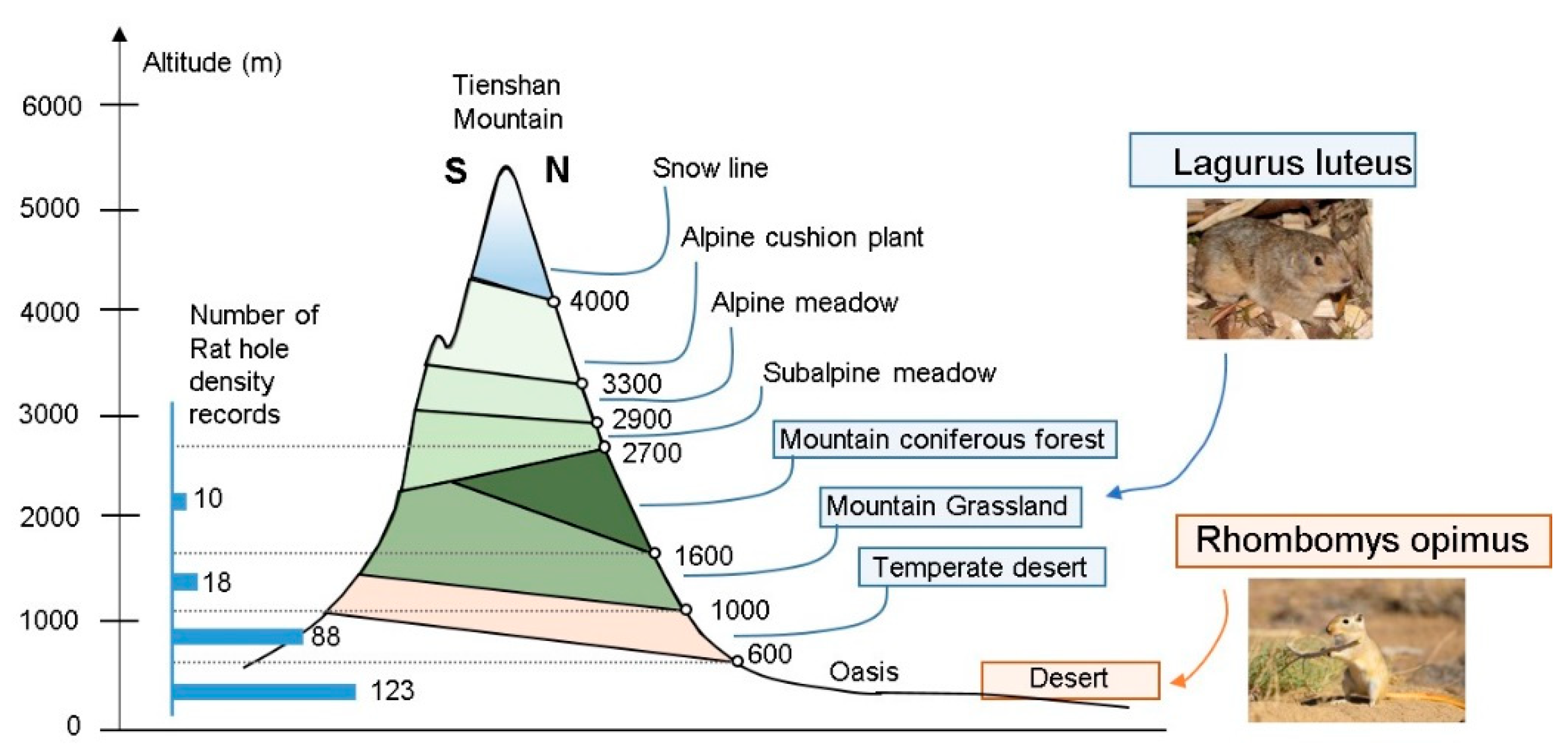
The northern slope of the Tien Shan Mountains belongs to a typical mountain–oasis–desert (from high land to low land) ecosystem [2,3] in the arid regions of Central Asia. The distribution of flora and fauna is strongly dependent on elevation variation. In NTXJ, rodent damage mainly occurs in grasslands and deserts and is primarily caused by Lagurus luteus (LL), which is mainly distributed in low mountain grassland, and Rhombomys opimus (RO), which is mainly distributed in the low desert. While the spatial and temporal distributions of RHD for both of these species are influenced by natural factors such as terrain [4], precipitation [5], temperature [6], soil texture [7,8], and vegetation [9], they may also be influenced by anthropogenic factors in the area, such as sheep grazing [10,11]. However, The temporal and spatial distribution of RHD and its complex driving mechanism remain uncertain. Although some ground in situ investigation and UAV-based approaches [4,12] have been used to measure the local or small-scale RHD within NTXJ and to analyze the relationships between RHD and environmental variables, there are numerous difficulties in extrapolating these local relationships to large-scale spatiotemporal mapping. The relationships between RHD and environmental variables’ data may vary by scale, which, for example, may be caused by the difference in the vegetation information provided at the field-scale of local studies and the pixel-scale of satellite remote sensing data. Additionally, the information provided by local studies is not sufficient for spatiotemporal mapping. Therefore, the lack of comprehensive analysis and modeling of the relationships between large-scale RHD and various environmental factors (both natural and anthropogenic) has limited the prospect of the spatiotemporal mapping of RHD (Figure 1). Satellite remote sensing data have been widely used to develop long-term large-scale datasets of vegetation such as the GIMMS NDVI product [13], meteorological data [14], and other variables, which may be effective in providing large-scale environmental factors’ data in the long time series. In addition, remote sensing data at the monthly scale may also help us understand the seasonal and monthly variation in the relationship between RHD and environmental factors. Further research in this area is crucial for the future prevention and control of damage caused by rodents.
Novel large-scale analysis and modeling may also be used to investigate the indirect interactions between RHD and ecosystems across elevation gradients. To date, machine learning approaches (e.g., random forest) have proven to be more effective in modeling the relationship between plant/animal communities and environmental factors [15] than traditional multiple regression analysis [16], especially when the volume of variables or data is large. They are also especially effective at estimating species distributions [17,18]. Bayesian network (BN) is a machine learning approach based on probability measures [19,20] that can quantify the complex, causal relationships between variables. This approach has advantages over other machine learning approaches in integrating expert knowledge and causal explanation. It can be used for probabilistic inference, diagnostic analysis, and decision support. BNs have also been used in species distribution studies [21] and proven effective in other ecological studies [22,23,24,25,26].
Our objective is to examine the relationship between RHD and ecosystems across elevation gradients and to determine their corresponding mechanisms when RHD and local conditions are influenced by the same environmental factors. This is particularly important to examine within NTXJ because local climate patterns have changed significantly [3], and precipitation in the mid-mountain region has increased due to oasis expansion and increased irrigation [27]. Thus, furthermore, the distribution and intensity of grazing may also be influenced by climate change and vegetation dynamics [28]. These environmental and anthropogenic factors can indirectly affect the large-scale distribution of RHD, but the spatial variability of these factors has rarely been considered in previous site-scale studies. Therefore, we analyzed the impacts of environmental factors on the large-scale RHD using satellite remote sensing data and BN. The training data are derived from in situ measured RHD investigations in NTXJ.

2. Methodology

2.1. Study Area

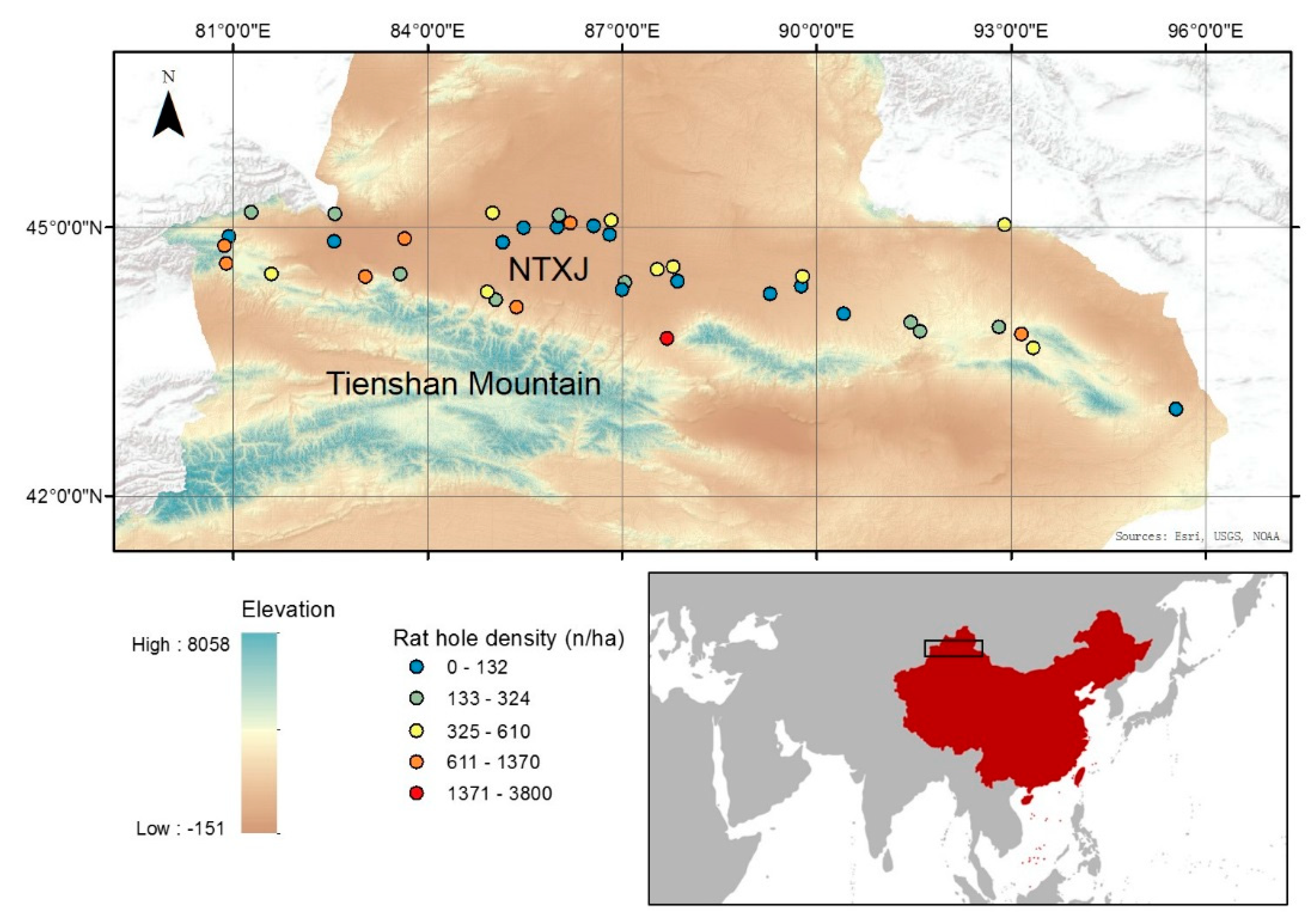
The terrain of NTXJ has a decreasing elevation gradient from the south (approximately 5000 m in the mountains) to the north (approximately 200 m at the edge of the desert) (Figure 2). The central region of NTXJ has a temperate continental arid climate, which is characterized by arid and hot summers and cold and windy winters. The annual average temperature ranges from <2 ℃ in the mountains to 8 to 10 ℃ in the plains. The precipitation season varies significantly, with the maximum precipitation concentrated in May and June, and the minimum amount in February. The annual precipitation gradually decreases from south to north, with annual precipitation in the southern mid-mountain region of 500 to 1000 mm, about 200 mm in the central plains, and about 100 mm in the northern desert [29]. The vertical distribution of its natural conditions (Figure 3) is a typical mountain-basin landform pattern. Different vertical elevation zones correspond to different landscape types and ecosystems. The unique natural conditions of NTXJ make it a typical representative of large-scale mountain–oasis–desert ecosystems in temperate arid regions of Central Asia [30].

2.2. Data

The data used in this study include published records of RHD in NTXJ and environmental factors. The RHD data were collected from published literature, which was mainly obtained from the China National Knowledge Infrastructure (CNKI) and in Chinese. We collected 239 RHD records with spatiotemporal information from published articles on the investigation of RHD within NTXJ. These records spanned from 1982 to 2015. Most of these raw data records were obtained from RHD surveys of small regions based on quadrats and UAV remote sensing. In addition to the temporal and spatial information of RHD, spatially averaged data of the environmental factors (Table 1) were extracted with raster data in each shapefile averaged in ArcGIS, including precipitation, temperature, soil texture, topography, shortwave radiation, and grazing intensity.

2.3. Bayesian Network

The BN [19] is a directed acyclic graph model. Its nodes represent the probability distribution of variables, and the directed edges represent the causal correlations given the conditional probability table. By combining prior knowledge and observational data, we obtain the conditional probability distribution of the network nodes. The expectation–maximization algorithm [36] is used to iteratively calculate the expectation and maximum likelihood estimation of the parameters and implement the optimization process for the missing data.
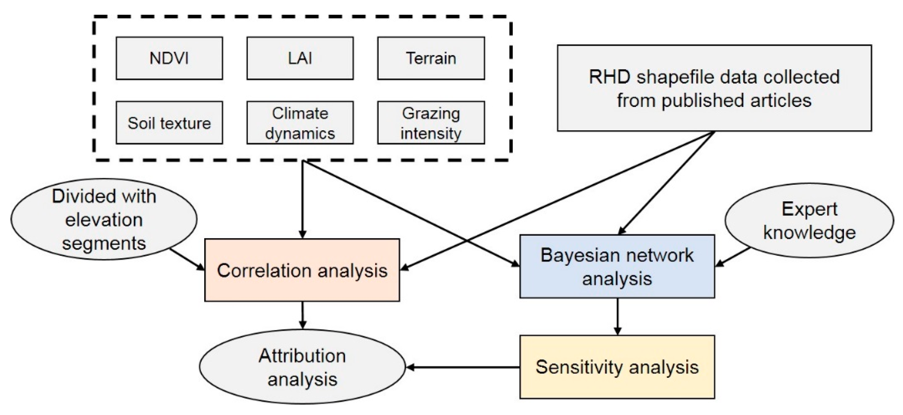
To simulate the causal relationship between RHD and environmental factors with a BN, we processed the multi-dimensional data collected from the articles into a training dataset with RHD as the target variables and environmental variables as the independent features (Figure 4). Based on empirical knowledge and preliminary correlation analysis, we chose suitable variables as nodes of BN and determined the directional causal link between nodes and the status discretization (Table 2) of each variable node to reduce the computational complexity of the joint probability distribution. The different numbers of intervals and segmentation points in the discretization process may have an impact on the performance of the model and the prior knowledge obtained from expert knowledge. Therefore, in this paper, the discretization of data was synchronized with the setting of prior knowledge, and expert knowledge and the actual data distribution guided the discretization procedure. Further, the BN was parameterized by the training data with the joint probability calculated.
A BN is composed of random variables (X1,., Xn) with their joint probability distribution [20] calculated as
P ( X ) = P ( X 1 , X 2 , , X n ) = i = 1 n P ( X i | pa ( X i ) )
where pa(Xi) is the value of the parent node of the child node Xi. With expert knowledge integrated, we can obtain the prior conditional probability table (CPT) of the BN. An expectation–maximization (EM) algorithm [36] was used to incorporate the observational data to calculate the posterior CPTs.
To evaluate the impacts of various environmental factors on RHD, we applied a sensitivity analysis based on mutual information (MI) [37,38]. This represents the entropy reduction in the child node given the status of the parent node. The higher the MI value is, the higher is the sensitivity of the child node to the parent node for the stronger causality. MI is calculated as follows:
MI = H ( Q ) - H ( Q | F ) = q f P ( q ,   f ) log 2 ( P ( q , f ) P ( q ) P ( f ) )  
where H represents the entropy, Q represents the target node, F represents the set of other nodes, and q and f represent the status of Q and F.
To understand the environmental driving mechanism of high RHD based on the built BN, we performed a diagnosis analysis [19] and obtained the posterior probability change in the environmental nodes given the specific status of the RHD node.

3. Results

3.1. Correlation Analysis of Environmental Factors Affecting RHD

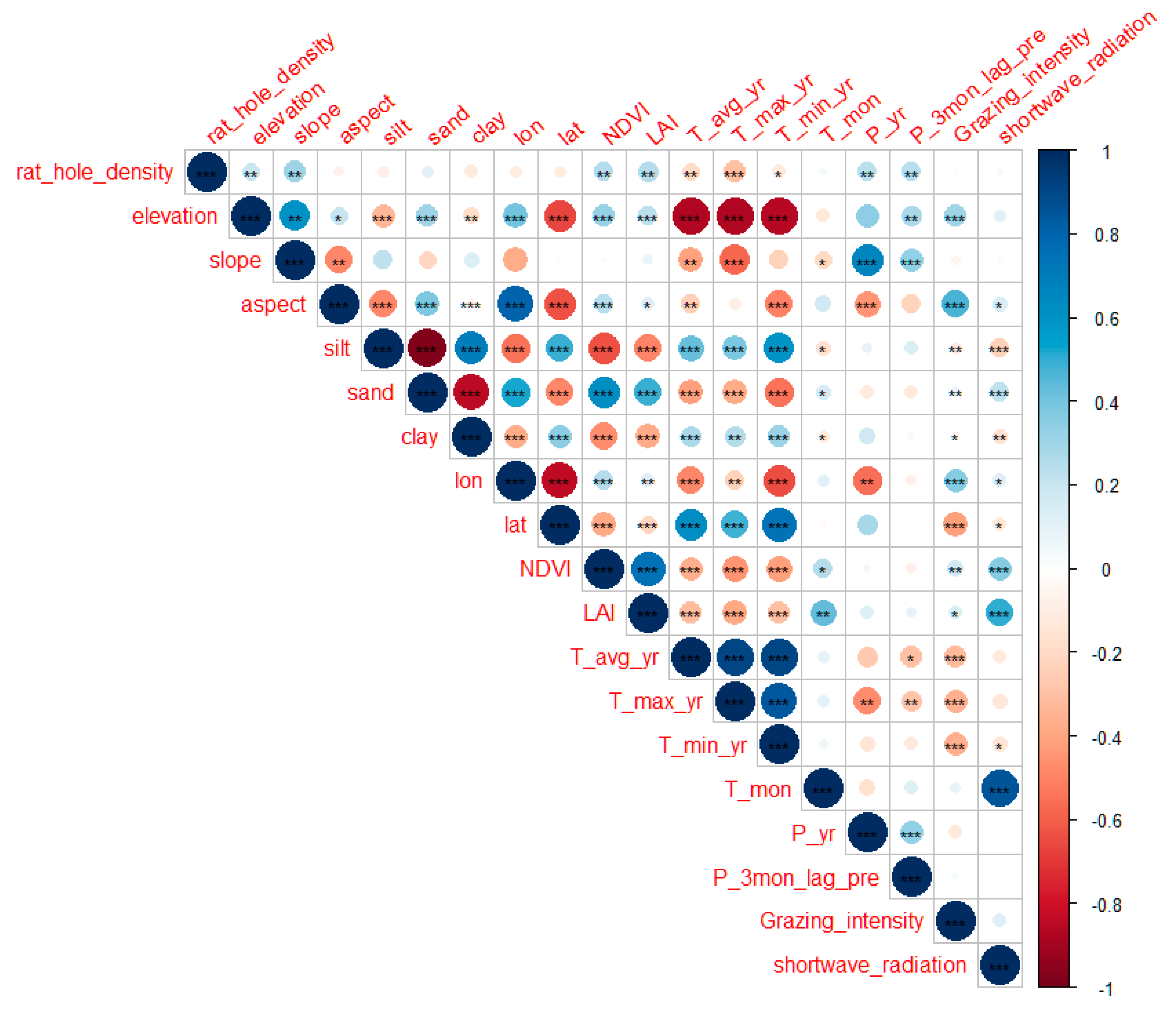
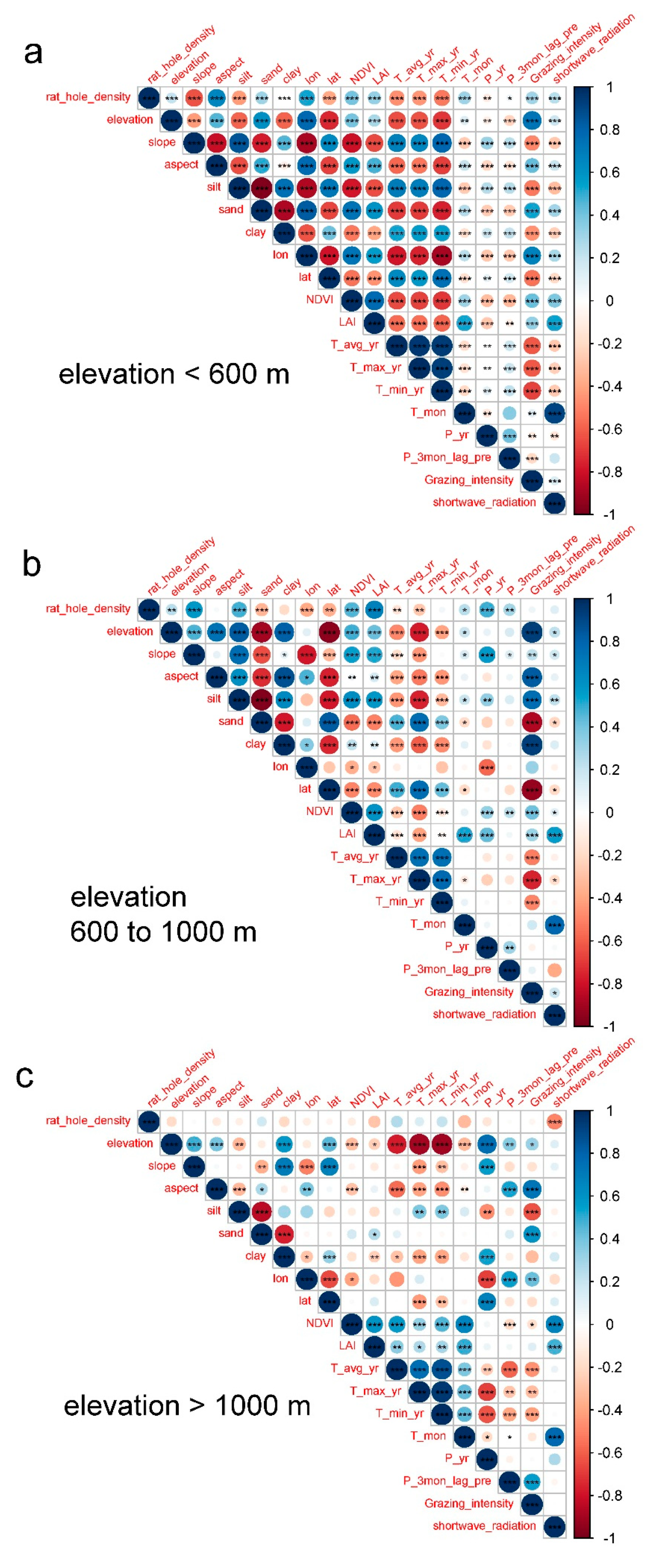
The correlation analysis (Figure 5) shows that RHD throughout NTXJ as a whole is significantly positively correlated with elevation, slope, NDVI, LAI, annual precipitation, and precipitation in the three months before the survey, and is significantly negatively correlated with temperature variables. However, based on the difference of the landscape divided by the elevation, the correlations show significant differences between regions with an elevation higher than 600 m (UPR) and regions with an elevation lower than 600 m (LWR) (Figure 6), while the correlations are mostly not significant with an elevation higher than 1000 m. In LWR, RHD is significantly correlated with most environmental variables. The seven main differences of the relationships between RHD and environmental variables in LWR and UPR include the following: (1) In LWR, RHD is significantly negatively correlated with slope, while in UPR, it is significantly positively correlated. This feature is just the opposite for aspect; (2) in LWR, RHD is significantly positively correlated with the sand content in the soil. This shows that RO may prefer to live in sandy areas. In UPR, the correlation is weak, possibly because the sand content is lower at higher altitudes; (3) in LWR, RHD has a significantly positive correlation with longitude, while in UPR, it has a significantly negative correlation; (4) in LWR, the negative correlation between RHD and temperature variables is stronger than in UPR; (5) in LWR, the positive correlation between RHD and precipitation is weaker than in UPR; (6) in LWR, RHD is significantly positively correlated with grazing intensity and shortwave radiation, while in UPR, the correlation is weak.

3.2. Sensitivity Analysis of Environmental Factors Affecting RHD Based on the BN

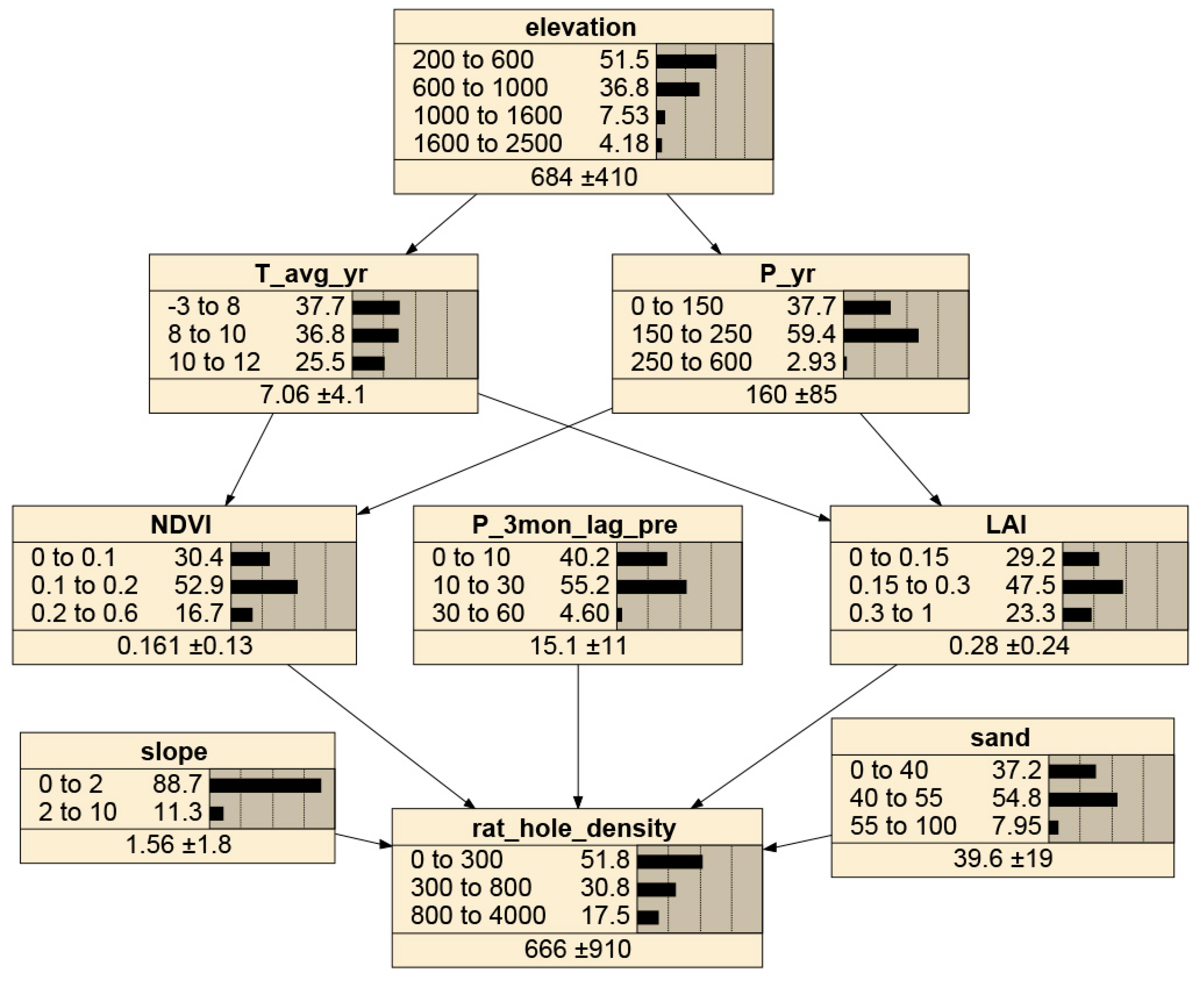
In addition to the linear correlation analysis above, the causal and individual impacts of these variables on RHD are not clear, due to the collinearity between environmental variables (e.g., in NTXJ, temperature and precipitation are highly correlated with elevation). The sensitivity analysis (Table 3) is based on the built BN (Figure 7) and shows that RHD throughout NTXJ as a whole is most sensitive to LAI, followed by NDVI, slope, and sand. The sensitivity of RHD to these variables shows significant differences in regions of various elevation ranges. The sensitivity of RHD to LAI is much higher in UPR than in LWR, which indicates that vegetation types at various elevation range significantly affect RHD. Furthermore, the sensitivity of RHD to NDVI above and below 600 m is not highly differentiated. It may be caused by the fact that the remote sensing NDVI data are not very effective in monitoring the growth and underground biomass of Haloxylon ammodendron, since RO takes the tender roots and twigs of Haloxylon ammodendron as the main food in the lower plain desert area of LWR. Moreover, in each elevation interval, the sensitivity of RHD to LAI is higher than that of NDVI. When compared with NDVI, LAI may be a better indicator of vegetation for measuring RHD in NTXJ.
In areas below an elevation of 1000 m, RHD is more sensitive to soil sand content. Without temporal variations, the soil sand content is primarily used to only explain the spatial variation of RHD. The sensitivity of RHD to soil sand content is even comparable to LAI; this is especially the case in LWR. This indicates that the distribution of RHD may be higher in areas with high sand content that are below the elevation of 1000 m. The sensitivity of RHD to the slope is highest in the range of 600 to 1000 m, followed by LWR, and lowest in areas above 1000 m. These findings indicate that the impacts of slope on RHD are limited to the low mountain regions and LWR.
However, an important consideration for these results is that the coarse-scale of the RHD data may not have captured the influence of small topographic characteristics throughout the study region. These findings may be impacted by the variation in the slope in conjunction with the variation of land cover types (from low mountain desert to oasis, to low plain desert), and as a result, RHD is more distributed in low mountain desert and plain desert. The sensitivity of RHD to annual precipitation is more sensitive in the elevation ranges of 600 m to 1000 m and 1000 m to 1600 m. This may be due to the high temporal and spatial heterogeneity of precipitation in these two altitude zones and the higher consequent impacts on vegetation growth. There is little difference across elevation ranges in the sensitivity of RHD to precipitation in the three months before each survey. RHD is more sensitive to the average annual temperature in LWR than in UPR, which may be because the vegetation condition of UPR is not as sensitive to temperature as that of LWR.

3.3. Causal Diagnosis of High RHD and Evaluation of the Potential Ecological Amplitude of Rats in LWR and UPR Based on the BN

Using the diagnostic analysis function of the BN, we analyzed the driving factors of severe and extremely severe rodent damage, which are determined by the high RHD (800 to 4000 n/ha) indirectly in LWR and UPR. As the high-value status of the RHD node is determined (Figure 8), the posterior probability distributions of other environmental variables consequently change (Table 4). In LWR, severe and extremely severe rodent damage is most likely caused in areas of medium soil sand content (+13.4%), high slope (+9.6%), and high LAI (+6.1%) when compared with the average level of rodent damage. In UPR, severe and extremely severe rodent damage is most likely to occur in areas of high NDVI (+16.2%), high LAI (+12.5%), high slope (+12.5%), and medium annual precipitation (+11.2%) when compared with the average level of rodent damage. Therefore, areas with the above environmental conditions may be the focus of future rodent damage control in NTXJ.

4. Discussion

4.1. The Effectiveness of a BN in the Attribution Analysis of RHD Distribution in NTXJ

Since BNs have been used extensively in ecological studies [23,24,25,26], especially for the expression of expert knowledge and cause and effect, it was an appropriate method for the attribution analysis of RHD in this study. The environmental variables used in this study inherently have a high linear correlation, so it was important to reduce the interference of collinearity between the variables. This enabled us to obtain a more accurate understanding of the effect of each environmental factor and to determine whether these factors directly or indirectly affect RHD. When compared with conventional correlation analysis or some non-causal machine learning methods such as random forest, a BN may have advantages in deepening the understanding of causal mechanisms because expert knowledge can be integrated. As ecosystem types in NTXJ are primarily determined, we focused on the vertical differentiation within various elevation ranges to be considered in the BN. Additionally, the dynamic diagnostic analysis function of the BN and the visualization of the ecological amplitude in this study enabled us to focus our analysis on the differential driving mechanisms of RHD under various environmental condition combinations. These results can enrich our knowledge and enable decision makers to make informed decisions regarding rodent damage control. Results derived from the BN can also be used for the probabilistic inference of RHD if environmental variables are given. These findings demonstrate the potential advantages of BN in decision support for rodent damage control.
However, a BN may also have limitations in studies such as this. One potential disadvantage is the lack of consideration of interaction relationships within the network. Since the relationship between BN nodes needs to be directional, some interaction relationships and feedbacks may be ignored [39]. For example, vegetation conditions affect the food sources of rats and thus affect RHD, but at the same time, high RHD will affect vegetation condition and soil physical–chemical properties [40,41]. Thus, the relationship between RHD and vegetation conditions may be reversed. If these relationships are not considered, our understanding of the interactive effects of vegetation and RHD may be limited. Furthermore, if the influence of predator populations, such as foxes [42], on RHD is included in this BN, the interaction relations will be more complicated and should thus not be ignored. Therefore, future studies should consider how to better incorporate the impacts of such interactions when such machine learning methods are used.

4.2. Uncertainties and Limitations Concerning the Driving Environmental Mechanisms of RHD in NTXJ

Previous studies have mostly analyzed small-scale and local RHD within NTXJ, but the study of large-scale RHD remains limited. The new findings of this study provide information in the quantitative relationship between large-scale RHD and environmental variables, and analyses on the different patterns of RHD across elevation ranges. Additionally, this study focused on the impacts of environmental factors on the temporal and spatial distribution of RHD, rather than the feedback of RHD on environmental factors (e.g., the impacts on vegetation degradation and soil texture) [43]. Our findings are constrained primarily by the directional limitation [39] between the BN nodes, but also because the environmental factor data obtained from the survey of surface soil texture may not be applicable to the feedback effect of RHD on local soil texture.
Given the results of the correlation analysis and the BN-based analysis, we found that vegetation condition is an important factor that affects the large-scale temporal and spatial distribution of RHD in NTXJ. Of all the other natural factors that were considered, this factor was significantly more important. This relationship can be attributed to the fact that vegetation is the most important food source for rats in NTXJ, and the temporal and spatial distribution of food sources heavily influences the distribution of rat populations. The differences in the relationships between RHD and LAI or NDVI may be influenced by the different types of vegetation that are consumed by RO in LWR and LL in UPR. Haloxylon ammodendron is the main food source for RO, whereas and LL primarily consumes Artemisia spp. Other factors (e.g., precipitation, temperature, grazing intensity) may also indirectly affect RHD through their effects on vegetation. However, the use of the coarser spatial resolution of NDVI and LAI data may bring uncertainty to such analyses, especially in desert areas with low vegetation coverage. This may lead to an underestimation of the impact of spatial vegetation variability on RHD. Due to the use of a monthly temporal resolution, the effects of temporal (i.e., interannual, seasonal) variability of the vegetation condition on RHD may have been considered to be a greater influence than the spatial variability. Furthermore, the 90 m resolution of terrain variables may not be a fine enough scale to capture the impacts of small-scale terrain factors (e.g., sand dunes with a scale below 20 m) on RHD [4]. In this case, the small-scale terrain factors obtained by UAV remote sensing [4] can be value-added because the extracted values from shady slopes and sunny slopes can be more accurate. Therefore, the guiding significance of the terrain-related variable analysis in this study for rodent damage control may only be effective at the regional scale, rather than the scale smaller than 90 m. In LWR, the major anthropogenic factor of grazing intensity is significantly positively correlated with RHD. One possible explanation for this relationship is that although grazing may threaten the food supply of RO, grazing in LWR occurs mostly in winter. This grazing period is staggered within the breeding season of RO (spring and summer), and the distribution of both RO and grazers depends on the synchronous distribution of vegetation. Thus, there may be positive correlation between grazing intensity and RDH. In UPR, the weak correlation between grazing intensity and RHD may be because grazing sheep do not feed on Artemisia spp. as their main food source, and the total vegetation in the area is sufficient for sheep and LL to coexist.
To predict the large-scale spatial and temporal distribution of rat population density, further considerations to the uncertainties and limitations should be made concerning the characteristics of the population. In this study, the seasonal changes in the rat population were mainly considered through the inclusion of monthly temporal variables (e.g., NDVI, temperature, and precipitation). However, for occasional occurrences of extremely high reproduction rates within the population, the predictive capability of these environmental variables may be limited significantly. Additionally, the sex ratio [6], age structure, and predator density for the rat population may also be important in predicting their density distribution. This should be a primary focus in future studies. These considerations may resolve the many limitations in generating accurate spatial and temporal maps of the rat density distribution. Likewise, more accurate environmental variable data, such as the distribution of Haloxylon ammodendron and other desert plants [44,45] is critical to predicting RHD distributions in the future.

4.3. Other Potential Impacts of Grazing on RHD

Although we found that grazing in LWR and UPR have had significantly different impacts on RHD, the nature of this conspecific relationship remains uncertain. This is because grazing intensity data that are purely based on statistical data cannot accurately represent the temporal and spatial dynamics of the past and present grazing systems and grassland management practices. The significant differences in water availability and vegetation conditions between LWR and UPR may dominate the impacts of grazing on RHD. One possible reason for the variable conditions between elevation zones is due to the joint effect of low water availability and photosynthate allocation in local vegetation. Under grazing conditions, the root–shoot ratio increases, and under conditions of low water availability, more photosynthate can be allocated to roots [46,47,48]. In LWR vegetation, more photosynthate may be allocated to roots to decrease transpiration under low water availability conditions. Likewise, the underground biomass of plants may also increase to adapt to the disturbance of grazing [49]. Therefore, more food resources can be provided for RO and may lead to a positive impact of grazing on RHD in LWR.
In UPR, grazing may reduce ET and increase soil moisture, which, in turn, promotes grass growth at certain grazing intensities [50]. Thus, the impact of grazing on RHD can be insignificant due to weak food competition between livestock and LL when there are sufficient food resources. However, under extreme drought conditions, water availability and food resources in UPR may also decrease significantly. Intensive grazing in the summer and autumn may greatly decrease the aboveground biomass throughout grassland areas and may further perpetuate the negative effects on RHD. Under these drought conditions, the plant biomass in LWR is also lower. This may result in decreased grazing intensity in winter and spring due to insufficient food resources provided, thus further influencing RHD in LWR. These considerations indicate that across areas of different water availability conditions, grazing systems may indirectly influence RHD in UPR and LWR across different elevation ranges. As RHD data collected in this study are limited to areas below alpine grassland at 2700 m, the impact of grazing on RHD in higher elevation areas is limited. However, these considerations may be not significant in NTXJ because the grazing duration on alpine grassland is short, lasting only one to two months, and is often concentrated in summer [50]. However, compared with NTXJ, throughout other alpine meadows, or grassland areas in the world [51,52,53], longer grazing durations may indeed have a more significant impact on the population density of rodents. In addition, in alpine meadows, small rodents such as pika may spend the winter by eating yak feces [54], so the population density and grazing intensity may also show a positive correlation.

4.4. The Prospect of Combining Satellite Remote Sensing Data and RHD Modeling

Compared with studies to identify local rat hole numbers, which may require very fine resolution such as UAV images, the main innovation of this research is to establish a relation between satellite remote sensing (e.g., NDVI data of GIMMS, DEM data of SRTM, and meteorological dataset made through a fusion of remote sensing products, reanalysis dataset and in situ observation data at weather stations) and the RHD in local-scale studies. This has rarely been reported in previous studies. This study proved the effectiveness of using large-scale satellite remote sensing data to analyze the temporal and spatial changes of the population density of rodents. In addition, the data used in this paper, such as soil texture, precipitation, temperature, etc., have other corresponding alternative datasets produced by satellite remote sensing. Therefore, in future studies, we can use various remote sensing datasets to establish a correlation with RHD. This is more suitable for large-scale rodent population monitoring. It may contribute to the application prospects of satellite remote sensing in animal ecology studies.

5. Conclusions

This study compiled small-scale and in situ RHD data in NTXJ that were collected between 1982 to 2015. Correlation analysis and BN were used to study the relationship between RHD and corresponding environmental variables. The conclusions are as follows:
1. The BN can effectively quantify causality in the environment-driven mechanism modeling of RHD in NTXJ and support decision making.
2. The NDVI and LAI data from satellite remote sensing are important to the spatial–temporal RHD distribution and the mapping in the future.
3. In LWR and UPR within NTXJ, there are significant, patterned differences in the driving mechanism of RHD, which are dependent on the elevation.
4. In LWR, vegetation conditions have weaker impacts on RHD than in UPR, possibly because of the Artemisia spp. eaten by LL in UPR is more sensitive to the spatial–temporal variations in precipitation and temperature than the Haloxylon ammodendron eaten by the RO in LWR.
5. In LWR, grazing intensity has a stronger positive correlation to RHD than in UPR, possibly because winter grazers and RO both depend on vegetation distribution. In UPR, sheep do not feed Artemisia spp. as the main food, and the total vegetation is sufficient for sheep and LL to coexist.
6. Under differing conditions of water availability in LWR and UPR, grazing may affect the ratio of aboveground and underground biomass through photosynthate allocation, thereby affecting the distribution of RHD. In extremely dry years, the RHD of LWR and UPR may have an indirect interactive relationship due to changes in grazing systems.

Author Contributions

Conceptualization, methodology, software, writing, H.S.; data curation, Q.P.; conceptualization and supervision, G.L.; methodology, O.H.; supervision and resources, C.C., T.V.d.V., A.K., P.D.M. and S.W. All authors have read and agreed to the published version of the manuscript.

Funding

This research has been supported by the High-End Foreign Experts Project, the Strategic Priority Research Programme of the Chinese Academy of Sciences (grant no. XDA23100000), National Science and Technology Basic Resources Survey Special Project (grant no.2017FY101004), the National Natural Science Foundation of China (grant nos. 41671108), and the Chinese Academy of Sciences President’s International Fellowship Initiative (PIFI) (grant no. 2017VCA0002).

Data Availability Statement

Data used in this study are available upon reasonable request to the first author Haiyang Shi ([email protected]).

Conflicts of Interest

The authors declare that they have no known competing financial interests or personal relationships that could have appeared to influence the work reported in this paper.

References

  1. Yang, W.; Jiang, H.; Wang, X.; XU, W. Disturbance Effects of Rhombomys Opimus on Desert Plant Community in Gurbantonggut Desert. Chin. J. Ecol. 2009, 28, 2020–2025. [Google Scholar]
  2. Luo, G.; Feng, Y.; Zhang, B.; Cheng, W. Sustainable Land-Use Patterns for Arid Lands: A Case Study in the Northern Slope Areas of the Tianshan Mountains. J. Geogr. Sci. 2010, 20, 510–524. [Google Scholar] [CrossRef]
  3. Zhang, M.; Luo, G.; Cao, X.; Hamdi, R.; Li, T.; Cai, P.; Ye, H.; He, H. Numerical Simulation of the Irrigation Effects on Surface Fluxes and Local Climate in Typical Mountain-oasis-desert Systems in the Central Asia Arid Area. J. Geophys. Res. Atmos. 2019, 124, 12485–12506. [Google Scholar] [CrossRef]
  4. Wen, A.; Zheng, J.; Chen, M.; Mu, C.; Tao, M. Spatial Distribution of Rodent Pests in Desert Forest Based on UAV Remote Sensing. In Proceedings of the 2016 IEEE International Geoscience and Remote Sensing Symposium (IGARSS), Beijing, China, 10–15 July 2016; pp. 1804–1807. [Google Scholar]
  5. Tianbiao, Z.; Chi, Y.; Lizhi, Z.; Zhongbing, Z.; Feihu, J.; Jianping, W.; Shulong, N. Relationship between Population Density and Rainfall in Great Gerbil (Rhombomys Opimus). Acta Theriol. Sin. 2007, 27, 195–199. [Google Scholar]
  6. Randall, J.A.; Rogovin, K.; Parker, P.G.; Eimes, J.A. Flexible Social Structure of a Desert Rodent, Rhombomys Opimus: Philopatry, Kinship, and Ecological Constraints. Behav. Ecol. 2005, 16, 961–973. [Google Scholar] [CrossRef] [Green Version]
  7. Prakash, I.; Ghosh, P.K. Rodents in Desert Environments; Springer Science & Business Media: Berlin/Heidelberg, Germany, 2012; Volume 28, ISBN 94-010-1944-4. [Google Scholar]
  8. Randall, J.A. Behavioural Adaptations of Desert Rodents (Heteromyidae). Anim. Behav. 1993, 45, 263–287. [Google Scholar] [CrossRef] [Green Version]
  9. Mares, M.A.; Ojeda, R.A.; Borghi, C.E.; Giannoni, S.M.; Diaz, G.B.; Braun, J.K. How Desert Rodents Overcome Halophytic Plant Defenses. BioScience 1997, 47, 699–704. [Google Scholar] [CrossRef]
  10. Han, Q.; Luo, G.; Li, C.; Shakir, A.; Wu, M.; Saidov, A. Simulated Grazing Effects on Carbon Emission in Central Asia. Agric. For. Meteorol. 2016, 216, 203–214. [Google Scholar] [CrossRef]
  11. Huang, X.; Luo, G.; Han, Q. Temporospatial Patterns of Human Appropriation of Net Primary Production in Central Asia Grasslands. Ecol. Indic. 2018, 91, 555–561. [Google Scholar] [CrossRef]
  12. Amin, W.; JiangHua, Z.; Meng, C.; Chen, M.; Tao, M. Monitoring mouse-hole density by Rhombomys opimus in desert forests with UAV remote sensing technology. Sci. Silvae Sin. 2018, 54, 186–192. [Google Scholar]
  13. The National Center for Atmospheric Research Global GIMMS NDVI3g v1 Dataset (1981–2015); National Tibetan Plateau Data Center: Beijing, China, 2018.
  14. Yang, K.; He, J. China Meteorological Forcing Dataset (1979—2018); National Tibetan Plateau Data Center: Beijing, China, 2019. [Google Scholar]
  15. Baltensperger, A.P.; Huettmann, F. Predictive Spatial Niche and Biodiversity Hotspot Models for Small Mammal Communities in Alaska: Applying Machine-Learning to Conservation Planning. Landsc. Ecol 2015, 30, 681–697. [Google Scholar] [CrossRef]
  16. Melis, C.; Szafrańska, P.A.; Jędrzejewska, B.; Bartoń, K. Biogeographical Variation in the Population Density of Wild Boar (Sus Scrofa) in Western Eurasia. J. Biogeogr. 2006, 33, 803–811. [Google Scholar] [CrossRef]
  17. Fischer, C.; Schröder, B. Predicting Spatial and Temporal Habitat Use of Rodents in a Highly Intensive Agricultural Area. Agric. Ecosyst. Environ. 2014, 189, 145–153. [Google Scholar] [CrossRef]
  18. Wiersma, Y.F.; Huettmann, F.; Drew, C.A. Introduction. Landscape Modeling of Species and Their Habitats: History, Uncertainty, and Complexity. In Predictive Species and Habitat Modeling in Landscape Ecology: Concepts and Applications; Drew, C.A., Wiersma, Y.F., Huettmann, F., Eds.; Springer: New York, NY, USA, 2011; pp. 1–6. ISBN 978-1-4419-7390-0. [Google Scholar]
  19. Friedman, N.; Geiger, D.; Goldszmidt, M. Bayesian Network Classifiers. Mach. Learn. 1997, 29, 131–163. [Google Scholar] [CrossRef] [Green Version]
  20. Pearl, J. Bayesian Netwcrks: A Model Cf Self-Activated Memory for Evidential Reasoning. In Proceedings of the 7th Conference of the Cognitive Science Society, University of California, Irvine, CA, USA, 15–17 August 1985; pp. 15–17. [Google Scholar]
  21. Aguilera, P.A.; Fernández, A.; Reche, F.; Rumí, R. Hybrid Bayesian Network Classifiers: Application to Species Distribution Models. Environ. Model. Softw. 2010, 25, 1630–1639. [Google Scholar] [CrossRef]
  22. Albuquerque, M.T.D.; Gerassis, S.; Sierra, C.; Taboada, J.; Martín, J.E.; Antunes, I.M.H.R.; Gallego, J.R. Developing a New Bayesian Risk Index for Risk Evaluation of Soil Contamination. Sci. Total Environ. 2017, 603–604, 167–177. [Google Scholar] [CrossRef]
  23. Couture, R.-M.; Moe, S.J.; Lin, Y.; Kaste, Ø.; Haande, S.; Lyche Solheim, A. Simulating Water Quality and Ecological Status of Lake Vansjø, Norway, under Land-Use and Climate Change by Linking Process-Oriented Models with a Bayesian Network. Sci. Total Environ. 2018, 621, 713–724. [Google Scholar] [CrossRef] [PubMed]
  24. McCann, R.K.; Marcot, B.G.; Ellis, R. Bayesian Belief Networks: Applications in Ecology and Natural Resource Management. Can. J. For. Res. 2006, 36, 3053–3062. [Google Scholar] [CrossRef]
  25. Milns, I.; Beale, C.M.; Smith, V.A. Revealing Ecological Networks Using Bayesian Network Inference Algorithms. Ecology 2010, 91, 1892–1899. [Google Scholar] [CrossRef]
  26. Trifonova, N.; Kenny, A.; Maxwell, D.; Duplisea, D.; Fernandes, J.; Tucker, A. Spatio-Temporal Bayesian Network Models with Latent Variables for Revealing Trophic Dynamics and Functional Networks in Fisheries Ecology. Ecol. Inform. 2015, 30, 142–158. [Google Scholar] [CrossRef] [Green Version]
  27. Cai, P.; Hamdi, R.; Luo, G.; He, H.; Zhang, M.; Termonia, P.; De Maeyer, P. Agriculture Intensification Increases Summer Precipitation in Tianshan Mountains, China. Atmos. Res. 2019, 227, 140–146. [Google Scholar] [CrossRef]
  28. Liao, C.; Morreale, S.J.; Kassam, K.-A.S.; Sullivan, P.J.; Fei, D. Following the Green: Coupled Pastoral Migration and Vegetation Dynamics in the Altay and Tianshan Mountains of Xinjiang, China. Appl. Geogr. 2014, 46, 61–70. [Google Scholar] [CrossRef]
  29. Zhang, W.; Luo, G.; Chen, C.; Ochege, F.U.; Hellwich, O.; Zheng, H.; Hamdi, R.; Wu, S. Quantifying the Contribution of Climate Change and Human Activities to Biophysical Parameters in an Arid Region. Ecol. Indic. 2021, 129, 107996. [Google Scholar] [CrossRef]
  30. Shi, H.; Luo, G.; Zheng, H.; Chen, C.; Hellwich, O.; Bai, J.; Liu, T.; Liu, S.; Xue, J.; Cai, P.; et al. A Novel Causal Structure-Based Framework for Comparing a Basin-Wide Water–Energy–Food–Ecology Nexus Applied to the Data-Limited Amu Darya and Syr Darya River Basins. Hydrol. Earth Syst. Sci. 2021, 25, 901–925. [Google Scholar] [CrossRef]
  31. CGIAR-CSI SRTM DEM Dataset in China (2000); National Tibetan Plateau Data Center: Beijing, China, 2013.
  32. Shouzhang Peng 1-Km Monthly Precipitation Dataset for China (1901–2017); National Tibetan Plateau Data Center: Beijing, China, 2020.
  33. Shouzhang Peng 1-Km Monthly Mean Temperature Dataset for China (1901–2017); National Tibetan Plateau Data Center: Beijing, China, 2019.
  34. Shouzhang Peng 1-Km Monthly Maximum Temperature Dataset for China (1901–2017); National Tibetan Plateau Data Center: Beijing, China, 2020.
  35. Shouzhang Peng 1-Km Monthly Minimum Temperature Dataset for China (1901–2017); National Tibetan Plateau Data Center: Beijing, China, 2020.
  36. Moon, T.K. The Expectation-Maximization Algorithm. IEEE Signal Process. Mag. 1996, 13, 47–60. [Google Scholar] [CrossRef]
  37. Castillo, E.; Gutiérrez, J.M.; Hadi, A.S. Sensitivity Analysis in Discrete Bayesian Networks. IEEE Trans. Syst. Man Cybern.-Part A Syst. Hum. 1997, 27, 412–423. [Google Scholar] [CrossRef] [Green Version]
  38. Laskey, K.B. Sensitivity Analysis for Probability Assessments in Bayesian Networks. IEEE Trans. Syst. Man Cybern. 1995, 25, 901–909. [Google Scholar] [CrossRef] [Green Version]
  39. Marcot, B.G.; Penman, T.D. Advances in Bayesian Network Modelling: Integration of Modelling Technologies. Environ. Model. Softw. 2019, 111, 386–393. [Google Scholar] [CrossRef]
  40. Xiang, Y.; Wang, Z.; Lyu, X.; He, Y.; Li, Y.; Zhuang, L.; Zhao, W. Effects of Rodent-Induced Disturbance on Eco-Physiological Traits of Haloxylon Ammodendron in the Gurbantunggut Desert, Xinjiang, China. J. Arid Land 2020, 12, 508–521. [Google Scholar] [CrossRef]
  41. Xu, W.; Liu, W.; Yang, W.; Wang, M.; Xu, F.; Blank, D. Impact of Great Gerbils (Rhombomys Opimus) on Desert Plant Communities. J. Arid Land 2015, 7, 852–859. [Google Scholar] [CrossRef] [Green Version]
  42. Wen, X.; Cheng, X.; Dong, Y.; Wang, Q.; Lin, X. Analysis of the Activity Rhythms of the Great Gerbil (Rhombomys Opimus) and Its Predators and Their Correlations Based on Infrared Camera Technology. Glob. Ecol. Conserv. 2020, 24, e01337. [Google Scholar] [CrossRef]
  43. Yoshihara, Y.; Okuro, T.; Buuveibaatar, B.; Undarmaa, J.; Takeuchi, K. Complementary Effects of Disturbance by Livestock and Marmots on the Spatial Heterogeneity of Vegetation and Soil in a Mongolian Steppe Ecosystem. Agric. Ecosyst. Environ. 2010, 135, 155–159. [Google Scholar] [CrossRef]
  44. Li, J.; Chang, H.; Liu, T.; Zhang, C. The Potential Geographical Distribution of Haloxylon across Central Asia under Climate Change in the 21st Century. Agric. For. Meteorol. 2019, 275, 243–254. [Google Scholar] [CrossRef]
  45. Tao, Y.; Wu, G.-L.; Zhang, Y.-M. Dune-Scale Distribution Pattern of Herbaceous Plants and Their Relationship with Environmental Factors in a Saline–Alkali Desert in Central Asia. Sci. Total Environ. 2017, 576, 473–480. [Google Scholar] [CrossRef] [PubMed]
  46. McConnaughay, K.D.M.; Coleman, J.S. Biomass Allocation in Plants: Ontogeny or Optimality? A Test Along Three Resource Gradients. Ecology 1999, 80, 2581–2593. [Google Scholar] [CrossRef]
  47. Ngugi, M.R.; Hunt, M.A.; Doley, D.; Ryan, P.; Dart, P. Dry Matter Production and Allocation in Eucalyptus Cloeziana and Eucalyptus Argophloia Seedlings in Response to Soil Water Deficits. New For. 2003, 26, 187–200. [Google Scholar] [CrossRef]
  48. Xu, Z.-Z.; Zhou, G.-S. Effects of Water Stress and Nocturnal Temperature on Carbon Allocation in the Perennial Grass, Leymus Chinensis. Physiol. Plant. 2005, 123, 272–280. [Google Scholar] [CrossRef]
  49. Frank, D.A.; Kuns, M.M.; Guido, D.R. Consumer Control of Grassland Plant Production. Ecology 2002, 83, 602–606. [Google Scholar] [CrossRef]
  50. Luo, G.; Han, Q.; Zhou, D.; Li, L.; Chen, X.; Li, Y.; Hu, Y.; Li, B.L. Moderate Grazing Can Promote Aboveground Primary Production of Grassland under Water Stress. Ecol. Complex. 2012, 11, 126–136. [Google Scholar] [CrossRef]
  51. Eldridge, D.J.; Travers, S.K.; Val, J.; Zaja, A.; Veblen, K.E. Horse Activity Is Associated with Degraded Subalpine Grassland Structure and Reduced Habitat for a Threatened Rodent. Rangel. Ecol. Manag. 2019, 72, 467–473. [Google Scholar] [CrossRef]
  52. Morgia, V.L.; Balbo, C.; Memoli, S.; Isaia, M. Rodents in Grassland Habitats: Does Livestock Grazing Matter? A Comparison of Two Alpine Sites with Different Grazing Histories. Zoos 2015, 37, 571–580. [Google Scholar] [CrossRef] [Green Version]
  53. Wang, Y.; Zhang, X.; Sun, Y.; Chang, S.; Wang, Z.; Li, G.; Hou, F. Pika Burrow and Zokor Mound Density and Their Relationship with Grazing Management and Sheep Production in Alpine Meadow. Ecosphere 2020, 11, e03088. [Google Scholar] [CrossRef]
  54. Speakman, J.R.; Chi, Q.; Ołdakowski, Ł.; Fu, H.; Fletcher, Q.E.; Hambly, C.; Togo, J.; Liu, X.; Piertney, S.B.; Wang, X.; et al. Surviving Winter on the Qinghai-Tibetan Plateau: Pikas Suppress Energy Demands and Exploit Yak Feces to Survive Winter. Proc. Natl. Acad. Sci. USA 2021, 118. [Google Scholar] [CrossRef] [PubMed]
Figure 1. Conventional field-scale investigation of RHD and analysis (a) and prospect toward the large-scale spatiotemporal RHD mapping and the analysis of the impacts of environmental factors (b).
Remotesensing 13 04709 g001
Figure 2. The location of the study area NTXJ (on the northern slope of Tien Shan Mountains in Xinjiang, China) and the spatial distribution of the collected rat hole density data in this study. This map is made based on the base map service GS (2016)1613 of China.
Remotesensing 13 04709 g002
Figure 3. Vertical distribution of the vegetation types and the numbers of the collected rat hole density (n/ha) records on the northern slope of Tien Shan Mountains at Bogda Peak section. Different vertical elevation zones correspond to different landscape types and ecosystems.
Remotesensing 13 04709 g003
Figure 4. Flowchart of the analysis.
Remotesensing 13 04709 g004
Figure 5. Correlation coefficient matrix of factors affecting rat hole density throughout NTXJ. (***), (**), and (*) represent the significance level of p-value < 0.01, 0.05, and 0.1, respectively.
Remotesensing 13 04709 g005
Figure 6. Correlation coefficient matrix of the factors affecting rat hole density in plain deserts with an elevation lower than 600 m (a), low mountain temperate deserts with an elevation of 600 m to 1000 m (b), and mountain grasslands with an elevation higher than 1000 m (c). (***), (**), and (*) represent the significance level of p-value < 0.01, 0.05, and 0.1, respectively.
Remotesensing 13 04709 g006
Figure 7. The Bayesian network of causality among natural environmental factors influencing rat hole density. In each node, the black histogram represents the probability distribution, the values before and after the “±” indicate the mean and standard deviation of the distribution, respectively.
Remotesensing 13 04709 g007
Figure 8. The BN-based diagnostic analysis of the occurrence of high RHD (800 to 4000 n/ha) in LWR (a) and UPR (b). The values before and after the “±” indicate the mean and standard deviation of the distribution, respectively.
Remotesensing 13 04709 g008
Table 1. Description of data on environmental factors that affect RHD.
Environmental FactorsExplanationRaw Dataset SourceSpatiotemporal Resolution
Elevation SRTM DEM dataset in China (2000) [31]90 m
Slope SRTM DEM dataset in China (2000) [31]90 m
Aspect SRTM DEM dataset in China (2000) [31]90 m
SandPercentage of sand content in topsoilHarmonized World Soil Database
SiltPercentage of silt content in topsoilHarmonized World Soil Database
ClayPercentage of clay content in topsoilHarmonized World Soil Database
P_yrAnnual precipitation1 km monthly precipitation dataset for China (1901–2017) [32]. The dataset was made through a fusion of remote sensing products, a reanalysis dataset, and in situ observation data at weather stations.1 km, yearly
P_3mon_lag_prePrecipitation in the three months before the survey1 km monthly precipitation dataset for China (1901–2017) [32]1 km, monthly
T_avg_yrAnnual average temperature1 km monthly mean temperature dataset for china (1901–2017) [33]1 km, yearly
T_max_yrMonthly maximum temperature1 km monthly maximum temperature dataset for China (1901–2017) [34]1 km, monthly
T_min_yrMonthly minimum temperature1 km monthly minimum temperature dataset for China (1901–2017) [35]1 km, monthly
T_monMonthly average temperature1 km monthly mean temperature dataset for china (1901–2017) [33]1 km, monthly
NDVINormalized vegetation indexNOAA Global Inventory Monitoring and Modeling System (GIMMS), version number 3g.v18 km, monthly (Maximum Value Composites with 15-day raw data) from 1981 to 2015
LAILeaf area indexNOAA Climate Data Record (CDR) of Leaf Area Index (LAI) and Fraction of Absorbed Photosynthetically Active Radiation (FAPAR), Version 48 km, monthly (mean value of daily raw data) from 1982 through the present
Grazing intensityGrazing intensity (number of livestock per hectare)FAO (http://www.fao.org/livestock-systems/en/, last accessed: 10 November 2021), field data in 2015, Xinjiang statistical yearbook [10,11]0.08333°, yearly
Shortwave radiation China meteorological forcing dataset (1979–2018) [14]0.1°, monthly (mean value of 3-hour raw data)
Table 2. Discretization of the status of the included variables as nodes of the BN.
VariablesStatus LevelsUnit
RHD0 to 300, 300 to 800, 800 to 4000n/ha
Elevation200 to 600, 600 to 1000, 1000 to 1600, 1600 to 2500m
P_yr0 to 150, 150 to 250, 250 to 600mm
T_avg_yr−3 to 8, 8 to 10, 10 to 12°C
P_3mon_lag_pre0 to 10, 10 to 30, 30 to 60mm
NDVI0 to 0.1, 0.1 to 0.2, 0.2 to 0.6
LAI0 to 0.15, 0.15 to 0.3, 0.3 to 1
Slope0 to 2, 2 to 10°
Sand0 to 40, 40 to 55, 55 to 100
Table 3. Sensitivity of RHD to environmental variables for the whole NTXJ and the subregions divided by elevation.
Environmental VariablesNTXJPlain Desert (200 to 600 m)Desert & low Mountain (600 to 1000 m)Grassland & Low Mountain (1000 to 1600 m)Grassland/Coniferous Forest & Mid Mountain(1600 to 2500 m)
Elevation0.01215no valueno valueno valueno value
LAI0.064450.035610.082590.075750.08313
NDVI0.039740.027370.057080.015350.00865
Sand0.024470.035860.028400.004770.00398
Slope0.026980.021630.050880.004810.00454
P_yr0.014920.002360.020170.022460.00046
P_3mon_lag_pre0.010620.011600.014050.008070.01112
T_avg_yr0.007390.009120.0014200
Table 4. Potential changes in the probability of the status of environmental variables corresponding to the occurrence of high RHD (800 to 4000 n/ha) in LWR and UPR.
Environmental VariablesProbabilistic Changes in the Status of Environmental Variables Due to the Determination of the High RHD Status in LWR (%)Probabilistic Changes in the Status of Environmental Variables Due to the Determination of the High RHD Status in UPR (%)
LowMediumHighLowMediumHigh
LAI+2.6−8.7+6.1−0.5−12.0+12.5
NDVI+5.6−11.6+6.0+1.8−18.0+16.2
Sand−17.9+13.4+4.5−6.5+3.2+3.3
Slope−9.6no value+9.6−12.5no value+12.5
P_yr−2.8+2.80−12.8+11.2+1.6
P_3mon_lag_pre−5.5+3.4+2.1−5.5+2.8+2.7
T_avg_yr+1.1−0.5−0.6+3.7−3.70
Note: “low”, “medium”, and “high” represent the low-, medium-, and high-value status of the nodes, respectively.
Publisher’s Note: MDPI stays neutral with regard to jurisdictional claims in published maps and institutional affiliations.