
Accurate Localization of Oil Tanks in Remote Sensing Images via FGMRST-Based CNN

 ,
,
Abstract
:1. Introduction
2. Methods
2.1. CNN-Based Localization Method of the Oil Tank
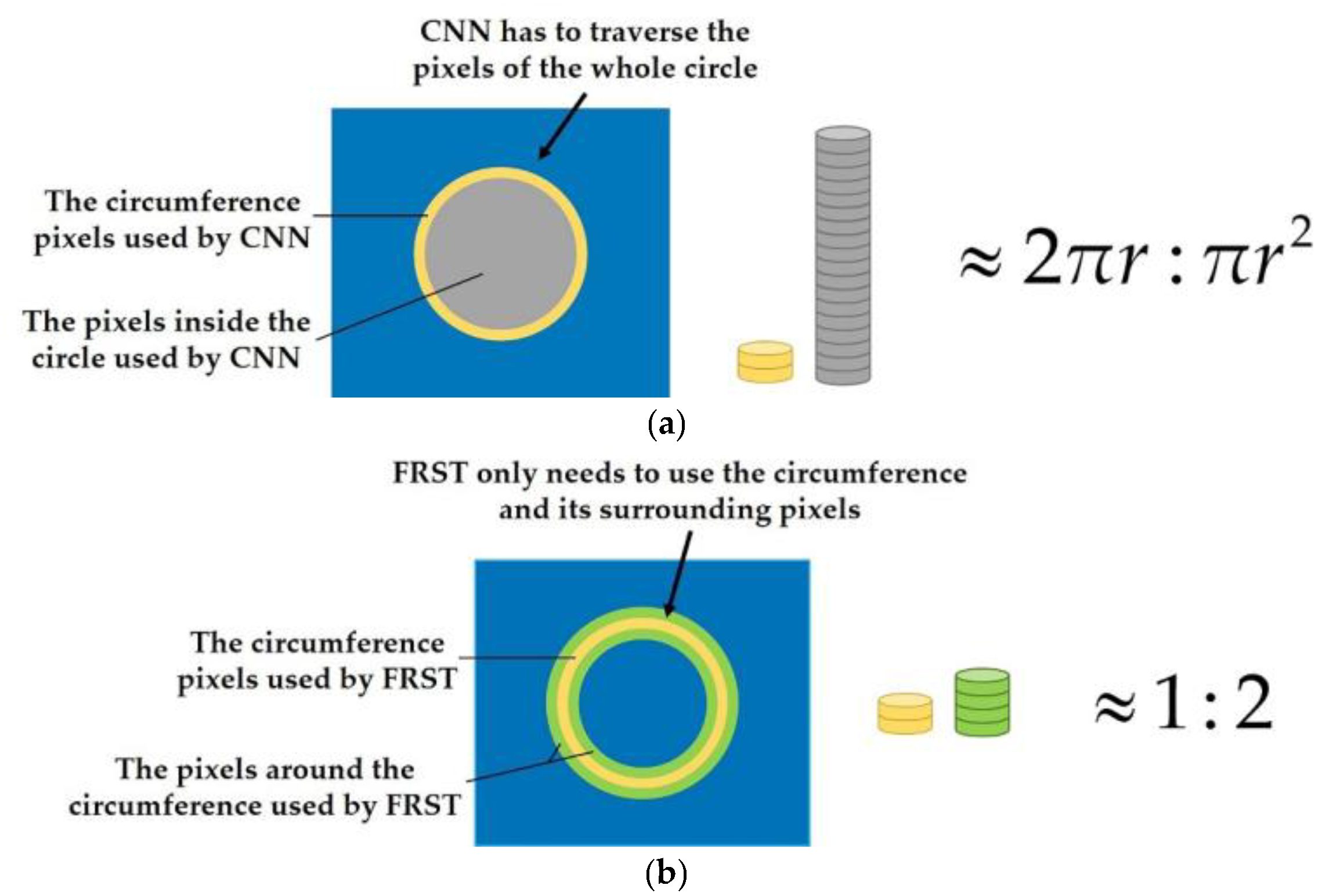
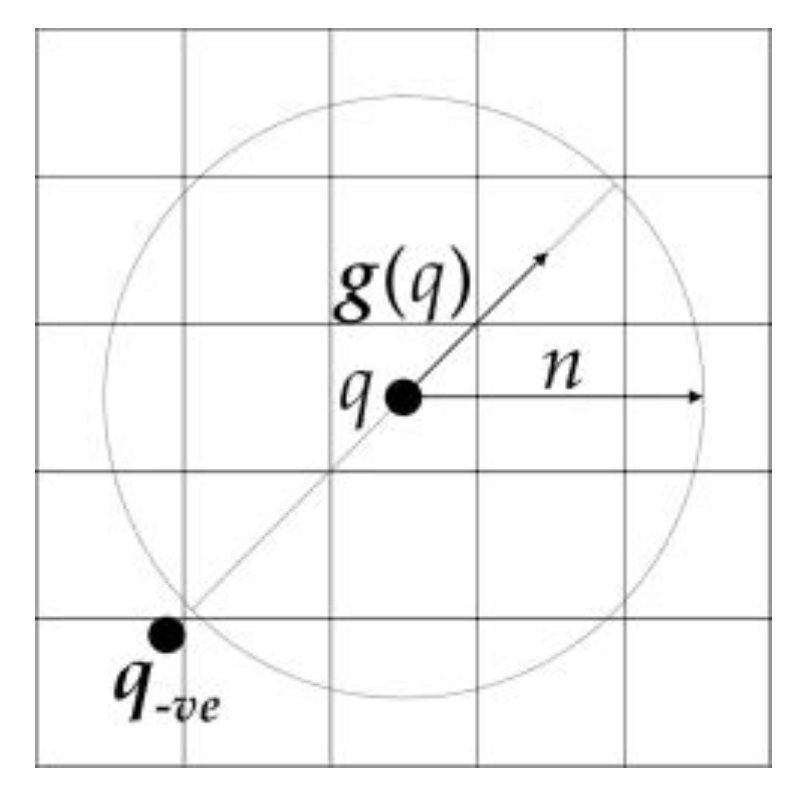
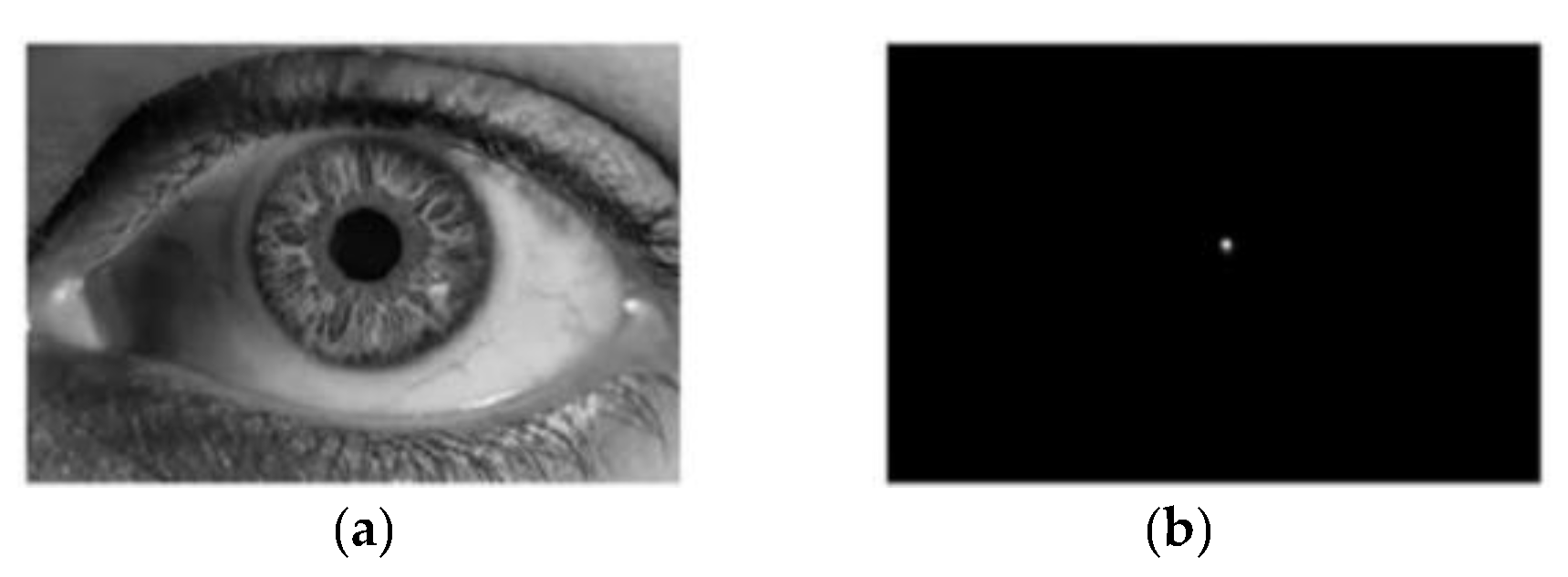
- The main feature of an object with a circular structure such as the oil tank is on the circumference, but not in the circle (as shown in Figure 1). However, at present, the neural networks need to traverse all the pixels (as shown in Figure 2a), which leads to a large increase in unnecessary computation and a low processing efficiency.
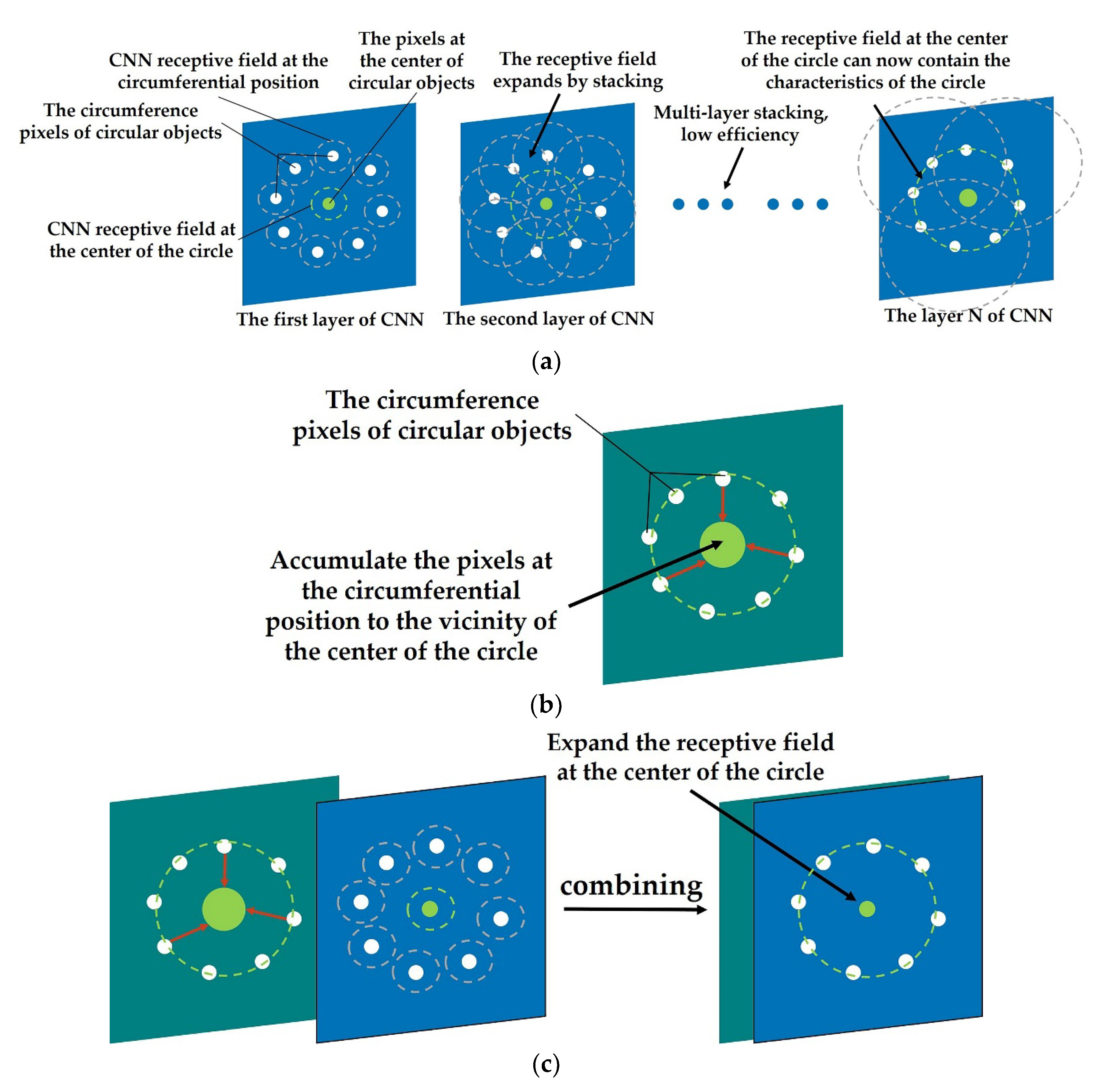
- Due to the limitation of the receptive field, CNN gradually increases the receptive field and aggregates the spatial features by cascading networks (as shown in Figure 3a). Therefore, the larger the object size is, the deeper the network structure is required, which leads to a large number of parameters and computation.
- It depends on the abundance and quantity of training samples, which does not exist in the traditional parameterized feature extraction method.
2.2. FGMRST-Based Localization Method of the Oil Tank
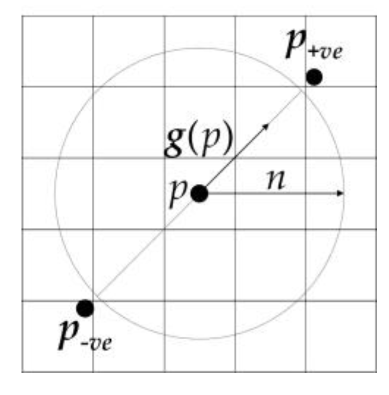
2.2.1. Introduction of FRST Theory
2.2.2. An Improved FRST Algorithm Based on the Characteristics of Oil Tank Images—FGMRST
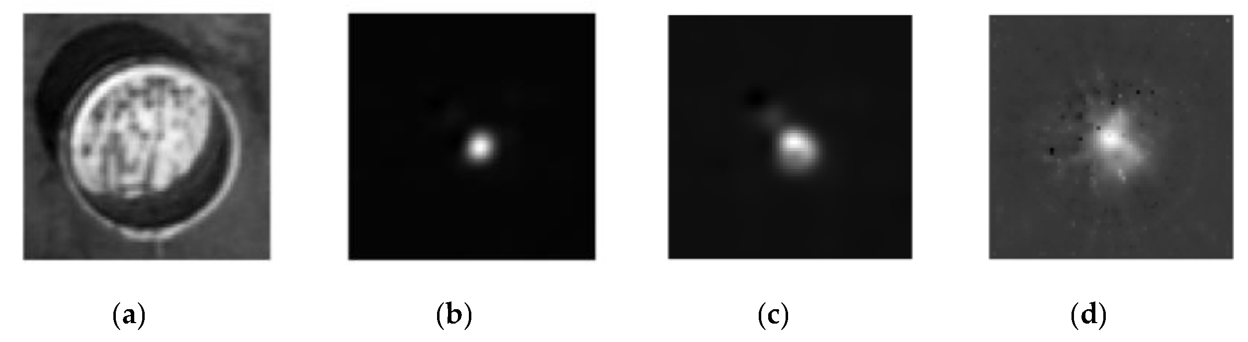
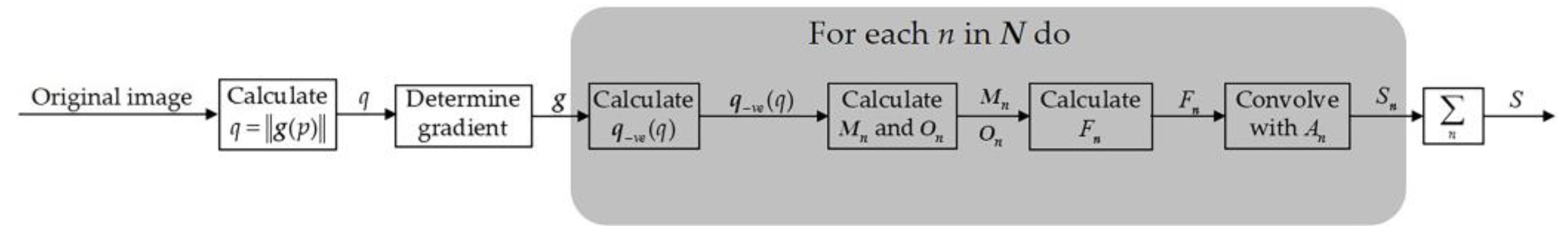
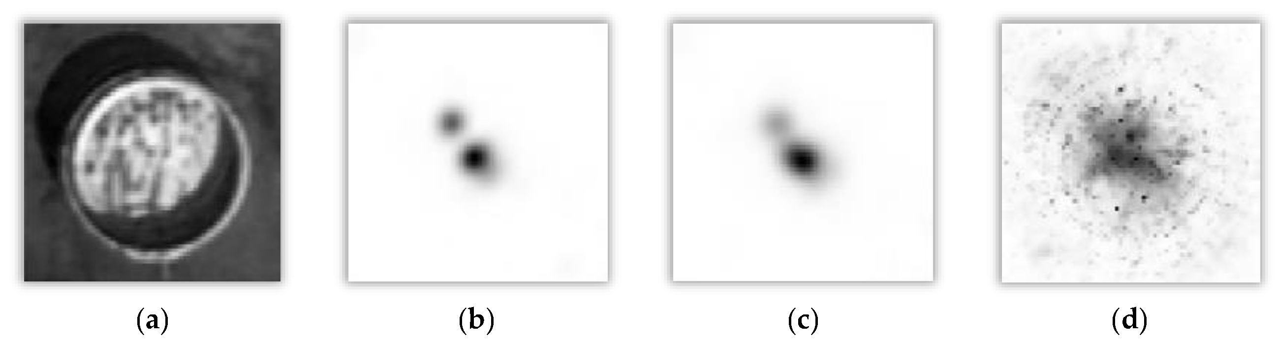
- When the floating roof of the oil tank is lower than the tank wall, there will be two areas that are brighter and darker in the image (as shown in Figure 7a), which makes positively affected pixels and negatively affected pixels at the boundary of the floating roof offset each other during transformation. Thus, the distribution of pixel values of orientation projection image and magnitude projection image is affected, and the final transformation result is affected. The solution to this problem in this study is to change the processing object of FRST from pixel to gradient modulus of pixel and cancel the positively affected pixel. Since the positively and negatively affected pixels play decisive roles in aggregating “black circle” (circle whose contour is darker than the background) and “white circle” (circle whose contour is brighter than the background), respectively, the coexistence of these two pixels makes FRST have the function of aggregating both “black circle” and “white circle” on an image. However, when the circle in the image is not a complete “black circle” or “white circle”, the coexistence of the positively and negatively affected pixels will interfere with each other, thus affecting the aggregation effect of circles. After all the pixels are processed into a gradient modulus, all circles in the image will become “white circles”, and then only negatively affected pixels need to be retained (because positively affected pixels have little effect on aggregating “white circles”), which solves the problem that some positively and negatively affected pixels offset each other during transformation.
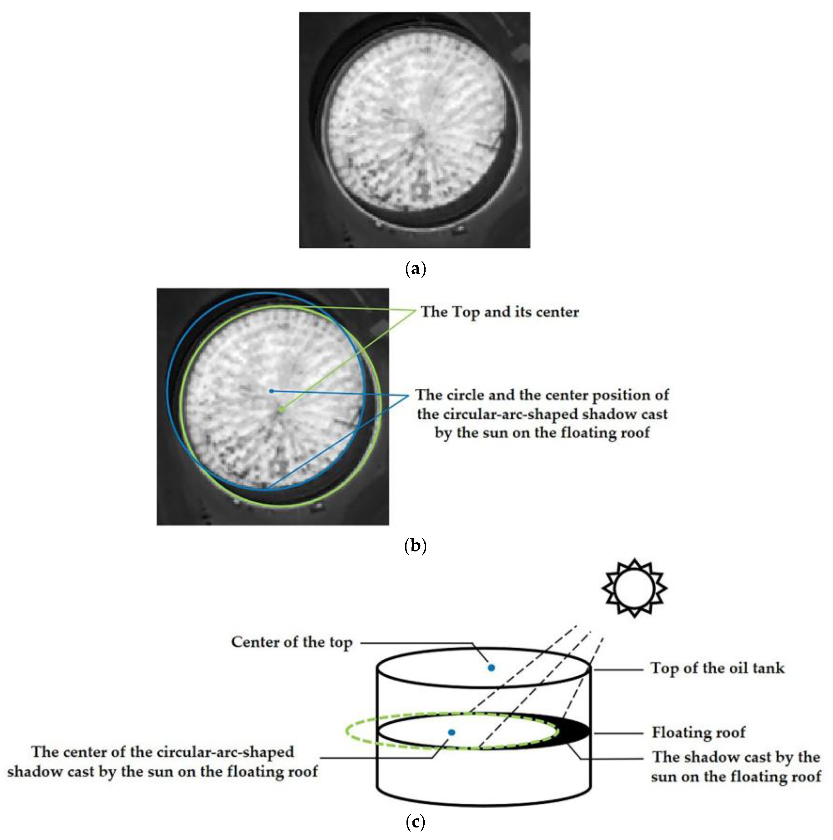
- In the transformation results, almost only one aggregation area can be seen (see Figure 7b,c), and it is impossible to distinguish the center of the tank roof from the center of the circular-arc-shaped shadow cast by the sun on the floating roof. Therefore, FRST cannot complete the accurate localization task of the oil tank in this study. In view of the fact that the positions of the two circle centers are close, and the blur effect of the 3 × 3 Sobel operator used in FRST to calculate the gradient will have an adverse effect on accurate localizing, a simple first-order difference is used to calculate the gradient instead in this study.
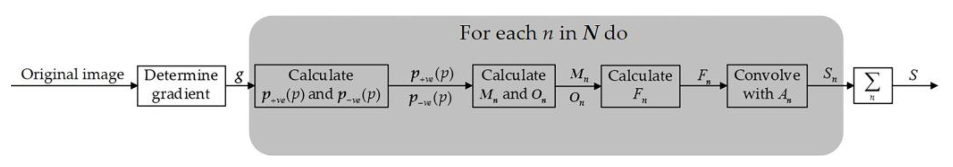
- The effect of the transformation is greatly limited by the range of the input radius, and the wider the range, the worse the effect, which leads to the transformation being extremely dependent on the priori knowledge of radius. It can be inferred that the parameters related to the radius in FRST are particularly important to the result. The value of scaling factor kn is 9.9 by default when the radius is not 1, but this value is an empirical value given in an experiment with a radius range of 2–30. However, in this study and practice, the radius may exceed 30. Therefore, in this study, Mn and On are normalized by dividing all pixels in Mn and On by the maximum value of pixels in Mn and On respectively instead of kn.
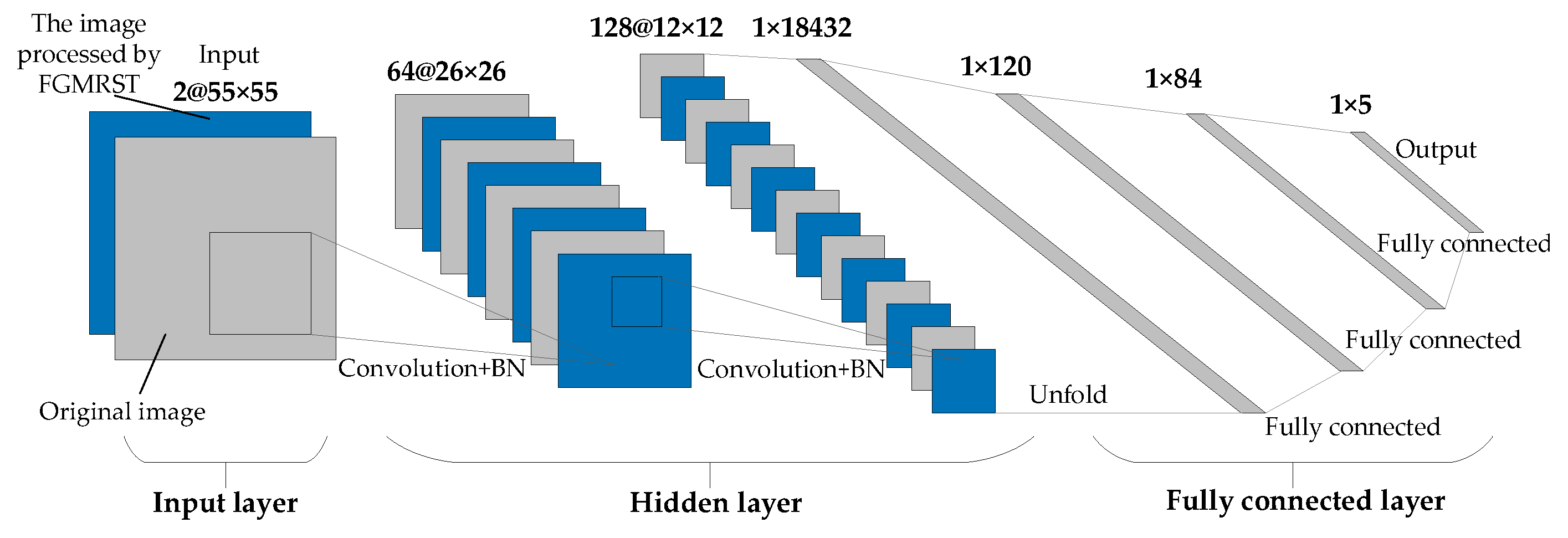
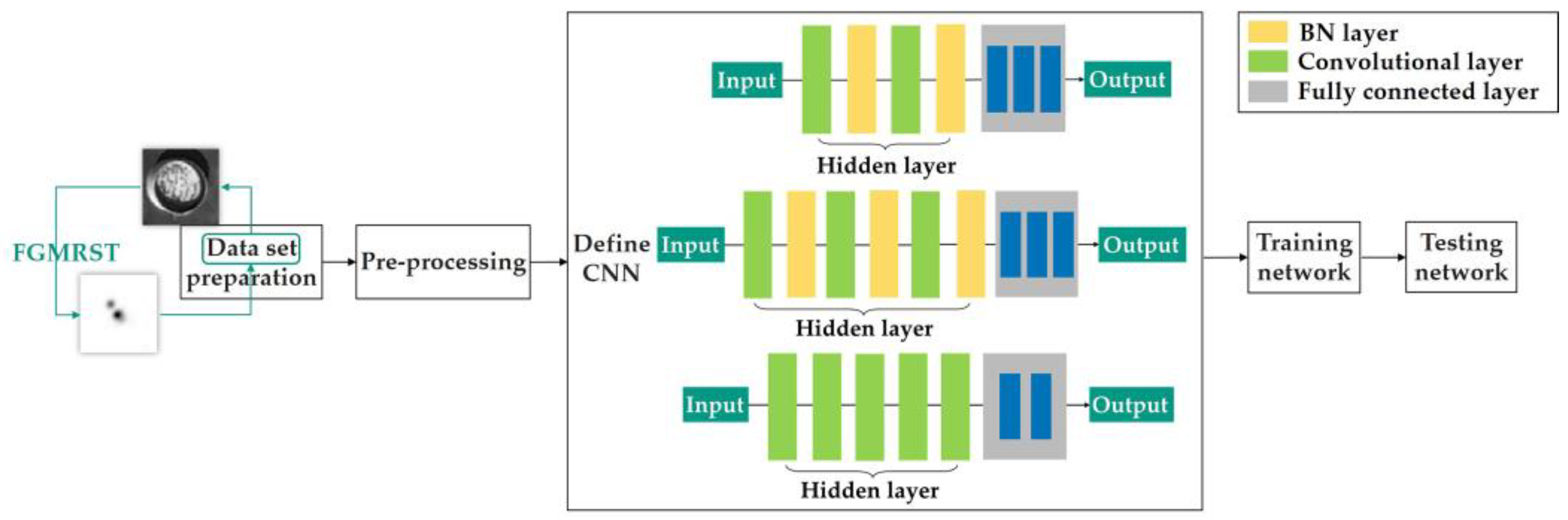
2.3. FGMRST-Based CNN Localization Method of the Oil Tank
2.3.1. Overview of Methods
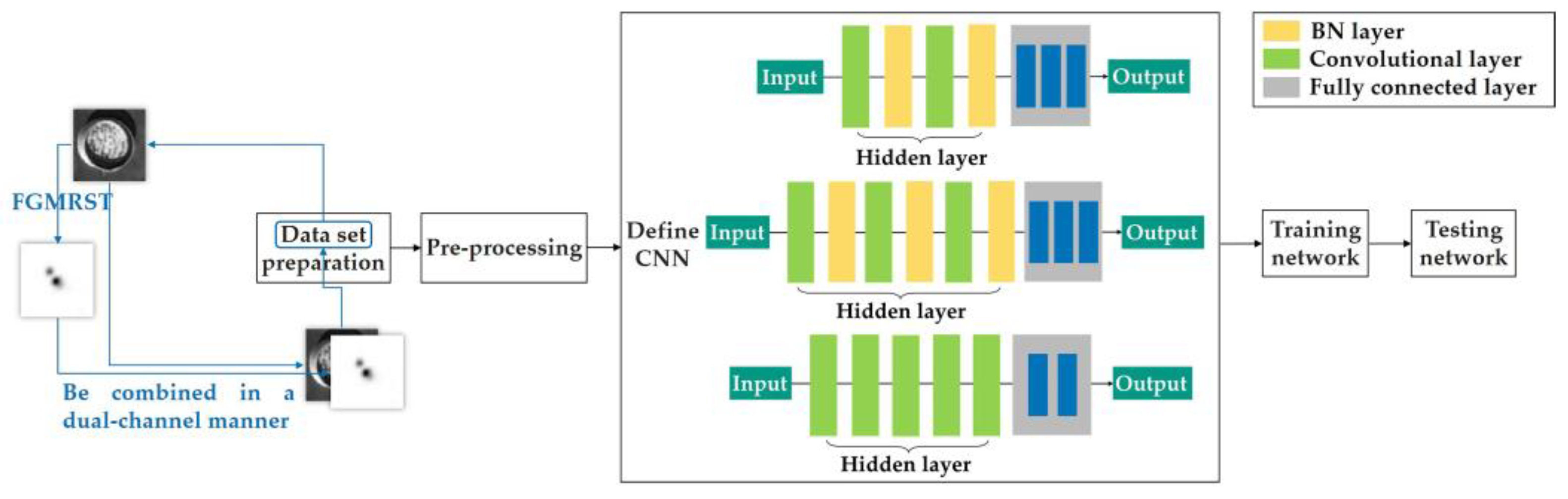
2.3.2. Flow of Methods
- 1.
- Data set preparation
- 2.
- Pre-processing
- 3.
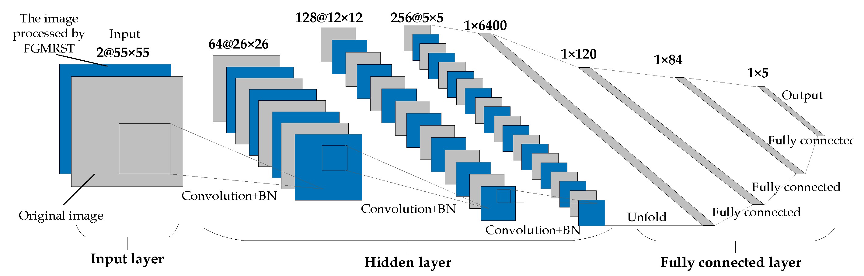
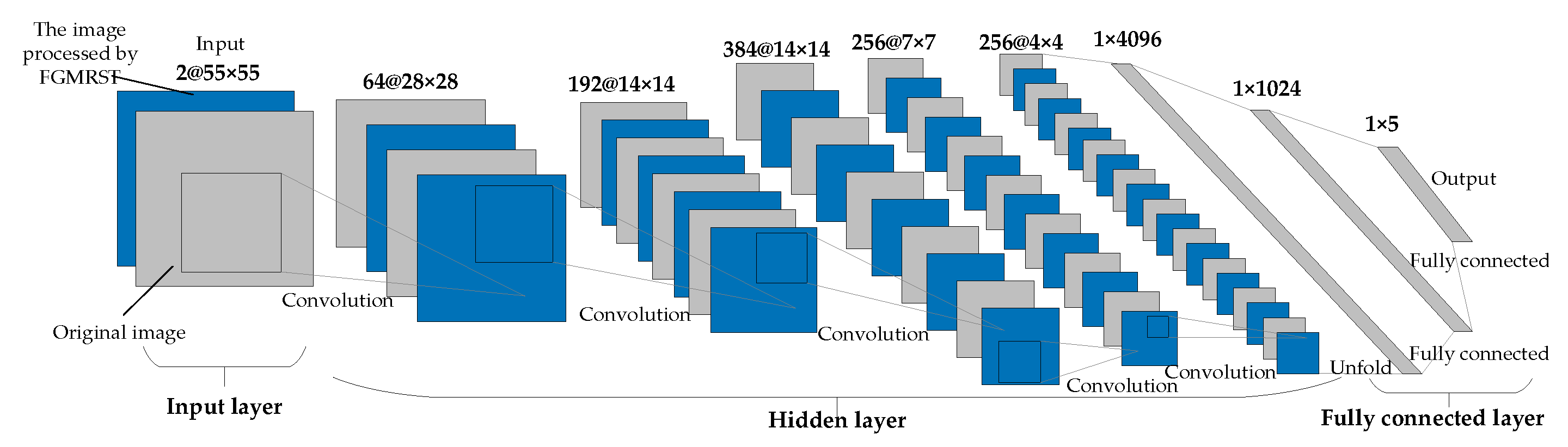
- Define CNN
- 4.
- Training network
- 5.
- Testing network on the test set
3. Experiments and Results
3.1. Training Details
3.2. Data sets
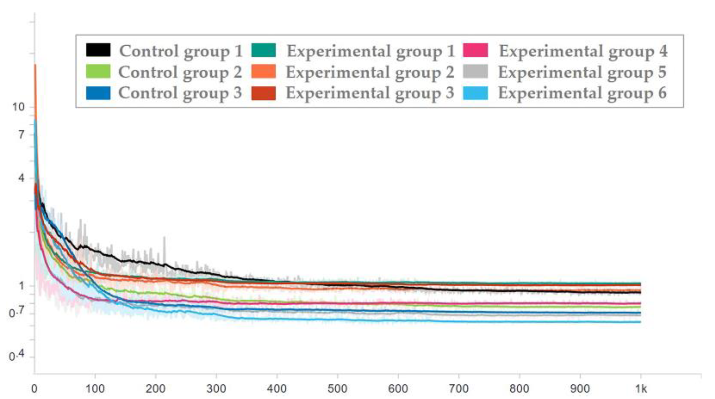
3.3. Experimental Process and Results
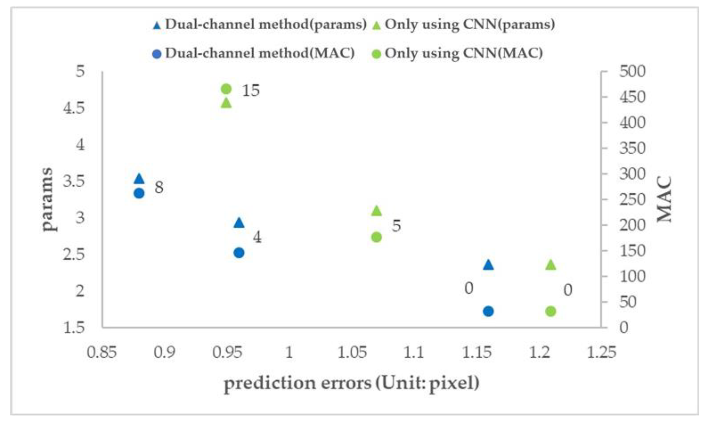
- When the number of additional convolution layers is 0, the number of parameters and computation (params and MAC) of the two methods are the same, but the prediction error of the dual-channel method is less than that of the ordinary CNN method.
- The prediction error of adding 4 layers in the dual-channel method is close to that of adding 15 layers in the ordinary CNN method, but the amount of parameters (params) of the latter is 1.6 times that of the former, and the amount of computation (MAC) of the latter is 3.2 times that of the former.
- The number of parameters and computation (params and MAC) of the two methods increases with the increase in the number of network layers, but the dual-channel method grows more slowly. Therefore, the dual-channel method effectively reduces the number of parameters and computation, that is, improves the computational efficiency.
4. Conclusions
- In the FGMRST-based CNN method, the average prediction error of the dual-channel method is reduced by 14.64% compared with the ordinary CNN method, which effectively improves the accuracy.
- In the shallowest network (net_conv2), the average prediction error of the dual-channel method is reduced by 19.66% compared with the ordinary CNN method. In the deeper network (net_conv3), the average prediction error is reduced by 15.73%. In the deepest network (net_alex), the average prediction error is reduced by 8.54%. It shows that the proposed method is still better than the method using only CNN when the number of network layers increases.
- In the FGMRST-based CNN method, the dual-channel method significantly improves the computational efficiency compared with the ordinary CNN method.
Author Contributions
Funding
Data Availability Statement
Conflicts of Interest
References
- Meng, F.S. Review of change detection methods based on Remote Sensing Images. Technol. Innov. Appl. 2012, 24, 57–58. [Google Scholar]
- Sui, X.L.; Zhang, T.; Qu, Q.X. Application of Deep Learning in Target Recognition and Position in Remote Sensing Images. Technol. Innov. Appl. 2019, 34, 180–181. [Google Scholar]
- Xu, H.P.; Chen, W.; Sun, B.; Chen, Y.F.; Li, C.S. Oil tank detection in synthetic aperture radar images based on quasi-circular shadow and highlighting arcs. J. Appl. Remote Sens. 2014, 8, 397–398. [Google Scholar] [CrossRef]
- Yu, S.T. Research on Oil Tank Volume Extraction Based on High Resolution Remote Sensing Image. Master’s Thesis, Dalian Maritime University, Liaoning, China, 2019. [Google Scholar]
- Ding, W. A Practical Measurement for Oil Tank Storage. J. Lanzhou Petrochem. Polytech. 2001, 1, 4–6. [Google Scholar]
- Duda, R.O.; Hart, P.E. Use of the Hough transformation to detect lines and curves in pictures. Commun. ACM 1972, 15, 11–15. [Google Scholar] [CrossRef]
- Shin, B.G.; Park, S.Y.; Lee, J.J. Fast and robust template matching algorithm in noisy image. In Proceedings of the International Conference on Control, Automation and Systems, Seoul, Korea, 17–20 October 2007. [Google Scholar]
- Wu, X.D.; Feng, W.F.; Feng, Q.Q.; Li, R.S.; Zhao, S. Oil Tank Extraction from Remote Sensing Images Based on Visual Attention Mechanism and Hough Transform. J. Inf. Eng. Univ. 2015, 16, 503–506. [Google Scholar]
- Han, X.W.; Fu, Y.L.; Li, G. Oil Depots Recognition Based on Improved Hough Transform and Graph Search. J. Electron. Inf. Technol. 2011, 33, 66–72. [Google Scholar] [CrossRef]
- Cai, X.Y.; Sui, H.G. A Saliency Map Segmentation Oil Tank Detection Method in Remote Sensing Image. Electron. Sci. Technol. 2015, 28, 154–156, 160. [Google Scholar]
- Zhang, W.S.; Wang, C.; Zhang, H.; Wu, F.; Tang, Y.X.; Mu, X.P. An Automatic Oil Tank Detection Algorithm Based on Remote Sensing Image. J. Astronaut. 2006, 27, 1298–1301. [Google Scholar]
- Hinton, G.; Osindero, S.; Teh, Y. A Fast Learning Algorithm for Deep Belief nets. Neural. Comput. 2006, 18, 1527–1554. [Google Scholar] [CrossRef] [PubMed]
- Lecun, Y.; Bengio, Y.; Hinton, G. Deep learning. Nature 2015, 521, 436. [Google Scholar] [CrossRef] [PubMed]
- Sun, Z.J.; Xue, L.; Xu, Y.M. Overview of deep learning. Appl. Res. Comput. 2012, 29, 2806–2810. [Google Scholar]
- Lecun, Y.; Boser, B.; Denker, J.S.; Henderson, D.; Howard, R.; Hubbard, W.; Jackel, L. Backpropagation Applied to Handwritten Zip Code Recognition. Neural. Comput. 1989, 1, 541–551. [Google Scholar] [CrossRef]
- Krizhevsky, A.; Sutskever, I.; Hinton, G. ImageNet Classification with Deep Convolutional Neural Networks. In Proceedings of the Annual Conference on Neural Information Processing Systems, Lake Tahoe, NV, USA, 3–8 December 2012. [Google Scholar]
- Deep Residual Learning for Image Recognition. Available online: https://arxiv.org/pdf/1512.03385.pdf (accessed on 1 October 2020).
- Wang, Y.J.; Zhang, Q.; Zhang, Y.M.; Meng, Y.; Guo, W. Oil Tank Detection from Remote Sensing Images based on Deep Convolutional Neural Network. Remote Sens. Technol. Appl. 2019, 34, 727–735. [Google Scholar]
- Loy, G.; Zelinsky, A. Fast radial symmetry for detecting points of interest. IEEE Trans. Pattern Anal. Mach. Intell 2003, 25, 959–973. [Google Scholar] [CrossRef] [Green Version]
- Gong, R. Sky Sat. Satell. Appl. 2016, 7, 82. [Google Scholar]
- Reisfeld, D.; Wolfson, H.; Yeshurun, Y. Context-free attentional operators: The generalized symmetry transform. Int. J. Comput. Vis. 1995, 14, 119–130. [Google Scholar] [CrossRef]
- Intrator, N.; Reisfeld, D.; Yeshurun, Y. Extraction of Facial Features for Recognition using Neural Networks. Acta Obs. Gynecol Scand. 1995, 19, 1–167. [Google Scholar]
- Reisfeld, D.; Yeshurun, Y. Preprocessing of Face Images: Detection of Features and Pose Normalization. Comput. Vis. Image Underst. 1998, 71, 413–430. [Google Scholar] [CrossRef]
- Sela, G.; Levine, M.D. Real-Time Attention for Robotic Vision. Real-Time Imaging 1997, 3, 173–194. [Google Scholar] [CrossRef] [Green Version]
- Kimme, C.; Balard, D.; Sklansky, J. Finding Circles by an Array of Accumulators. Commun. ACM 1975, 18, 120–122. [Google Scholar] [CrossRef]
- Minor, L.G.; Sklansky, J. The Detection and Segmentation of Blobs in Infrared Images. IEEE Trans. Syst. Man Cybern. 1981, 11, 194–201. [Google Scholar] [CrossRef]
- Ok, A.O.; Baseski, E. Circular Oil Tank Detection from Panchromatic Satellite Images: A New Automated Approach. IEEE Geosci. Remote Sens. Lett. 2015, 12, 1347–1351. [Google Scholar] [CrossRef]
- Khan, S.H.; Bennamoun, M.; Sohel, F.; Togneri, R. Automatic Shadow Detection and Removal from a Single Image. IEEE Trans. Pattern Anal. Mach. Intell 2016, 38, 431–446. [Google Scholar] [CrossRef] [PubMed] [Green Version]
- Guo, R.Q.; Dai, Q.Y.; Hoiem, D. Paired Regions for Shadow Detection and Removal. IEEE Trans. Pattern Anal. Mach. Intell 2013, 35, 2956–2967. [Google Scholar] [CrossRef] [PubMed]
- Guo, R.Q.; Dai, Q.Y.; Hoiem, D. Single-image shadow detection and removal using paired regions. In Proceedings of the IEEE Conference on Computer Vision and Pattern Recognition, Colorado Springs, CO, USA, 20–25 June 2011. [Google Scholar]


| Calculation Location | Whether the Features at the Circumference Can Be Processed | ||
|---|---|---|---|
| Convolution | FGMRST | Convolution + FGMRST | |
| Circumference | √ | × | √ |
| Circle center | × | √ | √ |
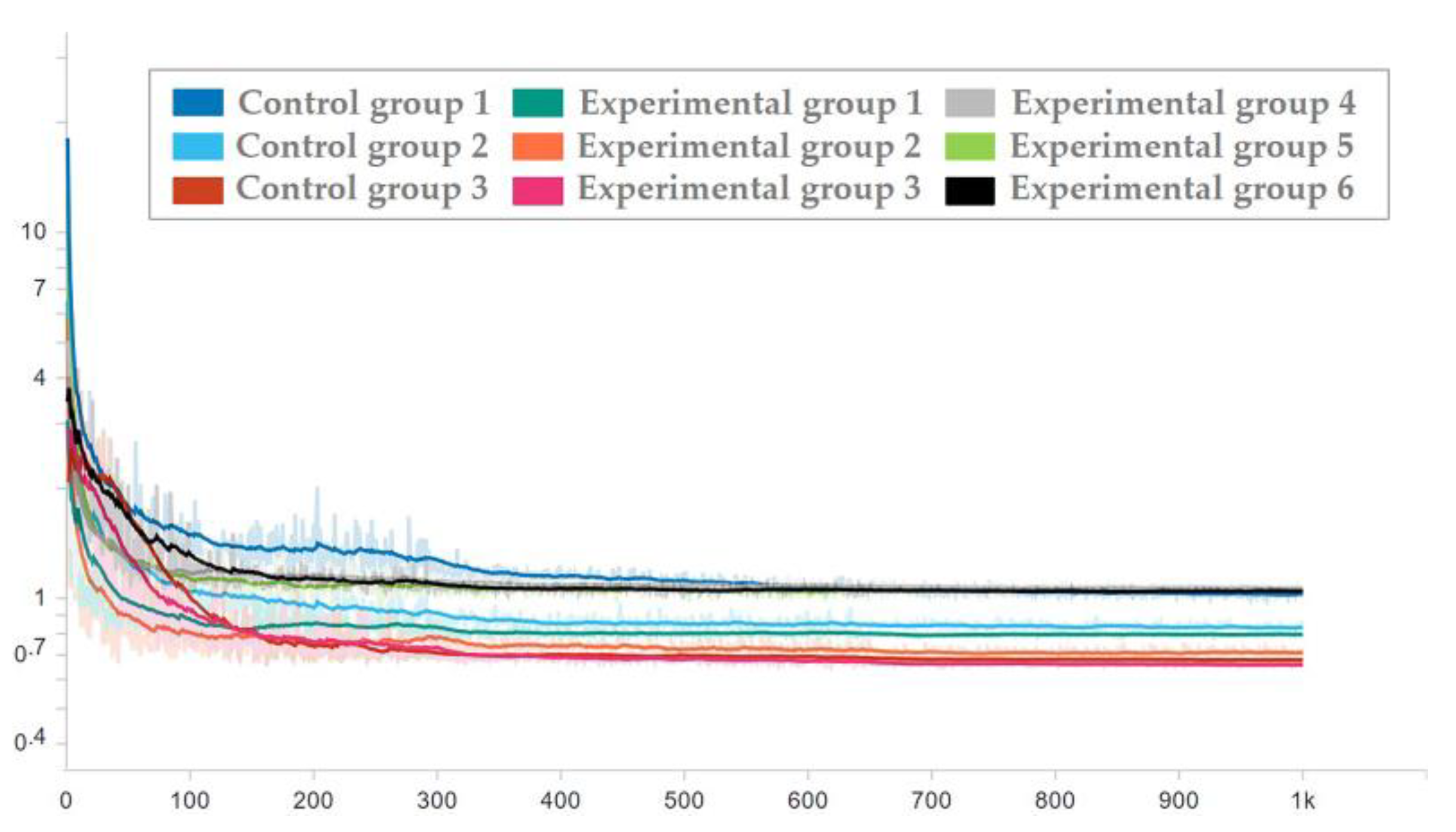
| Experimental Types | Way | Network Structures |
|---|---|---|
| Control group 1: original image→shallow CNN | Only using CNN | net_conv2 |
| Control group 2: original image→deeper CNN | net_conv3 | |
| Control group 3: original image→modified AlexNet | net_alex | |
| Experimental group 1: FGMRST→shallow CNN | Tandem method | net_conv2 |
| Experimental group 2: FGMRST→deeper CNN | net_conv3 | |
| Experimental group 3: FGMRST→modified AlexNet | net_alex | |
| Experimental group 4: original image + FGMRST→shallow CNN | Dual-channel method | net_conv2 |
| Experimental group 5: original image + FGMRST→deeper CNN | net_conv3 | |
| Experimental group 6: original image + FGMRST→modified AlexNet | net_alex |
| Random Seed | Experimental Types | Way | Network Structures | Learning Rate | Average Prediction Errors (Unit: Pixel) |
|---|---|---|---|---|---|
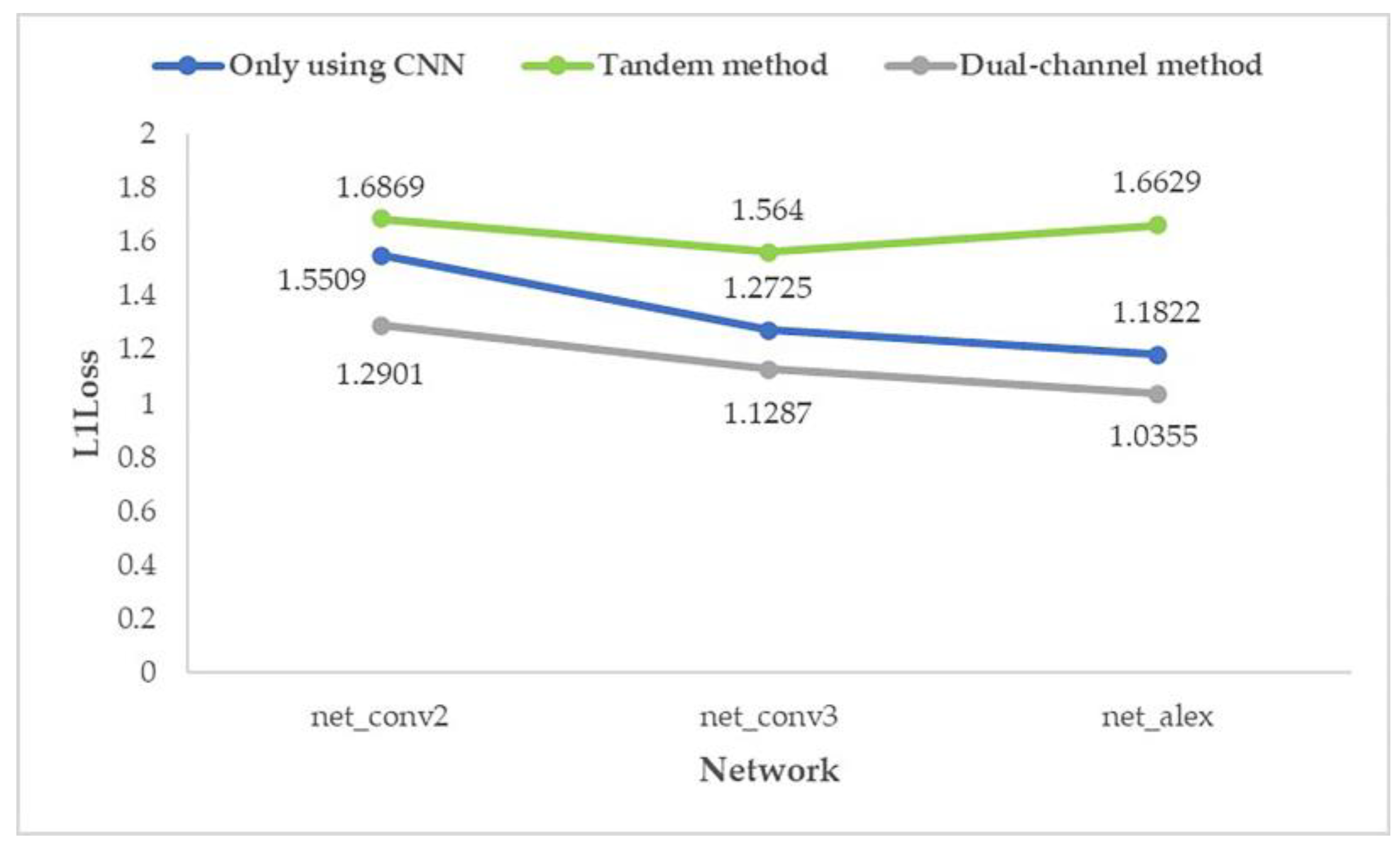
| 0 | Control group 1 | Only using CNN | net_conv2 | 0.0025 | 1.5509 |
| Control group 2 | net_conv3 | 0.0025 | 1.2725 | ||
| Control group 3 | net_alex | 0.00125 | 1.1822 | ||
| Experimental group 1 | Tandem method | net_conv2 | 0.00125 | 1.6869 | |
| Experimental group 2 | net_conv3 | 0.00125 | 1.5640 | ||
| Experimental group 3 | net_alex | 0.00125 | 1.6629 | ||
| Experimental group 4 | Dual-channel method | net_conv2 | 0.0025 | 1.2901 | |
| Experimental group 5 | net_conv3 | 0.0025 | 1.1287 | ||
| Experimental group 6 | net_alex | 0.00125 | 1.0355 1 | ||
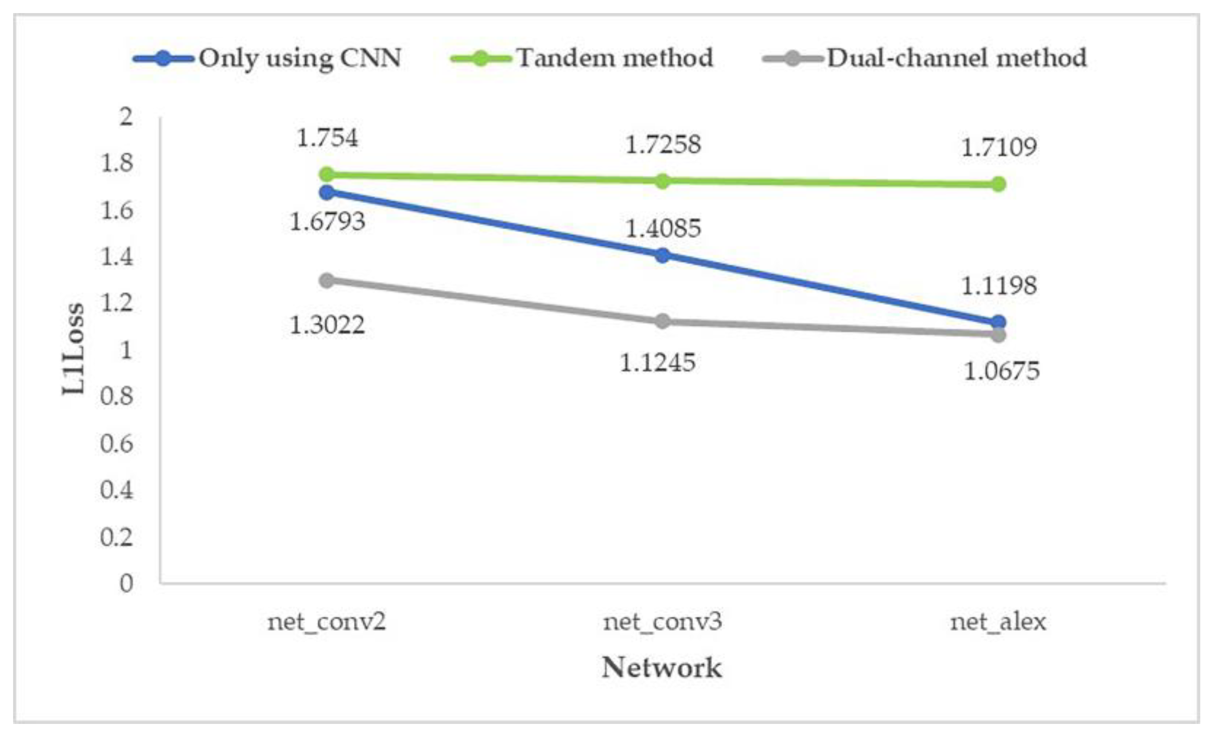
| 1 | Control group 1 | Only using CNN | net_conv2 | 0.0025 | 1.6793 |
| Control group 2 | net_conv3 | 0.0025 | 1.4085 | ||
| Control group 3 | net_alex | 0.00125 | 1.1198 | ||
| Experimental group 1 | Tandem method | net_conv2 | 0.00125 | 1.7540 | |
| Experimental group 2 | net_conv3 | 0.00125 | 1.7258 | ||
| Experimental group 3 | net_alex | 0.00125 | 1.7109 | ||
| Experimental group 4 | Dual-channel method | net_conv2 | 0.0025 | 1.3022 | |
| Experimental group 5 | net_conv3 | 0.0025 | 1.1245 | ||
| Experimental group 6 | net_alex | 0.00125 | 1.0675 |
| Way | Parameter | Additional Convolution Layers Added on net_conv3 | ||
|---|---|---|---|---|
| 0 | 5 | 15 | ||
| Only using CNN | Params(e+00M) | 2.357 | 3.095 | 4.571 |
| MAC(e+00M) | 30.42 | 174.9 | 463.9 | |
| Prediction errors (Unit: pixel) | 1.21 | 1.07 | 0.95 | |
| Way | Parameter | Additional Convolution Layers Added on net_conv3 | ||
| 0 | 4 | 8 | ||
| Dual-channel method | Params(e+00M) | 2.357 | 2.933 | 3.527 |
| MAC(e+00M) | 30.42 | 145.1 | 260.8 | |
| Prediction errors (Unit: pixel) | 1.16 | 0.96 | 0.88 | |
Publisher’s Note: MDPI stays neutral with regard to jurisdictional claims in published maps and institutional affiliations. |
© 2021 by the authors. Licensee MDPI, Basel, Switzerland. This article is an open access article distributed under the terms and conditions of the Creative Commons Attribution (CC BY) license (https://creativecommons.org/licenses/by/4.0/).
Share and Cite
Jiang, H.; Zhang, Y.; Guo, J.; Li, F.; Hu, Y.; Lei, B.; Ding, C. Accurate Localization of Oil Tanks in Remote Sensing Images via FGMRST-Based CNN. Remote Sens. 2021, 13, 4646. https://doi.org/10.3390/rs13224646
Jiang H, Zhang Y, Guo J, Li F, Hu Y, Lei B, Ding C. Accurate Localization of Oil Tanks in Remote Sensing Images via FGMRST-Based CNN. Remote Sensing. 2021; 13(22):4646. https://doi.org/10.3390/rs13224646
Chicago/Turabian StyleJiang, Han, Yueting Zhang, Jiayi Guo, Fangfang Li, Yuxin Hu, Bin Lei, and Chibiao Ding. 2021. "Accurate Localization of Oil Tanks in Remote Sensing Images via FGMRST-Based CNN" Remote Sensing 13, no. 22: 4646. https://doi.org/10.3390/rs13224646
APA StyleJiang, H., Zhang, Y., Guo, J., Li, F., Hu, Y., Lei, B., & Ding, C. (2021). Accurate Localization of Oil Tanks in Remote Sensing Images via FGMRST-Based CNN. Remote Sensing, 13(22), 4646. https://doi.org/10.3390/rs13224646