Article

Knowledge Distillation of Grassmann Manifold Network for Remote Sensing Scene Classification

1
Electronic Information School, Wuhan University, Wuhan 430072, China
2
School of Computer Science, Wuhan University, Wuhan 430072, China
*
Author to whom correspondence should be addressed.
Remote Sens. 2021, 13(22), 4537; https://doi.org/10.3390/rs13224537
Submission received: 8 September 2021 / Revised: 23 October 2021 / Accepted: 8 November 2021 / Published: 11 November 2021

Abstract

:
Due to device limitations, small networks are necessary for some real-world scenarios, such as satellites and micro-robots. Therefore, the development of a network with both good performance and small size is an important area of research. Deep networks can learn well from large amounts of data, while manifold networks have outstanding feature representation at small sizes. In this paper, we propose an approach that exploits the advantages of deep networks and shallow Grassmannian manifold networks. Inspired by knowledge distillation, we use the information learned from convolutional neural networks to guide the training of the manifold networks. Our approach leads to a reduction in model size, which addresses the problem of deploying deep learning on resource-limited embedded devices. Finally, a series of experiments were conducted on four remote sensing scene classification datasets. The method in this paper improved the classification accuracy by 2.31% and 1.73% on the UC Merced Land Use and SIRIWHU datasets, respectively, and the experimental results demonstrate the effectiveness of our approach.

Graphical Abstract

1. Introduction

In recent years, high-resolution remote sensing (HRRS) images have become more accessible with the development of satellite and remote sensing technologies, which provide detailed information on the land surface. Therefore, many remote sensing image tasks are also developing rapidly, such as semantic segmentation [1,2], object detection [3] and scene classification. Remote sensing image semantic segmentation has been widely used in various applications, such as natural resource protection, change detection [4] and other applications [5,6]. Objects in high-resolution remote sensing images have rich details, such as geometry and structure, which bring more challenges to land use classification. The scene classification of optical remote sensing images can be divided into two categories, namely, methods based on artificially designed features and methods based on deep features. The hand-crafted features used for optical remote sensing image scene classification can be broadly classified into three categories, namely, spectral features, texture features, and structural features. Commonly used spectral features include image gray value, gray value mean, and gray value variance. Literature [7] directly uses image gray value as a classification feature, while literature [8,9] takes gray mean and variance as classification features. Local Binary Pattern (LBP) and Gray Level Co-occurrence Matrix (GLCM) are typical texture features. Scale-invariant feature transform (SIFT) is an effective structural feature [8,9,10], in addition to the line segment [11], wavelet transform [9] and Gabor transform [12]. However, the methods of hand-crafted features have the limitations of poor data adaptability and low feature utilization. The effectiveness of deep learning in remote sensing images has recently received a lot of attention. Methods based on fusing deep features [13,14,15] increase the information content of the features by fusing one or more CNN features from different layers and improve the classification performance. Cheng et al. [14] proposed the bag of convolutional features for optical remote sensing image scene classification based on the idea of the BoVW model. Xu et al. [16] proposed a GLDBS model to learn global and local information from the original image and the key location. A two-stream feature aggregation deep neural network (TFADNN) [17] was developed to obtain reasonable descriptions of HSR images, which contains the stream of discriminative features and the stream of general features. Xu et al. [18] developed a deep feature aggregation framework driven by graph convolutional network (DFAGCN), and it employs a pretrained CNN to obtain multilayer features and utilizes a graph convolutional network-based model to reveal patch-to-patch correlations between the feature maps. Bi et al. [19] presented a local semantic enhanced ConvNet(LSE-Net) and a context-aware class peak response(CACPR) measurement to mimic the top-down human vision perception. Li et al. [20] designed a discriminative learning of adaptive match network (DLA-MatchNet) for few-shot remote sensing scene images, and it employs the channel attention and spatial attention modules to learn discriminative feature representation. Deng et al. [21] propoed a joint network combined CNNs and vision transformer(CTNet), and a joint loss function is designed to optimize the network.
The framework of the deep network can be divided into three parts: feature extraction module, quantization module, and optimization strategy. The quantization module mainly includes spatial quantization, amplitude quantization, and evaluation quantization. A typical spatial quantization is pooling, which can reduce the number of parameters and mitigate the impact of overfitting problems. Some activation functions, such as sigmoid and ReLU [22], are examples of amplitude quantization. It maps real values to a specific range in a nonlinear manner. Evaluation quantization is used to output data in a desirable form, such as softmax. A large number of optimization strategies, such as stochastic gradient descent (SGD) and Adam [
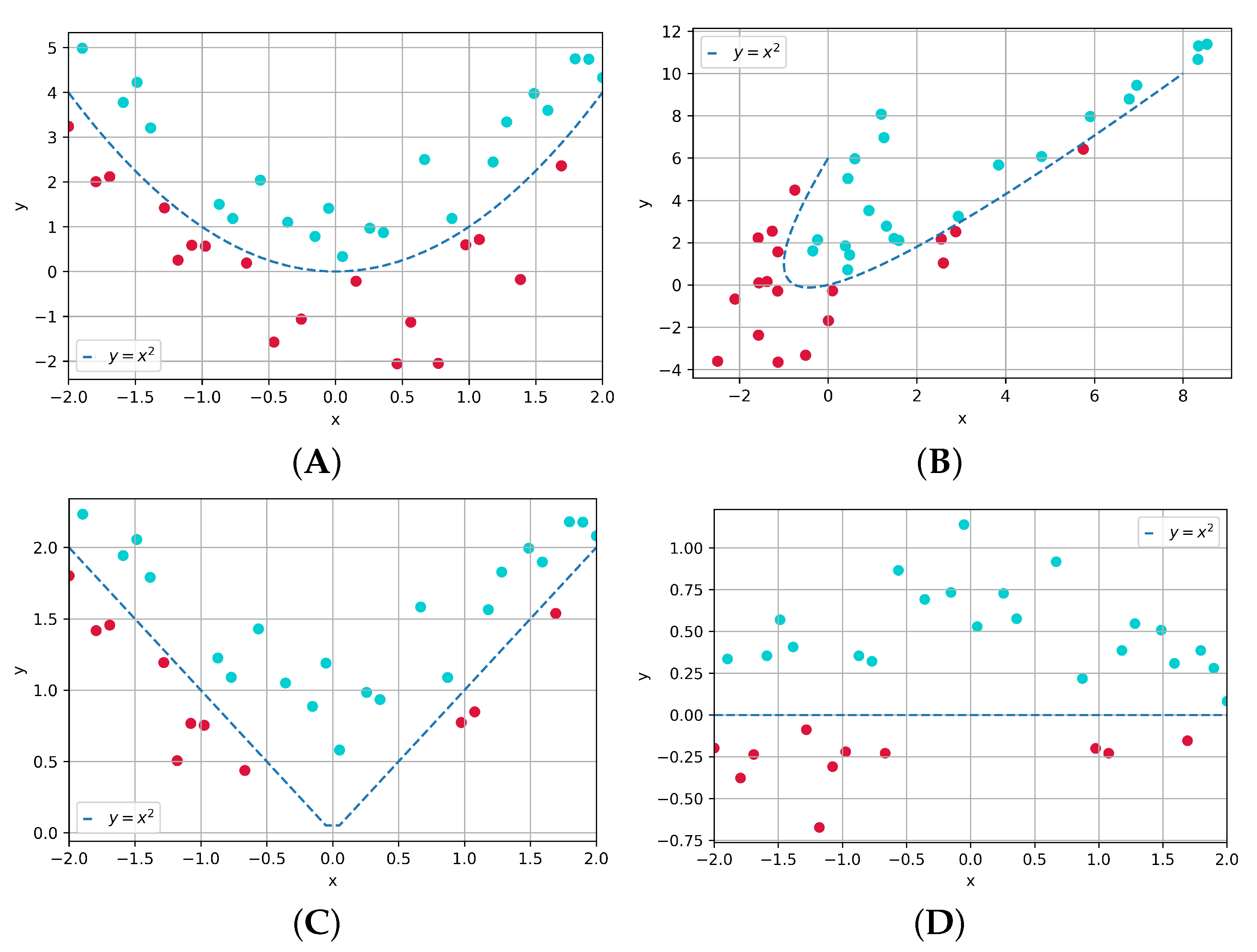
23], have been proposed to speed up network convergence and improve the stability of training. Convolutional neural networks greatly reduce the number of parameters by sharing convolutional kernels, and multiple convolutional kernels can extract different types of features. The convolution kernel slides over the feature map and performs cross-correlation operations with the corresponding regions on the feature map, so the convolution is linear. We can discuss neural networks and classification from the perspective of spatial transformations. Classification can be seen as performing certain spatial transformations on the data, changing the distribution of the data so that eventually a hyperplane can be found to separate the different classes of data. However, the data characterization capability of a linear transformation is limited. Subfigure A in Figure 1 shows the original data distribution, the second subfigure shows the distribution of the data after linear transformation, the subfigure C and subfigure D are the distribution of the data after nonlinear transformation. It’s obvious that the nonlinear transformation makes the data more separable. Therefore, it is necessary to add an activation function after the convolution layer, which acts as a nonlinear transform. A simple and effective activation function is the Rectified Linear Unit (ReLU). To make the data more separable, it is necessary to deepen the network to enhance its transformation capabilities. The pooling layer reduces the dimensionality of the representation and prevents overfitting. The fully connected layer can map the feature space to the label space, where some evaluation quantization is utilized to achieve better classification.
A manifold is a general term for geometric objects, including curves and surfaces of various dimensions. According to the manifold hypothesis, data in high-dimensional space exist on or near a low-dimensional manifold, which determines the invariance of the data, and the coordinates on the manifold correspond to the core variables of the data. From the perspective of manifold, the classification algorithm aims to separate a bunch of manifolds. The purpose of manifold learning is to determine the internal mapping between the original high-dimensional data and the actual low-dimensional manifold structure. As long as we can learn the manifolds correctly, we can accomplish a complete knowledge of the data and thus derive the nature of the whole data from the partial sample rules. Thus, manifold learning can be seen as a method of dimensionality reduction. Traditional manifold learning can be divided into global learning methods and local learning methods. Global manifold methods consider the structural relationships between all data pairs as equally important for the determination of manifold embeddings and attempt to maintain the global structure of the original space in the low-dimensional manifold space. Typical global methods include multidimensional scaling (MDS) [24] and Isometric feature mapping (ISOMAP) [25]. The local manifold method considers that the key to manifold embedding is the structure information of the local region, so the focus of manifold learning is on the accurate modeling of the local structure, which reduces the computational effort to some extent. Locally linear embedding (LLE) [26] is a typical local method. It assumes that a manifold can be considered as a linear Euclidean space in its local neighborhood, and the local geometric description of the original data space is also valid in the low-dimensional manifold space. Other local methods include Laplacian eigenmaps (LE) [27]. Manifold learning is a nonlinear transformation, so it has a natural superiority over convolution in space transformation.
Convolutional neural networks cannot handle input data samples that reside on Riemannian manifolds, such as the manifolds of symmetric positive definite (SPD) matrices and the Grassmannian, so some work has focused on deep neural networks with points on the manifold as input. In [28], the authors propose a two-layer deep manifold network called GrNet, containing three innovative blocks. The input data of GrNet are points located on the Grassmann manifolds. In [29], a deep network architecture for input data residing on the manifold of symmetric positive definite matrices is introduced. In [30] the weighted Fréchet mean (wFM) [31] is used as an analog of convolution operation of manifold-valued data. However, the convexity constraint for wFM limits the value range of wFM, resulting in the limitation of the generalization ability of the model.
Although convolutional neural networks and deep manifold networks are both data-based, there are differences between them. In addition to the input data format, the size of the network also varies greatly. The convolution is a linear transformation, which leads to a relatively weak data characterization ability. Therefore, convolutional neural networks are stacked by many layers to achieve better performance. However, the computation of curved manifolds lies in non-Euclidean space, which has a more powerful characterization than convolution due to its nonlinearity. Consequently, manifold networks can have relatively excellent performance with fewer layers than convolutional neural networks.
In some practical scenarios, such as satellites, drones, and micro-robots, huge deep networks are not feasible. A smaller model has a smaller number of parameters but inevitably leads to a decrease in accuracy. Common approaches to model compression include pruning, quantization, hand-designed networks, and knowledge distillation. Manifold networks are small in size and can be used for the deployment of resource-limited devices. However, its generalization ability is not as good as large convolutional neural networks. Therefore, we propose to transfer the knowledge learned from convolutional neural networks to manifold networks using knowledge distillation. Most of the existing knowledge distillation methods are used between convolutional neural networks and thus will fail to overcome the drawbacks of convolution. On the other hand, current manifold networks are not mature enough to stack many layers like convolutional neural networks, so there is still a performance gap compared with convolutional neural networks. The CNNs can learn knowledge from large amounts of data, while the curve manifold learning has a better characterization of the nature of the data. Therefore, we expect to combine the advantages of deep learning and manifold learning through knowledge distillation.
To the above problems, this paper proposes a knowledge distillation-based method to train the Grassmann manifold network for remote sensing scene classification. The deep convolutional neural networks are used to guide the training process of shallow manifold networks, thus enabling the small manifold networks to acquire knowledge learned from large amounts of data. In the meantime, the size of the final network is small due to the effective characterization of the curve manifold.
Our contributions in this paper are as follows:
1
Through knowledge distillation, deep convolutional neural networks are allowed to train shallow manifold networks to seek better classification mappings at a smaller network size. In this way, the shallow manifold network learns information from a large amount of data while maintaining its excellent data characterization capability.
2
We first realize the flow and transmission of information between the manifold network and convolutional neural network. Since the input data of the two networks are located in different spaces, convolutional neural networks and manifold networks are inherently incompatible. For the first time, we have broken down the isolation between them, enabling the flow of information between the two networks and providing direction for communication between the other networks.
3
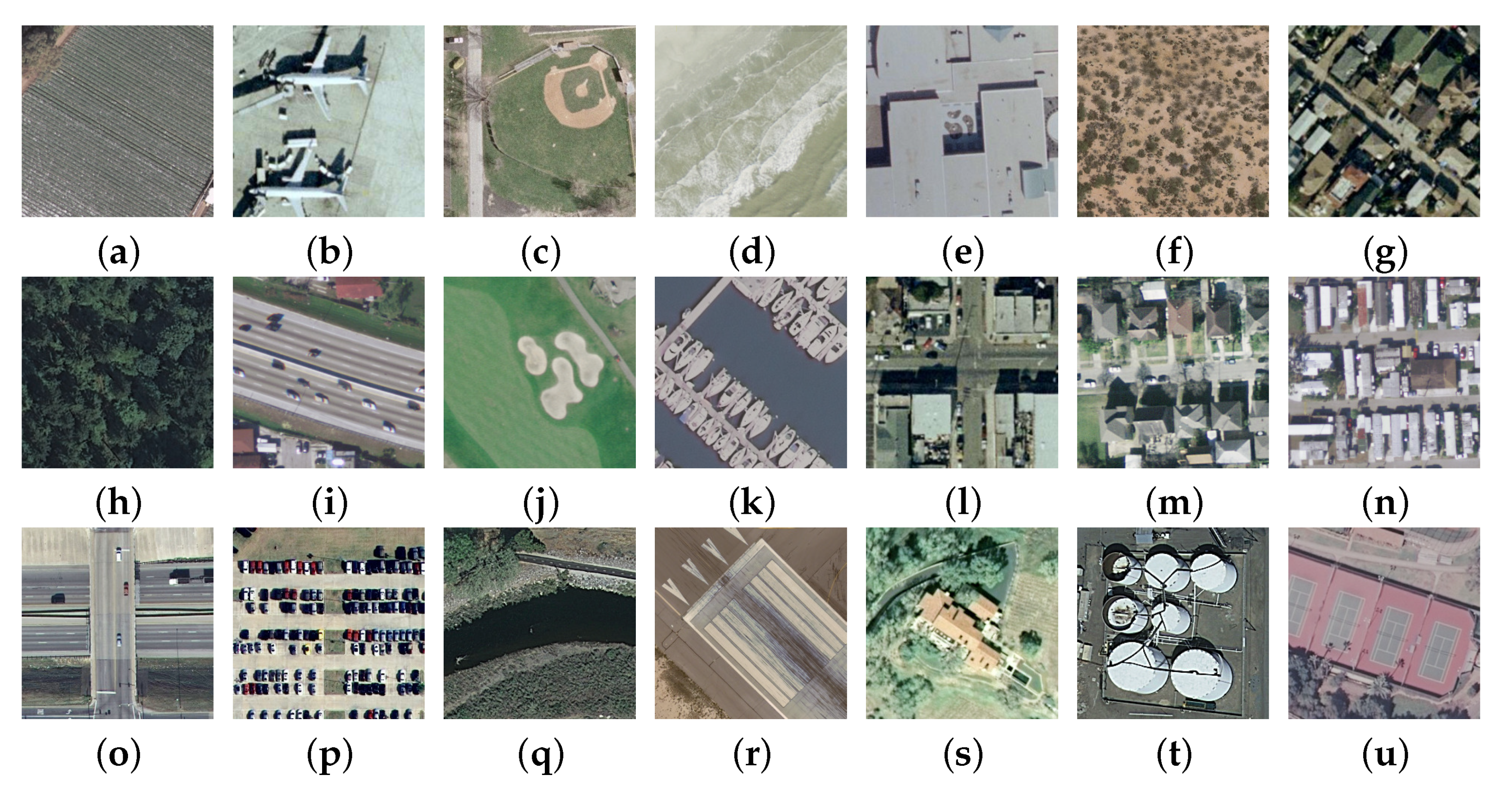
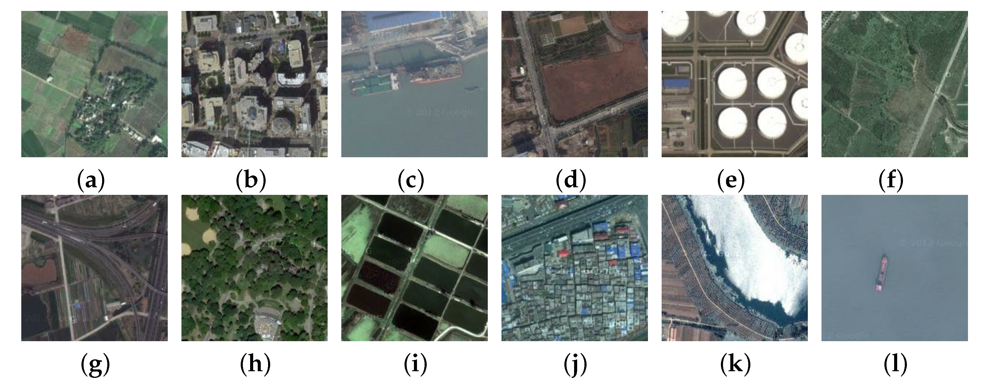
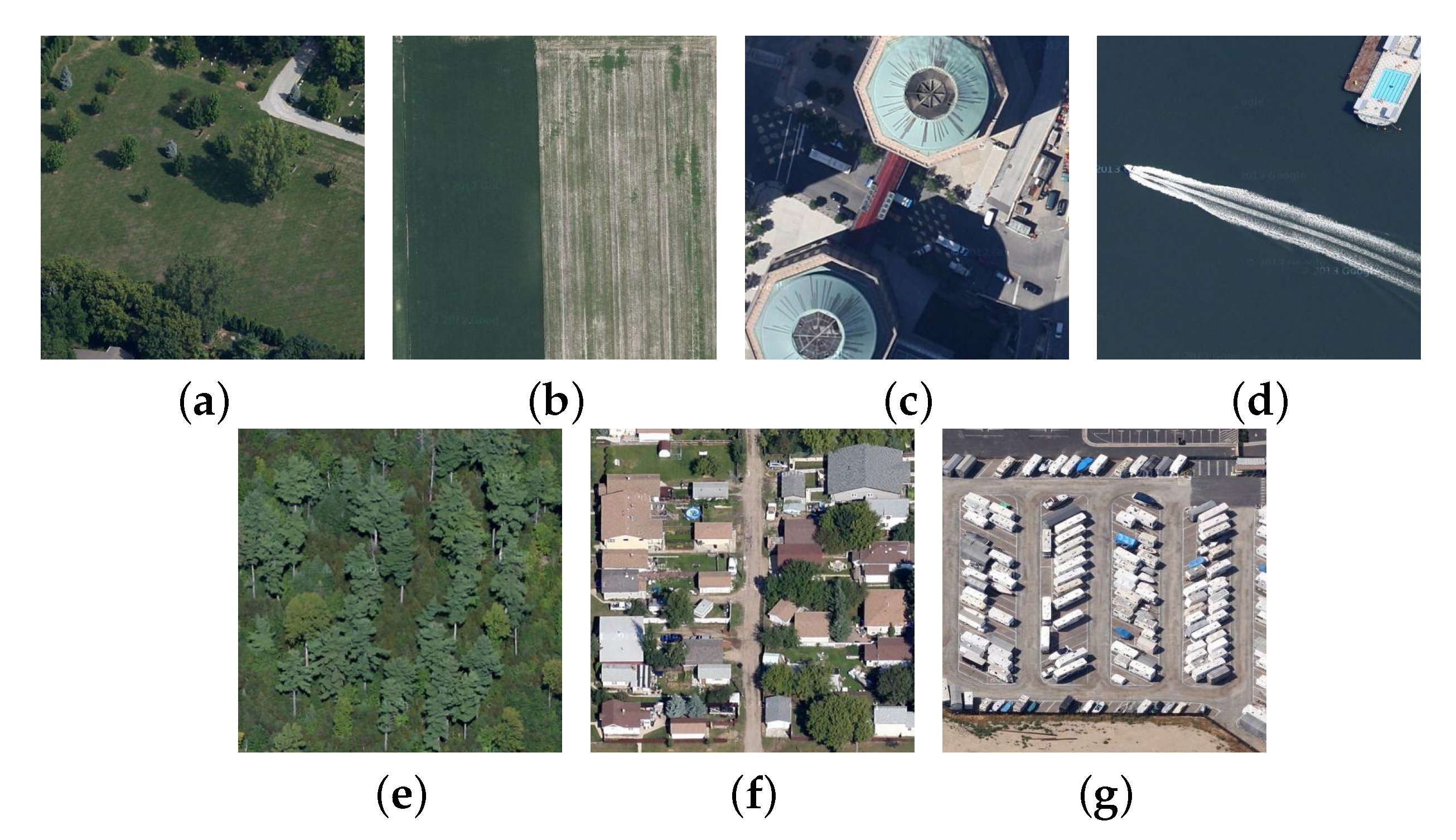
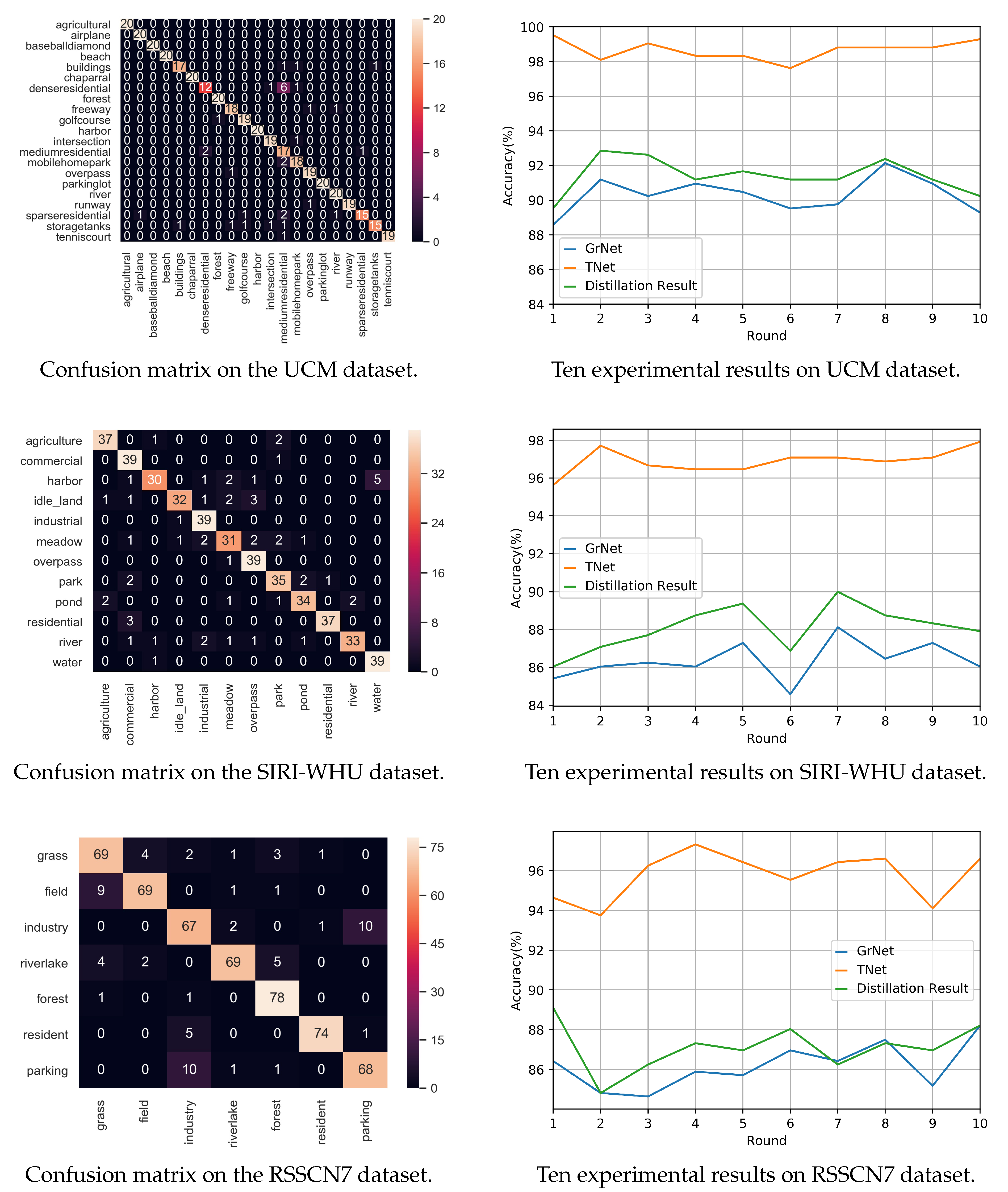
Experiments are carried out on three common standard datasets, namely UC Merced Land Use, SIRI-WHU, and RSSCN7 datasets. The accuracy of each dataset can be effectively improved, and the effectiveness of our method is verified.
The content of this paper is arranged as follows: Section 2 begins with a brief review of Grassmann networks and knowledge distillation, followed by a detailed description of our methodology. The experimental results and analysis are described in Section 3. In Section 4, we discuss the experimental results and the influence of the parameters on the experiment. Finally, the conclusion of this paper is given in Section 5.

2. Materials and Methods

In this section, a brief introduction to Grassman Network (GrNet) and knowledge distillation is given first. Then we will describe the proposed method in detail.

2.1. Grassmann Network (GrNet)

GrNet [28] is a Grassmann manifold network. The input of GrNet is Grassmannian data, which lies on the Grassmann manifold. A Grassmann manifold G r ( q , n ) is a compact Riemannian manifold, which is the set of all q-dimensional linear subspaces of R n that can be spanned by an orthonormal basis matrix X R n × q . Therefore we have:
G r ( q , n ) = { X R n × q X T X = I q }
where I q is the identity matrix of size q × q . The operations in Euclidean space are no longer feasible in Non-Euclidean space, so Riemannian calculations [32] and matrix backpropagation [33] on Grassmannian data are adopted to train the manifold network.
Features are extracted from successive frames of the face video and then processed so that they form a linear subspace [34,35], which is the Grassmannian manifold data. The Projection block consists of full rank mapping (FRMap) layers and re-orthonormalization (ReOrth) layers, which transform the input Grassmannian manifold data into a more discriminative and compact Grassmannian representation for better classification. The Pooling block is composed of projection mapping (ProjMap) layers, projection pooling (ProjPooling) layers, and orthonormal mapping (OrthMap) layers, which serves to reduce the computational effort and avoid overfitting. The Output block contains the ProjMap layer, fully connected layer, and softmax layer. 
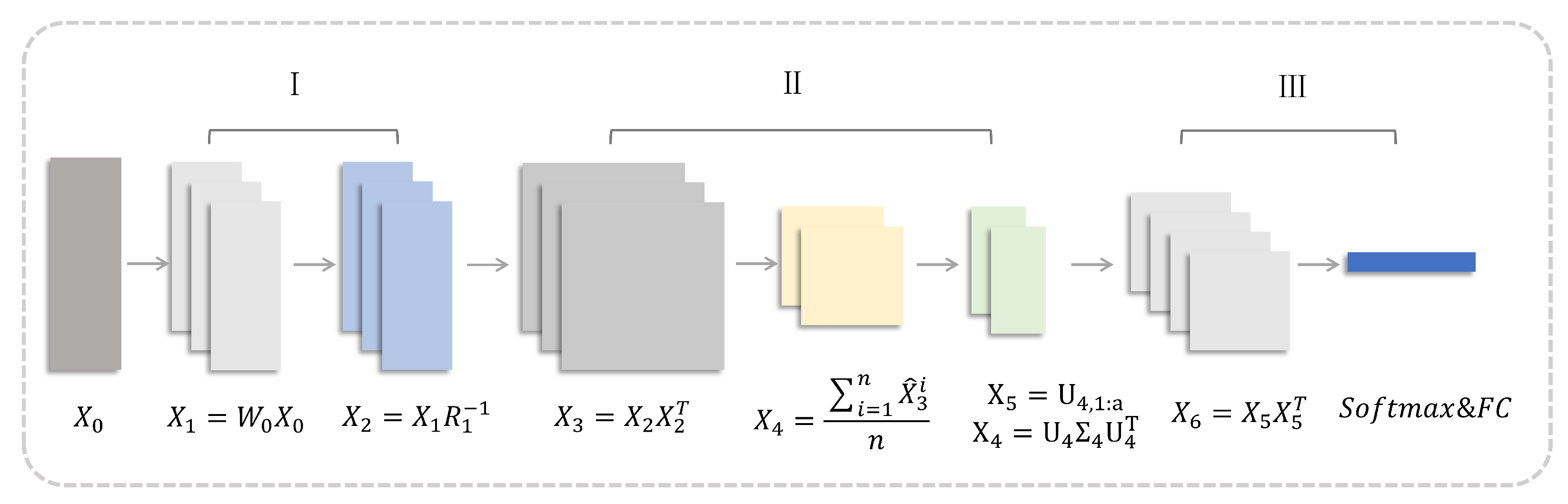
Figure 2 is an illustration of the structure of GrNet. Table 1 lists the mapping functions of each layer in GrNet and the corresponding layers between the convolutional neural network and GrNet.

2.2. Knowledge Distillation

In a classification problem, the model maps the input features to a point in the label space, and in deep neural networks, this is mostly achieved by a fully connected layer. If all samples of a class are mapped to the same point in the label space, information about intra-class variance and inter-class distances will be lost. Furthermore, although incorrect labels have different probability distributions, they are ignored when the true labels are selected. Hinton et al. [36] proposed the knowledge distillation that can distill the knowledge in an ensemble into a small model by using “soft targets”. The soft targets are the probabilities of different classes in the cumbersome models that can provide more information than the traditional ground truth (also known as hard target). The soft targets obtained from the large size teacher network (TNet) are applied to train the small size student network (SNet) through knowledge distillation to preserve the probability distribution between different incorrect labels. Therefore, the SNet imitates the training process of the TNet through knowledge distillation to adjust the network weights and achieves better performance than by training SNet only.
The softmax layer can convert the logit, z i , into the probability of i t h class, q i , as the following way:
q i = exp ( z i ) j exp ( z j )
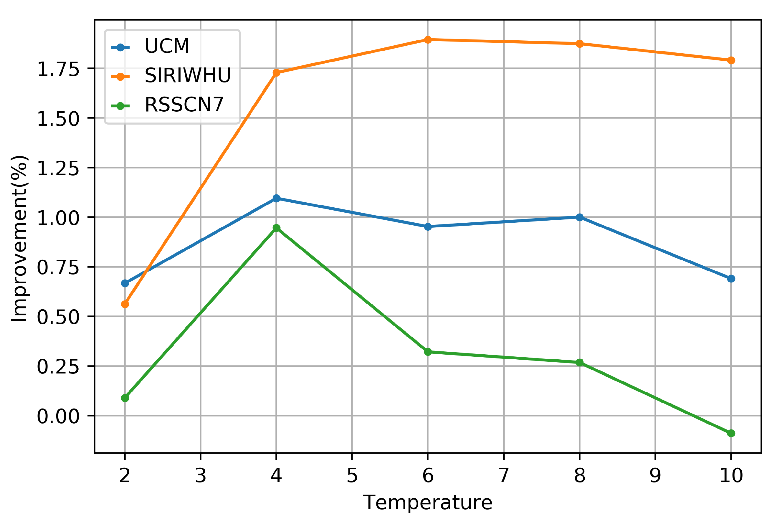
The knowledge distillation introduces a temperature parameter, t, to the softmax layer, which controls probability distribution between different classes. The probability differences between classes tend to be smaller with higher temperatures. As the temperature tends to infinity, the probability of each class tends to be equal. Through the adjustment of parameter t, the mapping curve of the softmax layer is smoother. The soft target q t i is computed as below:
q t i = exp ( z i / t ) j exp ( z j / t )
Obviously, when t is equal to 1, the soft target q t i equals q i . Instead of letting q i fit to hard target only, the knowledge distillation enables the student networks to get the knowledge that the teacher networks have already obtained by narrowing the difference between the soft targets of A and B. From a teaching perspective, a hard target is like a standard answer and a soft target is like the teacher’s experience. With the help of the teacher, students can acquire knowledge faster and better. As a result, the small network can obtain higher accuracy by using both soft targets and hard targets.
At present, there are two ideas for knowledge distillation. One is to perform knowledge distillation at the output end of the network, which is also called goal-driven knowledge distillation. The classic example of this is the distillation framework in [36], and another extension to it is ProjectionNet [37]. The other is to perform knowledge distillation in the middle layer of the network, which is also called feature matching knowledge distillation. FitNets [38] defines the hint layer and guided layer in the middle layer of TNet and SNet, respectively. The guided layer learns from the hint layer by adding a mean square loss between them in training. In [39], the authors use the attention maps of the middle layers of TNet and SNet to calculate the loss. Similar to this is the use of Gram matrices rather than the attention maps in [40]. Heo et al. [41] propose a new designed margin ReLU activation and a new distillation feature position. Other recent methods of knowledge distillation include [42,43,44,45], etc.
To sum up, the key of knowledge distillation is to break up the original supervision information compressed to one point, which is a simple way to make up for the insufficient supervision signal of the classification problem. It increases the prior knowledge obtained through soft targets, reduces the search space of the network, so as to obtain better generalization ability and accelerate the convergence speed of the network.

2.3. Overview of the Proposed Method

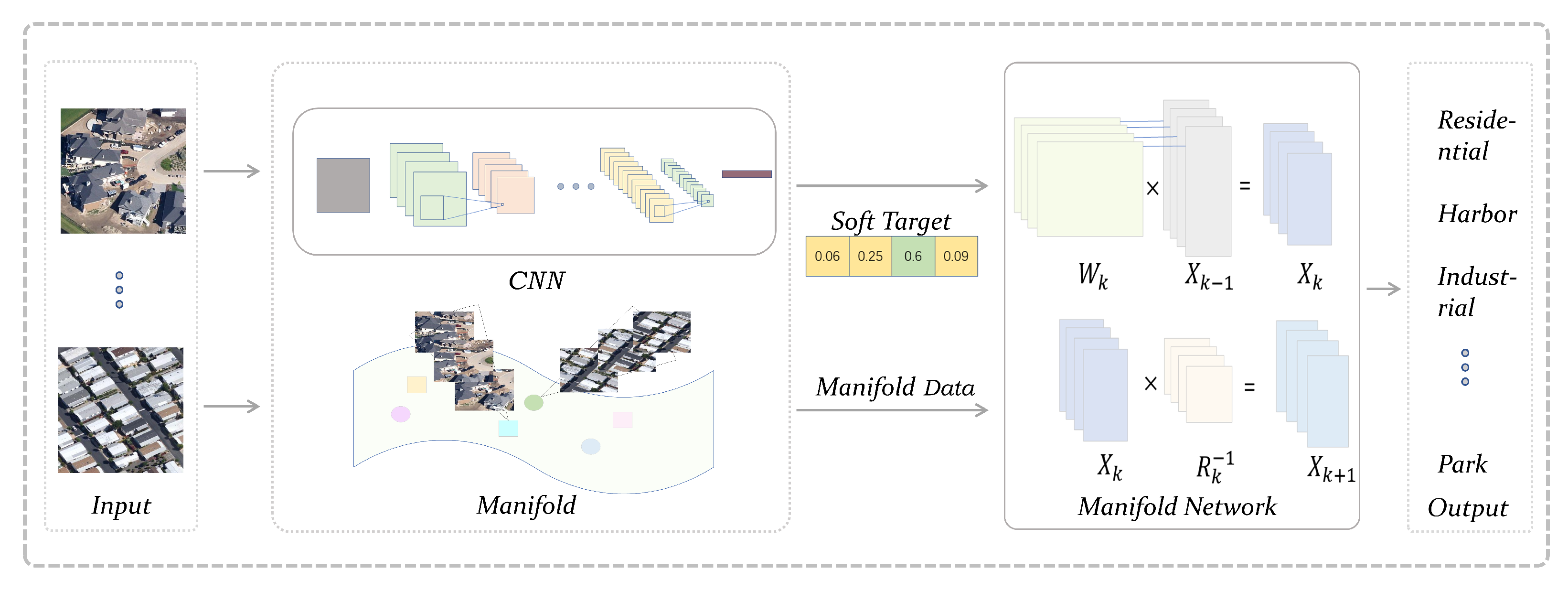
Figure 3 illustrates the way that our proposed method works. Our method consists of two flows. One is the training of traditional convolutional neural networks, and the other is the processing of the manifold network.
The remote sensing images are fed into the convolutional neural network which is called the teacher network first. The teacher network can get knowledge from a mass of data and store the knowledge in the soft targets that we use later. The input images require preprocessing because the manifold network has a special input format. In this paper, an effective approach is proposed to transform the original remote sensing images into the points in the Grassmann manifold, which is the input space of the manifold network. Then the manifold data is fed into the manifold network. Both soft targets and hard targets are used as supervisory information for training the manifold network. Finally, the resulting model can converge faster and predict more accurately than the model trained without knowledge distillation.

2.4. Training Manifold Network by Knowledge Distillation

Knowledge distillation can transfer the learning ability of a large network to a small network. The condition for distillation is that the partial structure of the student network (SNet) corresponds functionally to that of the teacher network (TNet). However, the manifold networks are structurally incompatible with the convolutional neural networks, leading to the difficulty of distillation between them. The output layers of the two networks are both fully connected layers, hence we choose to distill the knowledge on the top of networks.
First, the teacher network is trained with the original image as input, at which time t is equal to 1. The trained teacher network is cumbersome, but it has a good generalization of data. Then t is changed to be greater than 1 and we can obtain a soft target for each original image, which contains more information about the input image. In the meantime, the original images are transformed into Grassmannian data. The approach of transformation will be introduced later. Then we input the Grassmannian data into the student network. During training, the student network has two softmax layers with different temperatures, one with t equal to 1 and the other with t greater than 1. Therefore, the network has two outputs, a soft target and a hard target, and correspondingly two loss functions. We write the expression for soft target and hard target in the form of a vector as follows:
y s o f t ( z ) = e z / t ( e z / t ) · 1
y h a r d ( z ) = e z ( e z ) · 1
where z is the column vector of logit, ( ) is transposition of vector, 1 is column vector with all elements of 1, y s o f t and y h a r d are soft target and hard target respectively. Then we substitute the logit z with specific network structures as follows:
z S = M a n i N e t ( T r a n s ( x ) )
z T = C o n v N e t ( x )
where T r a n s represents the preprocessing of the input data, the M a n i N e t and C o n v N e t represent the manifold networks and convolutional neural networks respectively, x is the original input, and the superscripts S and T refer to student networks and teacher networks respectively.
The first loss function is the standard cross entropy between the soft targets of two networks, as follows:
L s o f t = C ( y s o f t T , y s o f t S )
where y s o f t T and y s o f t S are the soft targets of the teacher network and student network respectively, C is the standard cross entropy.
Another loss function is the standard cross entropy between the ground truth and hard target, as follows:
L h a r d = C ( y h a r d S , y )
where the y h a r d S is hard target of the student network.
These two loss functions form the final loss function through a weighting coefficient α . As a result, the student network can learn weights by the ground truth, and meanwhile, the knowledge learned from the teacher networks can correct the learning direction and improve the accuracy of the small model. The effect of the true labels and the teacher network on the final training results can be controlled by the α . The final loss function is formulated as follows:
= α L s o f t + 1 α L h a r d
The convolution is a linear operation, so the activation function is used to add nonlinear fitting capability. The convolutional neural network is very deep to obtain good data generalization ability, leading to the cumbersome model. However, the manifold network is defined in the non-Euclidean space, including its inputs and internal operations. The nonlinearity of the operations on the curve manifold leads to better spatial transformation capability and data fitting ability, meaning that the manifold network can achieve better results with fewer layers. With the help of knowledge distillation, we further enhance the performance of the manifold network by transferring the information in the soft targets of the cumbersome model.

Data Preprocessing

We choose GrNet as the manifold network in this paper. The GrNet is designed for Grassmannian data, so the images must be preprocessed before they are fed into the network. In face video recognition, a series of consecutive frames are sampled from the video, and the human face is extracted from the original video frame by using some face extraction algorithm. Therefore, these human face frames have similar patterns. A fixed number of images can be modeled as a linear subspace by extracting features from images, putting them together and then orthogonalizing them. However, there is a difference between human face videos and remote sensing scene images. The face images that belong to a person are very similar because they are consecutive frames extracted from the video. However, there may be a big difference for remote sensing scene images in a category. In general, for classification problems, our task is to label each image rather than classify a group of images into a category. Therefore, the above method is no longer applicable. In this paper, we propose a new method to represent a single image as a linear subspace as follows:
(1)
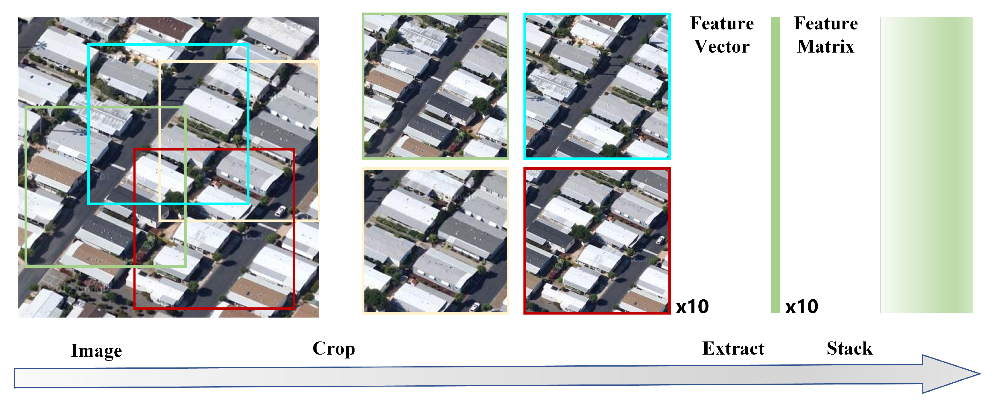
Crop and Stack. An image is randomly cut into m subgraphs first. Then we extract a feature of fixed dimension for each subgraph. The m feature vectors are stacked to form a feature matrix. This process is shown in Figure 4. In this paper, the feature extraction method is the neural network. In our experiment, we set the dimension of the feature to 512 and m to 10. As a result, each image can generate a feature matrix whose shape is 512 × 10 .
(2)
Divide the datasets. To ensure that the overall distribution of the training sets and test sets is consistent, each category in the datasets is divided into training sets and test sets in a fixed proportion.
(3)
PCA dimensionality reduction. Firstly, PCA dimension reduction is carried out on the training data, and the eigenvectors corresponding to k features with the largest eigenvalues are selected to form the eigenmatrix P. Then the eigenmatrix P obtained from the training set is used to reduce the dimension of the data of the training set and the test set. The dimension is reduced to 400 in our experiment, so the shape of the feature matrix becomes 400 × 10 .
(4)
Generate linear subspace. The feature matrix obtained in (3) is transformed into the orthogonal matrix by singular value decomposition(SVD). An orthogonal matrix is a linear subspace that is a point in the Grassmann manifold and also the input to GrNet.

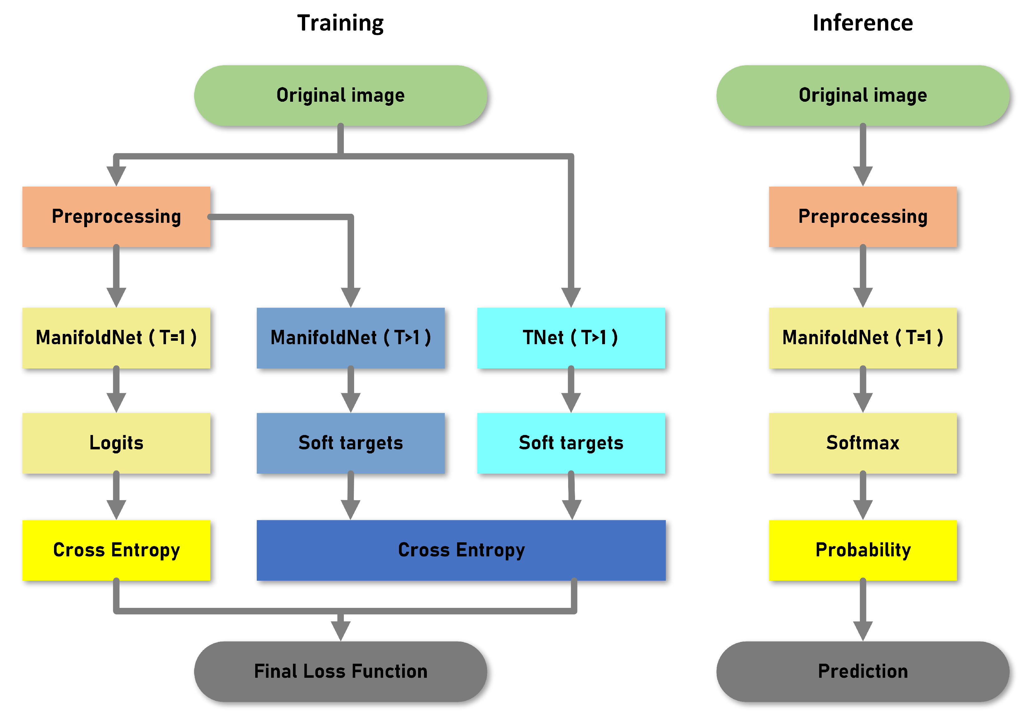
2.5. The Flow of Proposed Method

The entire algorithm flowchart is shown in Figure 5. First, input the original optical remote sensing images into a trained teacher network with a distillation temperature greater than 1 to get the soft targets. At meanwhile, each image is preprocessed as mentioned above to generate the manifold data. The processed data is entered into the manifold network which has two softmax layers. The first softmax layer with a temperature greater than 1 outputs the soft targets, which calculates the cross-entropy loss with the above soft targets. The second softmax layer with temperature equals 1 outputs logits, and the cross-entropy loss between the ground truth and these hard targets is computed. The final loss function is composed of these two losses and we train the network with a backpropagation algorithm. At inference, the processed images are input into the manifold network with the temperature equals 1, and the prediction results are output according to the obtained probability of each class.

3. Results

In this section, we first introduce three datasets used for the experiments. And then, some parameters in the experiments are discussed in detail here. Finally, we perform our method on these three remote sensing image datasets and the experimental results will be displayed. In addition, we discuss the effects of α and distillation temperature T.

3.1. DataSet

We choose four remote sensing scene classification datasets, namely UC Merced Land Use [46] (UCM for short), SIRI-WHU [8,47], RSSCN7 [48] and Aerial Image Dataset (AID) [49]. The number of categories in the four datasets is different, from 7 to 30, which can make the method in this paper more universal. They have rich image information and features, and complex texture structures, which bring a great challenge to classification tasks.

3.1.1. UC Merced Land Use Dataset

The images of the UC Merced Land Use dataset are selected from the USGS National Map Urban Area Imagery collection and cover areas across the United States. The UC Merced Land Use dataset includes 21 categories, and each aerial scene contains 100 images, whose size is 256 × 256 pixels. They have a resolution of 1 foot per pixel. Figure 6 shows some examples of different categories.

3.1.2. SIRI-WHU Dataset

The SIRI-WHU dataset comes from Google Earth, mainly covering urban areas in China, and was designed by RS_IDEA Group of Wuhan University. It is composed of 12 scenes classes, and each category contains 200 images. The 12 scene classes include agriculture, commercial, harbor, idle land, industrial, meadow, overpass, park, pond, residential, river and water as Figure 7. The spatial resolution is 2 meters, and images have a size of 200 × 200 pixels.

3.1.3. RSSCN7 Dataset

The RSSCN7 dataset is quite challenging because of the diversity of scene images captured in different seasons and different weather, and sampled at different scales. There are 2800 remote sensing images from 7 different typical scenes, namely grass, field, industry, river&lake, forest, resident and parking. For each category, 400 images were taken from Google Earth, sampled on four different scales, 100 images per scale. The size of each image is 400 × 400 pixels. The samples from the seven categories are shown in Figure 8.

3.1.4. Aerial Image Dataset

The AID is a remote sensing image dataset containing 30 categories of scene images, each with approximately 220–420 images. The entire dataset consists of 10,000 images with a pixel size of 600 × 600. The samples in AID have different spatial resolutions, which is more challenging for scene classification.
For the first three datasets, we randomly choose 20% of each class as the test set so that the training set and test set can have the same distribution. And for the AID dataset, 20% and 50% of the data are used as the training sets respectively. Table 2 shows the number of images in the test set and the training set in the four remote sensing scene classification datasets.

3.2. Experiment Setup

In this experiment, GrNet2B [28] is selected as student net due to its outstanding performance. GrNet2B is composed of two Projection blocks, two Pooling blocks and one Output block. According to the research [50], the modified GrNet without Pooling Block can achieve higher accuracy, but it’s significant to maintain the complete structure to reveal Grassmann manifold and helpful for feature work based on vanilla GrNet. The sizes of GrNet-2B weights are set to 400 × 300 and 150 × 100 to fit with the datasets and our method. The ResNet34 is chosen as the teacher network. A softmax layer with the temperature mentioned above is added to the end of ResNet34, which can generate soft targets so as to fit knowledge distillation. We set the mini-batch size to 32 and the optimization algorithm is Stochastic Gradient Descent (SGD). The momentum and weight decay are set to 0 by default. The learning rate is important and we set it to 5 for the student network, 0.05 for the teacher network and 1 for the distillation process. The learning rate of GrNet is halved at the 5th, 10th, and 35th epoch. All experiments are run on two NVIDIA TITAN X (Pascal) GPUs with 12Gb of memory.
We use overall accuracy and the confusion matrix to evaluate the results of scene classification. The default temperature T of knowledge distillation is set to 4, and the default weighted coefficient α is set to 0.4. To ensure the reliability of the experimental results, the experiments were repeated 10 times for the first three datasets and three times for the AID dataset. The mean value is taken as the final result, and the mean square deviation is also reported. As for more details about knowledge distillation, we will discuss it below.

3.3. Experimental Analysis and Results

In order to illustrate the effectiveness of our method, the experiments are carried on four remote sensing scene datasets, namely UC Merced Land Use, SIRI-WHU, RSSCN7 and AID datasets.

3.3.1. Results on UC Merced Land Use Dataset

In order to figure out the effect of different networks on knowledge distillation, we add the experiment of ResNet50 on this dataset. The experimental results on the UC Merced Land Use dataset are listed in Table 3. As can be seen from the table, the GrNet2B trained by knowledge distillation with the ResNet34 improves the accuracy by 1.09% compared with the GrNet2B trained by the ground truth alone. Although ResNet34 is more accurate than GrNet2B, the results are still excellent considering the size difference between the two models. With a 92.96% reduction in model size, there was only a 7.37% reduction in model accuracy, which can solve the problem of deep learning deployment on resource-limited embedded devices. GrNet2B has only 0.02G of Mac computation, which is much less than 3.15G and 3.52G of that of ResNet. The significant reduction in calculations is due to the format of the manifold data, which lies on the curved manifold. Also because of the special input data, the Grassmann manifold network is mostly based on matrix operations, resulting in less computational effort. When ResNet50 is selected as the teacher network, knowledge distillation can achieve a 2.31% improvement in accuracy. Therefore, the selection of the teacher networks allows for a wider range of possibilities.
Furthermore, the training process using knowledge distillation is greatly accelerated. We can see from Figure 9 that with plain training, the model needs more than 10 epochs to converge to high accuracy. However, using knowledge distillation, the model only needs 5 epochs to reach a high accuracy, which benefits from the prior knowledge from the teacher network.

3.3.2. Results on SIRI-WHU, RSSCN7 and AID Dataset

The knowledge distillation is also performed on the SIRI-WHU, RSSCN7 and AID datasets. The classification results of vanilla GrNet and distilled manifold network on the three remote sensing scene datasets are shown in Table 4. On the SIRI-WHU dataset, distilled GeNet2B can achieve 1.73% accuracy improvement compared with the vanilla GrNet2B. Compared with ResNet34, the accuracy of the distilled model is reduced by only 9.10% when the model size is reduced by 93.80%. On the RSSCN7 dataset, the accuracy of the proposed method is improved by 0.95% compared with the vanilla GrNet2B. Compared to ResNet34, the accuracy of distilled GrNet2B is only reduced by 9.03% with a 94.27% reduction in model size. On the AID dataset, the proposed method improved the accuracy by 0.37% over vanilla GrNet2B. The distilled GrNet2B has 11.43% lower accuracy than ResNet34, but its model size has been reduced by 92.11%. Model size and accuracy are paradoxical, so we need to find a trade-off between the two. With such a large drop in model size, the accuracy of our method remains competitive.
We list some of the misclassified images, as shown in Figure 10. These images are so similar that humans can make a mistake in distinguishing between them. The confusion matrixes obtained by testing on the UCM, SIRI-WHU and RSSCN7 datasets respectively are shown in the left column of Figure 11. It can be seen that most images are correctly classified. The reason for misclassification is that images have similarities in the different classes, and images may have a large difference in the same class.
The right column of Figure 11 is the results of ten random repeat experiments on UC Merced Land Use, SIRI-WHU and RSSCN7 datasets, respectively. The blue line represents the accuracy of the vanilla GrNet and the green line represents the accuracy of the distilled GrNet. As is shown in Figure 11, the green lines are almost always above the blue lines in all three figures. Therefore, the method proposed in this paper has good robustness.

3.3.3. Comparison Experiments with Shallow CNNs

We also conduct a comparison experiment using a small CNN. The small CNN consists of two convolutional layers and a fully connected layer. Each convolutional layer is followed by an activation function and a max pooling layer. The structure of this simple CNN is similar to that of GrNet2B, and the number of parameters in the CNN is also on the same order of magnitude as it. The simple CNN is trained on the four datasets and the experimental results are listed in Table 5. Obviously, the shallow CNN has very poor classification capabilities. Although the shallow CNN is slightly larger than GrNet2B, the classification accuracy of this CNN is significantly lower than that of GrNet. As a result, our model has excellent performance at the same size level.

3.3.4. Effect of Parameters

Property of Parameter T. As mentioned above, the parameter T, i.e., distillation temperature, is important for the experiment because it determines the level of information utilization in negative labels. Therefore, we test different temperatures T and repeat all experiments at a series of values, that is, from 2 to 10 in intervals of 2. And the results are listed in Table 6. The vanilla GrNet is used as the baseline. The visualization of the data above is presented in Figure 12, and the ordinate is the difference between the accuracy of the model with temperature x and the baseline. As we can see in Figure 12, as the temperature rises, the accuracy first rises and then falls in general. The best performance of the knowledge distillation appears at different temperatures on the three remote sensing datasets. On the UCM and RSSCN7 datasets, the accuracy is highest when T is 4. As for the SIRI-WHU dataset, the model with a temperature of 6 achieves the best performance. There are many differences in texture structures and image features among the three datasets, so it’s reasonable that different datasets have different optimal temperatures. When we draw them in a line chart, it’s easy to find that the optimal temperature is approximately concentrated from 4 to 6. Therefore, the other experiments will be conducted at a temperature of 4. When the temperature is so low that it approaches 1, the softmax layers become naive, and the difference between positive and negative labels is too large. When the temperature is very high, we can see from the softmax formula with the temperature that the difference between all labels, including positive labels and negative labels, is very small, so the ability to distinguish between different categories is reduced.
Property of Parameter α . The knowledge distillation utilizes the information learned from the teacher network and student network. The teacher network can learn more knowledge than the student network from a lot of data and store it in the soft targets, which is used by the student network. On the other side, the student network gets information from the ground truth at the same time. As mentioned above, α is the weighted coefficient between the two loss functions, i.e., L s o f t and L h a r d . The L h a r d uses the original supervised information to limit the scope of the solution space, and the L s o f t contains more prior knowledge learned from the cumbersome teacher model. Therefore, α can manipulate which of the two types of information is more dominant in guiding the convergence of the network.
In order to figure out the effect of α , we experiment on three datasets with different α . The value of α is from 0 to 1 in intervals of 0.1 in all datasets. According to Equation (10), the vanilla GrNet is the special case of distillation when the α is 0. The results are listed in Table 7. The Figure 13 shows that the optimal α is approximately between 0.2 and 0.5. When α is greater than 0.5, the accuracy will decrease as α increases. When the α is equal to 1, the loss function is only composed of L s o f t , that is, the training process is completely controlled by the prior knowledge of the teacher network. Due to the lack of supervision of the ground truth, incorrect knowledge from the teacher network will also be passed to the student network, which leads to the decline of the accuracy of the model. Consequently, we get the conclusion that the ground truth plays a more important role in training the Grassmann manifold network on these three datasets. The soft targets can assist in guiding the training of the small network and correct the direction of network convergence.

4. Discussion

We have conducted experiments on three different remote sensing datasets and the experimental results show that the method proposed in this paper is effective. The method in this paper is not as good as convolutional neural networks, but the lower loss of accuracy is rewarded with a huge saving in model size. The proposed method is more feasible and valuable when considering the environment in which the neural network is deployed. In addition to higher accuracy rates, faster training is also an advantage of this method. As there are many pre-trained models published by other companies or institutions, the training cost of our proposed method is acceptable.
There are two hyperparameters in our experiment, namely temperature and α . Temperature controls the relative size of the different labels to each other and thus affects the utilization of the information they contain. When the temperature is too low, the gap between the positive and negative labels will cover the gap between the different negative labels. When the temperature is too high, the gap between all tables becomes quite small, and there is a great loss of information. Furthermore, Our experiment also gives a conclusion that is consistent with this. The α controls the proportion of the ground truth and the teacher network’s contributions to training. As can be seen from the experimental results, when α equals 0 or 1, the accuracy of the model cannot reach the highest, which indicates that training only by ground truth or soft targets is not enough. In another way, we also know that the addition of either of these two has a positive effect on the performance of the model. The optimal value of α is 0.4, so we think that ground truth plays a more important role than soft targets in the experiments of this paper. This also shows that the innovative point of the article is valid.

5. Conclusions

In this paper, we introduced a novel method to use knowledge distillation to train the Grassmann manifold network, which also breaks the isolation between convolutional neural networks and manifold networks. Our approach is general and applicable to other convolutional neural networks and manifold networks. The advantages of deep convolutional neural networks and shallow manifold networks were combined to improve the accuracy of small networks. The size of the model has been significantly reduced while maintaining considerable performance, which helps in the deployment of deep learning models on resource-limited devices such as embedded devices. We propose a preprocessing method that converts a single image into a point in a Grassmannian manifold. Our method was performed on three remote sensing scene classification datasets, and the results show that our method effectively improves the accuracy. Some details about the effects of parameters T and α were discussed above. In the future, we will explore the more general manifold networks to improve the generality of the manifold network and simplify its structure.

Author Contributions

Methodology, L.T. and Z.W.; software, Z.W.; writing—original draft preparation, Z.W., B.H. and L.T.; writing—review and editing, Z.W. and C.H.; Project administration, C.H., D.W. and D.L. All authors have read and agreed to the published version of the manuscript.

Funding

This research was funded by the National Key Research and Development Program of China (No. 2016YFC0803000) and the National Natural Science Foundation of China (No. 41371342).

Institutional Review Board Statement

Not applicable.

Informed Consent Statement

Not applicable.

Data Availability Statement

No new data were created or analyzed in this study. Data sharing is not applicable to this article.

Conflicts of Interest

The authors declare no conflict of interest.

Abbreviations

The following abbreviations are used in this manuscript:
CNNConvolutional Neural Network
CIFARCanadian Institute for Advanced Research
SGDStochastic Gradient Descent
GrNetGrassmann network
SIFTScale-Invariant Feature Transform
ReLURectified Linear Unit
SNetStudent network
TNetTeacher network
LLELocally Linear Embedding
ISOMAPIsometric feature mapping
LELaplacian Eigenmaps
SPDSymmetric Positive Definite

References

  1. Xu, Z.; Zhang, W.; Zhang, T.; Li, J. HRCNet: High-resolution context extraction network for semantic segmentation of remote sensing images. Remote Sens. 2021, 13, 71. [Google Scholar] [CrossRef]
  2. Ouyang, S.; Li, Y. Combining deep semantic segmentation network and graph convolutional neural network for semantic segmentation of remote sensing imagery. Remote Sens. 2021, 13, 119. [Google Scholar] [CrossRef]
  3. Li, K.; Wan, G.; Cheng, G.; Meng, L.; Han, J. Object detection in optical remote sensing images: A survey and a new benchmark. ISPRS J. Photogramm. Remote Sens. 2020, 159, 296–307. [Google Scholar] [CrossRef]
  4. Yang, K.; Xia, G.S.; Liu, Z.; Du, B.; Yang, W.; Pelillo, M.; Zhang, L. Asymmetric Siamese Networks for Semantic Change Detection in Aerial Images. IEEE Trans. Geosci. Remote. Sens. 2021, 1–18. [Google Scholar] [CrossRef]
  5. Maxwell, A.E.; Bester, M.S.; Guillen, L.A.; Ramezan, C.A.; Carpinello, D.J.; Fan, Y.; Hartley, F.M.; Maynard, S.M.; Pyron, J.L. Semantic Segmentation Deep Learning for Extracting Surface Mine Extents from Historic Topographic Maps. Remote Sens. 2020, 12, 4145. [Google Scholar] [CrossRef]
  6. Kalajdjieski, J.; Zdravevski, E.; Corizzo, R.; Lameski, P.; Kalajdziski, S.; Pires, I.M.; Garcia, N.M.; Trajkovik, V. Air pollution prediction with multi-modal data and deep neural networks. Remote Sens. 2020, 12, 4142. [Google Scholar] [CrossRef]
  7. Risojević, V.; Babić, Z. Unsupervised quaternion feature learning for remote sensing image classification. IEEE J. Sel. Top. Appl. Earth Obs. Remote Sens. 2016, 9, 1521–1531. [Google Scholar] [CrossRef]
  8. Zhu, Q.; Zhong, Y.; Zhao, B.; Xia, G.S.; Zhang, L. Bag-of-visual-words scene classifier with local and global features for high spatial resolution remote sensing imagery. IEEE Geosci. Remote Sens. Lett. 2016, 13, 747–751. [Google Scholar] [CrossRef]
  9. Zhu, Q.; Zhong, Y.; Zhang, L.; Li, D. Scene classification based on the fully sparse semantic topic model. IEEE Trans. Geosci. Remote Sens. 2017, 55, 5525–5538. [Google Scholar] [CrossRef]
  10. Bian, X.; Chen, C.; Tian, L.; Du, Q. Fusing local and global features for high-resolution scene classification. IEEE J. Sel. Top. Appl. Earth Obs. Remote Sens. 2017, 10, 2889–2901. [Google Scholar] [CrossRef]
  11. Sridharan, H.; Cheriyadat, A. Bag of lines (BoL) for improved aerial scene representation. IEEE Geosci. Remote Sens. Lett. 2014, 12, 676–680. [Google Scholar] [CrossRef]
  12. Bahmanyar, R.; Cui, S.; Datcu, M. A comparative study of bag-of-words and bag-of-topics models of EO image patches. IEEE Geosci. Remote Sens. Lett. 2015, 12, 1357–1361. [Google Scholar] [CrossRef] [Green Version]
  13. Marmanis, D.; Datcu, M.; Esch, T.; Stilla, U. Deep learning earth observation classification using ImageNet pretrained networks. IEEE Geosci. Remote Sens. Lett. 2015, 13, 105–109. [Google Scholar] [CrossRef] [Green Version]
  14. Cheng, G.; Li, Z.; Yao, X.; Guo, L.; Wei, Z. Remote sensing image scene classification using bag of convolutional features. IEEE Geosci. Remote Sens. Lett. 2017, 14, 1735–1739. [Google Scholar] [CrossRef]
  15. Yuan, B.; Han, L.; Gu, X.; Yan, H. Multi-deep features fusion for high-resolution remote sensing image scene classification. Neural Comput. Appl. 2021, 33, 2047–2063. [Google Scholar] [CrossRef]
  16. Xu, K.; Huang, H.; Deng, P. Remote Sensing Image Scene Classification Based on Global-Local Dual-Branch Structure Model. IEEE Geosci. Remote. Sens. Lett. 2021, 1–5. [Google Scholar] [CrossRef]
  17. Xu, K.; Huang, H.; Deng, P.; Shi, G. Two-stream feature aggregation deep neural network for scene classification of remote sensing images. Inf. Sci. 2020, 539, 250–268. [Google Scholar] [CrossRef]
  18. Xu, K.; Huang, H.; Deng, P.; Li, Y. Deep Feature Aggregation Framework Driven by Graph Convolutional Network for Scene Classification in Remote Sensing. IEEE Trans. Neural Netw. Learn. Syst. 2021, 1–15. [Google Scholar] [CrossRef]
  19. Bi, Q.; Qin, K.; Zhang, H.; Xia, G.S. Local Semantic Enhanced ConvNet for Aerial Scene Recognition. IEEE Trans. Image Process. 2021, 30, 6498–6511. [Google Scholar] [CrossRef]
  20. Li, L.; Han, J.; Yao, X.; Cheng, G.; Guo, L. DLA-MatchNet for few-shot remote sensing image scene classification. IEEE Trans. Geosci. Remote Sens. 2020, 9, 7844–7853. [Google Scholar] [CrossRef]
  21. Deng, P.; Xu, K.; Huang, H. When CNNs Meet Vision Transformer: A Joint Framework for Remote Sensing Scene Classification. IEEE Geosci. Remote Sens. Lett. 2021, 1–5. [Google Scholar] [CrossRef]
  22. Glorot, X.; Bordes, A.; Bengio, Y. Deep sparse rectifier neural networks. In Proceedings of the Fourteenth International Conference on Artificial Intelligence and Statistics, Lauderdale, FL, USA, 11–13 April 2011; pp. 315–323. [Google Scholar]
  23. Kingma, D.P.; Ba, J. Adam: A method for stochastic optimization. arXiv 2014, arXiv:1412.6980. [Google Scholar]
  24. Mugavin, M.E. Multidimensional scaling: A brief overview. Nurs. Res. 2008, 57, 64–68. [Google Scholar] [CrossRef]
  25. Tenenbaum, J.B.; De Silva, V.; Langford, J.C. A global geometric framework for nonlinear dimensionality reduction. Science 2000, 290, 2319–2323. [Google Scholar] [CrossRef] [PubMed]
  26. Roweis, S.T.; Saul, L.K. Nonlinear dimensionality reduction by locally linear embedding. Science 2000, 290, 2323–2326. [Google Scholar] [CrossRef] [PubMed] [Green Version]
  27. Belkin, M.; Niyogi, P. Laplacian eigenmaps for dimensionality reduction and data representation. Neural Comput. 2003, 15, 1373–1396. [Google Scholar] [CrossRef] [Green Version]
  28. Huang, Z.; Wu, J.; Van Gool, L. Building deep networks on Grassmann manifolds. arXiv 2016, arXiv:1611.05742. [Google Scholar]
  29. Huang, Z.; Van Gool, L. A riemannian network for spd matrix learning. In Proceedings of the Thirty-First AAAI Conference on Artificial Intelligence, San Francisco, CA, USA, 4–9 February 2017. [Google Scholar]
  30. Chakraborty, R.; Bouza, J.; Manton, J.; Vemuri, B.C. Manifoldnet: A deep neural network for manifold-valued data with applications. IEEE Trans. Pattern Anal. Mach. Intell. 2020, 1. [Google Scholar] [CrossRef]
  31. Fréchet, M. Les éléments aléatoires de Nature Quelconque Dans un Espace Distancié; Annales de l’institut Henri Poincaré: Durham, NC, USA, 1948; pp. 215–310. [Google Scholar]
  32. Absil, P.A.; Mahony, R.; Sepulchre, R. Optimization Algorithms on Matrix Manifolds; Princeton University Press: Princeton, NJ, USA, 2009. [Google Scholar]
  33. Ionescu, C.; Vantzos, O.; Sminchisescu, C. Training deep networks with structured layers by matrix backpropagation. arXiv 2015, arXiv:1509.07838. [Google Scholar]
  34. Liu, M.; Wang, R.; Huang, Z.; Shan, S.; Chen, X. Partial least squares regression on grassmannian manifold for emotion recognition. In Proceedings of the 15th ACM on International Conference on Multimodal Interaction, Sydney, Australia, 9–13 December 2013; pp. 525–530. [Google Scholar]
  35. Liu, M.; Wang, R.; Li, S.; Shan, S.; Huang, Z.; Chen, X. Combining multiple kernel methods on riemannian manifold for emotion recognition in the wild. In Proceedings of the 16th International Conference on Multimodal Interaction, Istanbul, Turkey, 12–16 November 2014; pp. 494–501. [Google Scholar]
  36. Hinton, G.; Vinyals, O.; Dean, J. Distilling the knowledge in a neural network. arXiv 2015, arXiv:1503.02531. [Google Scholar]
  37. Ravi, S. Projectionnet: Learning efficient on-device deep networks using neural projections. arXiv 2017, arXiv:1708.00630. [Google Scholar]
  38. Romero, A.; Ballas, N.; Kahou, S.E.; Chassang, A.; Gatta, C.; Bengio, Y. Fitnets: Hints for thin deep nets. arXiv 2014, arXiv:1412.6550. [Google Scholar]
  39. Zagoruyko, S.; Komodakis, N. Paying more attention to attention: Improving the performance of convolutional neural networks via attention transfer. arXiv 2016, arXiv:1612.03928. [Google Scholar]
  40. Yim, J.; Joo, D.; Bae, J.; Kim, J. A gift from knowledge distillation: Fast optimization, network minimization and transfer learning. In Proceedings of the IEEE Conference on Computer Vision and Pattern Recognition, Honolulu, HI, USA, 21–26 July 2017; pp. 4133–4141. [Google Scholar]
  41. Heo, B.; Kim, J.; Yun, S.; Park, H.; Kwak, N.; Choi, J.Y. A Comprehensive Overhaul of Feature Distillation. In Proceedings of the IEEE/CVF International Conference on Computer Vision (ICCV), Seoul, Korea, 27 October–2 November 2019. [Google Scholar]
  42. Huang, Z.; Wang, N. Like what you like: Knowledge distill via neuron selectivity transfer. arXiv 2017, arXiv:1707.01219. [Google Scholar]
  43. Kim, J.; Park, S.; Kwak, N. Paraphrasing complex network: Network compression via factor transfer. arXiv 2018, arXiv:1802.04977. [Google Scholar]
  44. Xu, Z.; Hsu, Y.C.; Huang, J. Training shallow and thin networks for acceleration via knowledge distillation with conditional adversarial networks. arXiv 2017, arXiv:1709.00513. [Google Scholar]
  45. Furlanello, T.; Lipton, Z.; Tschannen, M.; Itti, L.; Anandkumar, A. Born again neural networks. In Proceedings of the International Conference on Machine Learning, PMLR, Stockholm, Sweden, 10–15 July 2018; pp. 1607–1616. [Google Scholar]
  46. Yang, Y.; Newsam, S. Bag-of-visual-words and spatial extensions for land-use classification. In Proceedings of the 18th Sigspatial International Conference on Advances in Geographic Information Systems, San Jose, CA, USA, 2–5 November 2010; pp. 270–279. [Google Scholar]
  47. Zhao, B.; Zhong, Y.; Xia, G.S.; Zhang, L. Dirichlet-derived multiple topic scene classification model for high spatial resolution remote sensing imagery. IEEE Trans. Geosci. Remote Sens. 2015, 54, 2108–2123. [Google Scholar] [CrossRef]
  48. Zou, Q.; Ni, L.; Zhang, T.; Wang, Q. Deep learning based feature selection for remote sensing scene classification. IEEE Geosci. Remote Sens. Lett. 2015, 12, 2321–2325. [Google Scholar] [CrossRef]
  49. Xia, G.S.; Hu, J.; Hu, F.; Shi, B.; Bai, X.; Zhong, Y.; Zhang, L.; Lu, X. AID: A benchmark data set for performance evaluation of aerial scene classification. IEEE Trans. Geosci. Remote Sens. 2017, 55, 3965–3981. [Google Scholar] [CrossRef] [Green Version]
  50. Tianci, L.; Zelin, S.; Yunpeng, L.; Yingdi, Z. Geometry deep network image-set recognition method based on Grassmann manifolds. Infrared Laser Eng. 2018, 47, 703002. [Google Scholar] [CrossRef]
Figure 1. Comparison of the effectiveness of linear and nonlinear transformations for data classification. The first figure (A) shows the original data distribution, the second figure (B) shows the distribution of the data after linear transformation, and the last two figures (C,D) are the distribution of the data after nonlinear transformation.
Remotesensing 13 04537 g001
Figure 2. Illustration of GrNet structure. (I): Projection Block. (II): Pooling Block. (III): Output Block.
Remotesensing 13 04537 g002
Figure 3. The overview of the proposed method. On the one hand, the images are fed into a convolutional neural network to obtain soft targets. On the other hand, they are also transformed into manifold data. The manifold network is trained with manifold data as input and soft target and hard target as supervised information.
Remotesensing 13 04537 g003
Figure 4. The illustration of first step for preprocessing. A single image is “cropped-extracted-stacked” to produce a feature matrix.
Remotesensing 13 04537 g004
Figure 5. The flow chart of our proposed method.
Remotesensing 13 04537 g005
Figure 6. Example images in 21 categories in the UC Merced Land Use dataset. (au) Agricultural, airplane, baseballdiamond, beach, buildings, chaparral, denseresidential, forest, freeway, golfcourse, harbor, intersection, mediumresidential, mobilehomepark, overpass, parkinglot, river, runway, sparseresidential, storagetanks and tenniscourt, respectively.
Remotesensing 13 04537 g006
Figure 7. Example images in 12 categories in the SIRI-WHU dataset. (al) Agriculture, commercial, harbor, idle land, industrial, meadow, overpass, park, pond, residential, river and water, respectively.
Remotesensing 13 04537 g007
Figure 8. Example images in 7 categories in the RSSCN7 dataset. (ag) Grass, field, industry, river&lake, forest, resident and parking. respectively.
Remotesensing 13 04537 g008
Figure 9. Convergence rate comparison between GrNet and Distilled GrNet.
Remotesensing 13 04537 g009
Figure 10. Some examples of misclassified images.They are denseresidential and mediumresidential, grass and field, harbor and water, industry and parking respectively.
Remotesensing 13 04537 g010
Figure 11. The confusion matrices and ten experimental results of model trained on the UCM, SIRI-WHU and RSSCN7 datasets.
Remotesensing 13 04537 g011
Figure 12. The diagram of influence of temperature T.
Remotesensing 13 04537 g012
Figure 13. The diagram of influence of α .
Remotesensing 13 04537 g013
Table 1. Mapping function of each layer in GrNet and the corresponding layer in CNN.
CNN LayerGrNet Layer f k
Convolutional LayerFRMap Layer X k = f f r ( k ) ( X k 1 ; W k ) = W k X k 1
Nonlinear Activation FunctionReorth Layer X k = f r o ( k ) ( X k 1 ) = X k 1 R k 1 1 = Q k 1 , X k 1 = Q k 1 R k 1
Average Pooling LayerProjMap Layer X k = f p m ( k ) X k 1 = X k 1 X k 1 T
ProjPooling Layer X k = f p p ( k ) ( { X ^ k 1 1 , X ^ k 1 2 , , X ^ k 1 n } ) = 1 n i = 1 n X ^ k 1 i
OrthMap Layer X k = f o m k ( X k 1 ) = U k 1 , 1 : a , X k 1 = U k 1 Σ k 1 U k 1 T
Table 2. The number of images in the test set and the training set in the three datasets.
UCMSIRI-WHURSSCN7AID
Training1680192022402000/5000
Test4204805608000/5000
Total21002400280010,000
Table 3. The accuracy of ResNet34 and ResNet50 on UC Merced Land Use datasets.
TNet#Param/MacTNet AccSNet#Param/MacSNet AccDistillation Result
ResNet3421.30 M/3.15 G98.67 ± 0.55GrNet2B1.50 M/0.02 G90.31 ± 1.0091.40  ± 0.98
ResNet5023.55 M/3.52 G98.10 ± 0.19GrNet2B1.50 M/0.02 G90.31 ± 1.0092.62 ± 0.39
Table 4. The accuracy on SIRI-WHU, RSSCN7 and AID datasets.
DatasetResNet34 (TNet)# ParamsGrNet2B (SNet)# ParamsDistillation Result
SIRI-WHU96.90 ± 0.6221.29 M86.35 ± 0.961.32 M88.08 ± 1.14
RSSCN795.77 ± 1.1421.29 M86.18 ± 1.101.22 M87.12 ± 1.14
AID91.42 ± 0.0221.29 M80.60 ± 0.001.68 M80.97 ± 0.01
Table 5. Comparison experiments with shallow CNNs on the four datasets.
DatasetShallow CNN#ParamsGrNet#Params
UCM53.813.51 M92.621.5 M
SIRI-WHU58.332.07 M88.081.32 M
RSSCN766.961.27 M87.121.22 M
AID42.764.95 M80.971.68 M
Table 6. The experimental results at different temperature on the three datasets.
T 246810
UCM90.97691.404691.261991.309690.9994
SIRI-WHU86.916688.083388.2588.229288.1459
RSSCN786.267987.124886.499986.446386.0893
Table 7. The experimental results at different α on the three datasets.
α 00.10.20.30.40.50.60.70.80.91
UCM89.7690.47691.19091.42991.42991.42991.19091.19091.19090.47690.952
SIRI-WHU87.29288.95889.16789.16788.7588.54288.12588.12587.91787.08386.458
RSSCN787.32188.03688.21488.21488.03688.03687.67987.50087.14386.78686.964
Publisher’s Note: MDPI stays neutral with regard to jurisdictional claims in published maps and institutional affiliations.

