Dual-Channel Convolutional Neural Network for Bare Surface Soil Moisture Inversion Based on Polarimetric Scattering Models

Abstract

The polarimetric synthetic aperture radar (PolSAR) can be used to obtain soil moisture by inverting scattering models at high resolution. The convolutional neural network (CNN) has been recently introduced to estimate soil roughness for PolSAR data, which need to be driven by a large amount of data. In this paper, a dual-channel CNN based on polarimetric models is proposed for soil moisture inversion, and it aims to further expand the applicable range of roughness in the X-Bragg model by integration with the integral equation model (IEM). Meanwhile, it fully utilizes the spatial information of PolSAR images to relax the number of required training samples when real data on the surface are difficult to obtain. Besides, we designed a framework based on this network. Coarse-grained inversion and fine-grained inversion of soil moisture are carried out through the qualitative classification network and the quantitative regression network, respectively. Experiments on simulated and airborne E-SAR data show that the proposed network can accurately fit the nonlinear relationship between polarization parameters and soil moisture, so as to improve the inversion accuracy with a small number of samples. In our experiments, the average inversion accuracy reached 95.39%, and the root mean square error (RMSE) of the regression network was 0.98%. This method can be applied to a wide range of soil moisture monitoring applications.

1. Introduction

Soil moisture is an important basis for assisting the development of agriculture and forestry [1,2,3]. Soil moisture is also a very important variable in the study of the terrestrial water cycle and energy cycle. It can affect not only the distribution ratio of the conversion of net radiant energy into latent heat and sensible heat, but also the ratio of precipitation into infiltration, runoff, and evaporation. Therefore, accurate acquisition of soil water content can make reasonable use of the land to improve production levels and production quality. Previously, the methods for accurately measuring soil water content were traditional methods such as time domain reflectometry (TDR) [4]. These traditional methods can accurately measure local soil moisture content. However, they require much workforce and material resources and are not suitable for large-scale soil moisture extraction. Because of the limitations of traditional methods, remote sensing offers a method that can estimate soil moisture on a large scale without expensive on-site monitoring networks. The sensitivity of microwave to the dielectric properties and geometric surface structure of bare soil surface allows radar remote sensing to be used to estimate soil moisture [5,6,7]. The backscatter coefficient of synthetic aperture radar (SAR) data is closely related to the surface parameters of the soil [8,9]. So far, there have been many studies using SAR data to generate physical, empirical, and semi-empirical backscattering models for soil moisture inversion. Physical models include the physical optics model (POM) [10], geometrical optics model (GOM), small perturbation model (SPM) [11,12], and IEM [13,14]. Compared with the empirical model, the physical model does not require any specific field calibration, especially the IEM, which has a wide range of roughness applications (ks ≤ 3, s is the surface root mean square height and k is the radar wave number, where k = 2π/λ, λ being the incident wavelength). However, the physical model has a condition with the assumption that the saturated exposed surface is a uniform half-space dielectric layer, which can be solved by Maxwell’s equations. Therefore, many parameter calculations are required. Furthermore, due to the unsatisfactory description of the soil surface, the calculation of backscattering coefficients is not accurate, which greatly limits the accuracy of these models [15,16,17]. Thus, many researchers use the relationship between SAR data and soil moisture to propose empirical models and semi-empirical models, such as the Oh model [18] and Dubois model [19]. The soil moisture is calculated using the radar backscattering coefficients and compared with the actual measurement results for the evaluation of accuracy. The model calculation results are more accurate than those of the physical model when the parameters are adjusted. These models incorporate a variety of radar configurations and surface conditions of the SAR data into the theoretical basis of the physical model, which have a wide range of applications. However, for specific research areas, more work is still needed to determine the calibration factors of the model to ensure the accuracy of soil moisture retrieval [20,21]. The backscatter coefficients are determined by multiple soil surface parameters. When we use a single radar configuration and do not have accurate parameters related to soil roughness, the soil moisture calculated by the radar backscatter coefficient usually has a large error [22]. Meanwhile, a major problem in estimating soil moisture is the separation of the contributions of soil moisture and anisotropic roughness to backscattered radar signal. To separate the estimation of soil roughness from that of soil moisture, Hajnsek et al. proposed the X-Bragg model, which considers the phase information of PolSAR data [23]. In the X-Bragg model, through the decomposition of the complex coherence matrix, the scattering entropy (H), the scattering angle (α), and the anisotropy (A) are obtained. The roughness is only related to A. In this way, the estimation of roughness can be separated from the estimation of soil moisture, and the accuracy of soil moisture inversion is improved. However, the limitation of this method is that the applicable range of roughness is ks ≤ 1. In terms of soil moisture inversion, the above models are only effective for bare or sparse soil surfaces. When vegetation exists in the land, the dielectric characteristics and physical structure of vegetation will affect the backscatter coefficient. Therefore, vegetation parameters need to be added to the model in a vegetation-covered area.

With the rise of machine learning, researchers have begun to use shallow neural network methods such as multi-layer perceptron (MLP) to estimate soil moisture [24]. Baghdadi et al. [25] used the MLP to retrieve soil moisture in bare soil areas with IEM simulation data and Radarsat-2 SAR data and obtained rewarding results. Said et al. [26] estimated the soil moisture using the neural network with ERS-2 SAR data in bare soil and vegetation-covered areas. The results show that the estimated soil moisture has a high correlation with the measured soil moisture. The neural network can automatically extract features from real surface data and build a nonlinear model to predict classification and regression. Therefore, by using the neural network, we can effectively avoid manual modeling errors caused by defective surface modeling or imprecise nonlinear functions. Although much research has been done on remote sensing processing using neural networks, only a small number of works have studied the potential of neural networks for soil moisture inversion and obtained encouraging results. In recent years, deep learning has developed rapidly, and people have begun to use deep networks to fit data to achieve satisfactory results. There is a very typical algorithm in deep learning: CNN. The input of the CNN is the local patch centered on the target pixel, and the use of the MLP is basically based on the one-dimensional vector of the target pixel. So the CNN can extract neighborhood information and structural information from the local patch. Like the MLP, the CNN requires a large amount of data for training [27]. However, the CNN can make full use of spatial information through a convolution kernel. When using the same training data, the CNN can obtain a higher precision than the MLP [28]. This algorithm has been successfully applied to the classification of SAR images. For the classification of PolSAR data, Shang et al. [29] proposed a DSNet based on the CNN. Classification experiments are carried out on three datasets with rich categories, and satisfactory results are obtained. The use of the CNN for automatic modeling requires a large amount of data to drive. Nevertheless, sufficient real surface data is difficult to obtain on a large scale, so only a few research studies combine the CNN with surface parameter inversion. Song et al. [30] used simulated SAR images as training data in the CNN to invert the soil roughness and achieved good results. The accurate classification and soil roughness inversion by the CNN inspires us to use the CNN to retrieve soil moisture. As shown in

Table 1. Differences between traditional, neural network, and convolutional neural network models.

	Traditional Model (Physical, Empirical, Semi-Empirical Models)	Neural Network (MLP)	Convolutional Neural Network (CNN)
The modeling method	Analytical method or numerical method	Train data to fit model automatically	Train data to fit model automatically
Data for modeling	Single pixel	One-dimensional vector of a target pixel	Local patch centered on the target pixel
The scope of model application	Affected by the model itself and the calibration factors calculated in a specific area	Affected by training data	Affected by training data
The number of model parameters	Small	Depend on the number of layers in the network	Depend on the number of layers in the network
The robustness of the model	Normal	Normal	Strong
Major source of errors	The fitting function is not exact. Soil surface modeling is not ideal. There is noise in the fitting data.	Overfitting due to limited training data	Overfitting due to limited training data
The inversion results	Due to the model errors and the validity range of the model, a large number of pixels cannot be retrieved. For predicted pixels, the results are reliable.	The predicted soil moisture value can be obtained for all the input pixels. When the soil moisture of the input prediction data does not appear in the training, wrong results may occur.	The predicted soil moisture value can be obtained for all the input pixels. When the soil moisture of the input prediction data does not appear in the training, the wrong results may occur.

, we enumerate some differences between traditional, neural network, and convolutional neural network models.

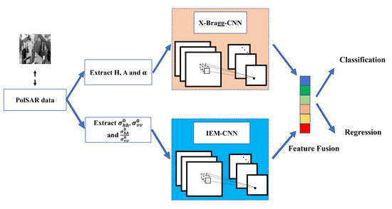
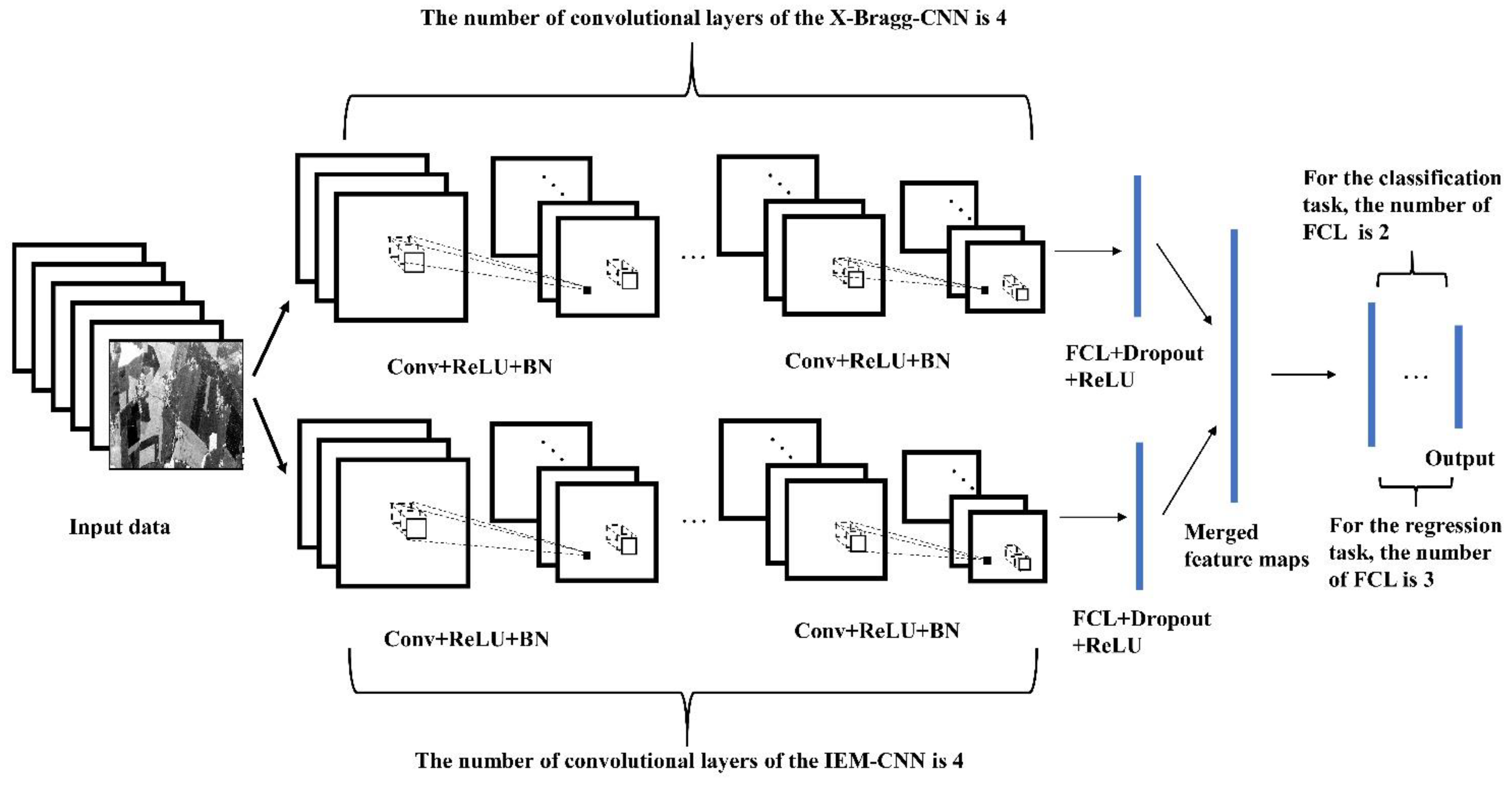
Generally, there are two strategies to invert the models. In the first strategy, according to the complexity of the model, the equation between known parameters and soil moisture can be solved by an analytical or numerical method. In the second strategy, a complex network is generated based on training. A network, such as MLP and CNN, can represent the complex nonlinear relationship between known parameters and soil moisture. Because the X-Bragg model and IEM are too complex, it is almost impossible to get the equation analytically using the two models’ parameters. Therefore, this paper attempts to use the CNN combined with the physical model to solve the problem of soil moisture inversion. At present, whether it is classification or parameter inversion, most CNNs are trained directly with original data or image data. However, this requires a large amount of data to adjust the model parameters. A priori knowledge, e.g., about functional expressions of mappings or about serviceable parameters, can be provided by the physical model. So we can relax the data requirements by combining the physical models. Meanwhile, the CNN can use the spatial information to automatically learn the features of the given data by a convolution kernel, which can solve the problem of low accuracy caused by physical models that have not been calibrated with real surface data. The dual-channel CNN is used to estimate soil moisture from a simulated dataset and real bare surface data. The experimental results shows that the dual-channel CNN extracts the features of the two model parameters and incorporates their strengths. Compared with other inversion methods, the main contributions of this method are as follows:

• Based on two scattering models, namely the X-Bragg model and the IEM, we make full use of the amplitude and phase information of PolSAR data, which can expand the applicable range of roughness and improve the inversion accuracy.
• The dual-channel convolutional neural network, which makes full use of spatial information and adds a dropout layer to reduce the overfitting, is used to perform the feature fusion of the parameters extracted from the scattering model.
• We use the dual-channel convolutional neural network to design a framework, which can perform coarse-grained qualitative classification and fine-grained quantitative regression to suit different tasks.

The remainder of this paper is organized as follows. Section 2 introduces the proposed method of this paper. In Section 3, we introduce the dataset. Experimental results and discussion are given in Section 4. Section 5 provides the main conclusions.

2. Methods

The overall flowchart of our proposed method is shown in Figure 1. Two classic physical scattering models are chosen to generate simulated data and extract the parameters, which are the X-Bragg model and the IEM. The potential of the proposed method in soil moisture inversion is verified by simulated data, which is represented by the dark blue arrow in Figure 1. Then we use the field data to verify the performance of the proposed method, which is represented by the light blue arrow in Figure 1. The X-Bragg model is a soil surface parameter inversion algorithm based on the full polarization SAR data. It uses the amplitude and phase information of the full polarization SAR data and separates the estimation of roughness from the estimation of soil moisture to improve the inversion accuracy. However, in the X-Bragg model, the roughness scope is not very wide (ks ≤ 1), so we choose to combine the X-Bragg model with the IEM. The IEM is a classic physical model with a wide range of roughness adaptation. The accuracy of inversion can be greatly improved by using two classical models for feature fusion. In this paper, we use the dual-channel CNN to perform feature fusion on the two models. The first channel is used to extract the features of three parameters within the X-Bragg model (X-Bragg-CNN), and the second channel is used to extract the features of three parameters within the IEM (IEM-CNN). The dual-channel features are fused in the fully connected layer (FCL) to estimate the soil moisture. Since the physical model inversion obtains the relationship between the backscatter coefficients and soil moisture by establishing an idealized model of the surface. This relationship has not been calibrated with real surface data. However, the CNN solves the problem of the physical model by extracting features from real surface data through supervised learning. For bare soil, due to the influence of irrigation methods, we can assume that soil moisture is approximate within a certain spatial neighborhood. Therefore, the CNN can obtain more spatial features such as the distribution and change of roughness and spatial variation characteristics around the target pixel than MLP by extracting local patches composed of the central pixel and surrounding pixels. In this paper, the CNN can achieve higher accuracy than MLP under the same training sample. Therefore, our method can accurately and efficiently perform soil moisture inversion. We design a framework based on the dual-channel CNN, which includes a coarse-grained classification network and a fine-grained regression network. Through this framework, the soil moisture inversion can be effectively performed within different situations. For example, we can use the classification network to classify the range of soil moisture or use the regression network to make accurate predictions of soil moisture. This section introduces the specific details of the main steps.

2.1. Extraction of H, A, and α by the X-Bragg Model

To obtain the polarization parameters of different values of soil moisture with full polarimetric SAR data, the X-Bragg model is used to simulate the coherence matrix of the L-band (1.3GHz) with a surface roughness (ks ≤ 1.5). However, the effective range of the roughness of the X-Bragg model is ks ≤ 1. Allain et al. [31] showed that the roughness range of the IEM simulated data can be extended to ks ≤ 1.5, so the X-Bragg model is modified to expand its applicable roughness. Reference [31] shows that the surface roughness has an approximate linear relationship with anisotropy within the range of ks ≤ 1.5 based on the L-band data simulated by the IEM. Therefore, we can modify the X-Bragg model to extend its roughness application range. Specifically, the polarization scattering matrix of the rough Bragg surface completely describes its polarization backscattering behavior, which can be written as

$$[\mathrm{S}] = \left[\begin{array}{cc}{S}_{HH}& S_{HV}\\ S_{VH}& S_{VV}\end{array}\right] = m_s\left[\begin{array}{cc}{R}_S& 0\\ 0& R_P\end{array}\right]$$

(1)

where $m_s$ is the backscattering amplitude containing surface roughness information, and $R_P$ and $R_S$ are defined as Equations (2) and (3). $R_P$ is the Fresnel reflection coefficient of vertical polarization and is given by

$$R_p = \frac{({\epsilon }_r-1)\{{\sin }^2\theta -{\epsilon }_r(1+{\sin }^2\theta )\}}{{({\epsilon }_r\cos \theta +\sqrt{{\epsilon }_r-{\sin }^2\theta })}^2}$$

(2)

$R_S$ is the Fresnel reflection coefficient of horizontal polarization and is given by

$$R_S = \frac{\cos \theta -\sqrt{{\epsilon }_r-{\sin }^2\theta }}{\cos \theta +\sqrt{{\epsilon }_r-{\sin }^2\theta }}$$

(3)

${\epsilon }_r$ is the dielectric constant. When we replace the scattering vector with the scattering amplitude and the Bragg scattering coefficient, the scattering vector $\overrightarrow{k}$ and the Bragg coherence matrix [T] are defined as Equations (4) and (5).

$$\overrightarrow{k} = m_s[\begin{array}{ccc}{R}_S+R_P& R_S-R_P& 0{]}^T\end{array}$$

(4)

$$[\mathrm{T}] = {\overrightarrow{\mathrm{kk}}}^{\ast } = m_s{}^2\left[\begin{array}{ccc}{\left|R_S+R_p\right|}^2& \left(R_S+R_P\right){\left(R_S-R_P\right)}^{\ast }& 0\\ \left(R_S-R_P\right){\left(R_S+R_P\right)}^{\ast }& {\left|R_S-R_P\right|}^2& 0\\ 0& 0& 0\end{array}\right]$$

(5)

For the sake of introducing roughness disturbance, the surface is modeled as a reflection symmetric depolarizer by rotating the Bragg coherency matrix with an angle β [32] as shown in Equation (6).

$$[\mathrm{T}(\beta )] = \left[\begin{array}{ccc}1& 0& 0\\ 0& \cos 2\beta & \sin 2\beta \\ 0& -\sin 2\beta & \cos 2\beta \end{array}\right]\left[\begin{array}{ccc}{\left|R_S+R_P\right|}^2& \left(R_S+R_P\right){\left(R_S-R_P\right)}^{\ast }& 0\\ \left(R_S-R_P\right){\left(R_S+R_P\right)}^{\ast }& {\left|R_S-R_P\right|}^2& 0\\ 0& 0& 0\end{array}\right]\left[\begin{array}{ccc}1& 0& 0\\ 0& \cos 2\beta & \sin 2\beta \\ 0& -\sin 2\beta & \cos 2\beta \end{array}\right]$$

(6)

Then, a configurational averaging is performed over a given distribution P (β) of β.

$$[\mathrm{T}] = {\int }_0^{2\pi }[T(\beta )]P(\beta )d(\beta )$$

(7)

The width of the assumed distribution corresponds to the amount of roughness disturbance of the modeled surface. We assume P (β) to be a uniform distribution with width ${\beta }_1$, such as

$$\mathrm{P}(\beta ) = \{\frac{1}{2{\beta }_1}|\beta |\le {\beta }_1, 0\le {\beta }_1\le \frac{\pi }{2}$$

(8)

Therefore, the coherence matrix of a rough surface is defined as Equation (9). The coefficients C1, C2, and C3 describing the coherence matrix are given by Equation (10).

$$[\mathrm{T}] = \left[\begin{array}{ccc}{T}_{11}& T_{12}& T_{13}\\ T_{21}& T_{22}& T_{23}\\ T_{31}& T_{32}& T_{33}\end{array}\right] = \left[\begin{array}{ccc}C1& C2\sin c\left(2{\beta }_1\right)& 0\\ C2sinc\left(2{\beta }_1\right)& C3\left(1+\sin c\left(4{\beta }_1\right)\right)& 0\\ 0& 0& C3\left(1-sinc\left(4{\beta }_1\right)\right)\end{array}\right]$$

(9)

$$C1 = {\left|R_S+R_P\right|}^2, C2 = \left(R_S+R_P\right)\left(R_S{}^{\ast }-R_P{}^{\ast }\right), C3 = {\left|R_S-R_P\right|}^2/2$$

(10)

The X-Bragg model uses the parameter ${\beta }_1$ to describe the surface roughness. We use the incident angle, dielectric constant, and ${\beta }_1$ to simulate the coherence matrix T of the rough surface. Reference [23] shows that the relationship between ks, A, and ${\beta }_1$, which is given by

$$ks = 1-\mathrm{A}, 0\le \mathrm{A}\le 1$$

(11)

$$\mathrm{A} = 1-\frac{1}{90}\times {\beta }_1, 0\le {\beta }_1\le \frac{\pi }{2}$$

(12)

We can obtain the relationship between ks and ${\beta }_1$ through Equations (11) and (12).

$$ks = \frac{1}{90}\times {\beta }_1, 0\le {\beta }_1\le \frac{\pi }{2}$$

(13)

Here, we modify the X-Bragg model to expand the applicable range of roughness ks from 1.0 to 1.5. We know from reference [31] that the surface roughness has an approximate linear relationship with the anisotropy within the range of ks ≤ 1.5 based on the L-band data simulated by the IEM, which is given by

$$ks = 1.5\times (1-\mathrm{A}), 0\le \mathrm{A}\le 1$$

(14)

By combining Equations (12) and (14), we can obtain the modified equation between ks and ${\beta }_1$.

$$ks = \frac{1}{60}\times {\beta }_1, 0\le {\beta }_1\le \frac{\pi }{2}$$

(15)

The simulated T matrix uses the H/A/α decomposition method proposed by Cloude and Pottier [33] to extract feature parameters.

$$\mathrm{T} = \sum _{i=1}^3{\lambda }_i{u}_i{u}_i^H$$

(16)

where

$$u_i = e^{j{\varphi }_i}{\left[\cos {\alpha }_i\sin {\alpha }_i\cos {\beta }_i{e}^{j{\delta }_i}\sin {\alpha }_i\cos {\beta }_i{e}^{j{\gamma }_i}\right]}^T$$

(17)

${\alpha }_i$ is the target scattering mechanism and ${\lambda }_i$ is the eigenvalue of matrix T. Three important physical features can be obtained through the H/A/α decomposition of the T matrix. We normalize the eigenvalues by the absolute scattering amplitude to get the scattering probability $p_i$, which is given by

$$p_i = \frac{{\lambda }_i}{{\displaystyle \sum _{j=1}^3}{\lambda }_j}\to p_1+p_2+p_3 = 1$$

(18)

We can obtain H and A by using the probability $p_i$, defined as

$$\mathrm{H} = -\sum _{i=1}^3{p}_i{\log }_3{p}_i$$

(19)

$$\mathrm{A} = \frac{p_2-p_3}{p_2+p_3}$$

(20)

The third important parameter can be obtained by eigenvectors, and α can be calculated by the target scattering mechanism ${\alpha }_i$, which is defined as

$$\alpha = \sum _{i=1}^3{P}_i{\alpha }_i$$

(21)

We use the X-Bragg model to simulate the T matrix of the rough surface and extract H, A, and α using the H/A/α decomposition method.

2.2. Extraction of ${\sigma }_{hh}^0$,${\sigma }_{vv}^0$, and ${\sigma }_{hh}^0/{\sigma }_{vv}^0$ by the IEM

To make up for the problem that the roughness of the X-Bragg model is not suitable for a wide range, we choose the IEM to simulate the backscattering coefficient of the L-band (1.3 GHz) with a surface roughness (ks ≤ 1.5). Under medium and small roughness, the single scattering form of the IEM is denoted as

$${\sigma }_{qp}^o = \frac{k^2}{2}\exp \left(-2s^2{k}_z^2\right)\sum _{n=1}^{\infty }{s}^{2n}{|I_{qp}^n|}^2\frac{W^{\left(n\right)}(-2k_x, 0)}{n_{!}}$$

(22)

where $k_z = kcos\theta$, $k_x = ksin\theta$, θ is the incident angle, and $p,q = h,v$.

$$I_{qp}^n = {\left(2k_z\right)}^n{f}_{qp}\exp \left(-s^2{k}_z^2\right)+\frac{k_z^n\left[F_{qp}\left(-k_x,0\right)+F_{qp}\left(k_x,0\right)\right]}{2}$$

(23)

$$f_{vv} = \frac{2R_P}{\cos \theta },f_{hh} = -\frac{2R_S}{\cos \theta }$$

(24)

$$F_{vv}\left(-k_v,0\right)+F_{vv}\left(k_x,0\right) = \frac{2{\sin }^2\theta {\left(1+R_p\right)}^2}{\cos \theta }\times \left[\left(1-\frac{1}{{\epsilon }_r}\right)+\frac{{\mu }_r{\epsilon }_r-{\sin }^2\theta -{\epsilon }_r{\cos }^2\theta }{{\epsilon }_r^2{\cos }^2\theta }\right]$$

(25)

$$F_{hh}\left(-k_x,0\right)+F_{hh}\left(k_x,0\right) = -\frac{2{\sin }^2\theta {\left(1+R_S\right)}^2}{\cos \theta }\times \left[\frac{{\epsilon }_r-{\sin }^2\theta -{\cos }^2\theta }{{\cos }^2\theta }\right]$$

(26)

$R_P$ and $R_S$ are shown in Equations (2) and (3), respectively.${\epsilon }_r$ is the dielectric constant.$W^{\left(n\right)}$ is the Fourier transform of the nth power of the surface correlation coefficient.

$$W^{(n)}=\frac{l^2}{n^2}{\left[1+4{\left(\frac{\mathrm{klsin}\theta }{n}\right)}^2\right]}^{-1.5}$$

(27)

where $l$ is the correlation length.

We generate the backscatter coefficients of the HH polarization (${\mathsf{\sigma }}_{hh}^0$) and VV polarization (${\mathsf{\sigma }}_{vv}^0$) through the IEM and calculate the co-polarization ratio (${\mathsf{\sigma }}_{hh}^0/{\mathsf{\sigma }}_{vv}^0$).

2.3. Design of the Dual-Channel Convolutional Neural Network

A typical convolutional neural network is generally composed of a convolutional layer, a pooling layer, and an FCL. Through this cascading structure, high-level features can be learned from raw data for classification and regression. The structure of the dual-channel CNN used in this paper is shown in Figure 2. The entire network structure can be divided into two parts: feature extraction and output prediction. In the feature extraction part, the first channel (X-Bragg-CNN) is used to extract the features of three parameters within the X-Bragg model, and the second channel (IEM-CNN) is used to extract the features of three parameters within the IEM. Four convolutional layers and one FCL are used in the X-Bragg-CNN, while the IEM-CNN also uses four convolutional layers and one fully connected layer. The convolutional layers include the functions of convolution, rectified linear unit (ReLU), batch normalization (BN) [34], and dropout [35]. The role of the BN layer is to solve the gradient disappearance and the gradient explosion while speeding up the network learning rate. The function of the dropout layer is to let a certain neuron stop working with probability p when we feed-forward propagation so that the model can reduce overfitting and have stronger generalization. The features extracted by the dual channels are fused in the fully connected layer. The classification network and the regression network only differ in the output prediction. The output layer of the classification network is a classifier composed of two fully connected layers, and the output layer of the regression network is a regressor composed of three fully connected layers. The configuration of the dual-channel classification CNN is shown in

Table 2. Configuration of the classification CNN.

Type	Dual-Channel CNN
	X-Bragg-CNN	IEM-CNN
Convolution layer	8@3 × 3/1/0	8@3 × 3/1/0
Convolution layer	16@3 × 3/1/0	16@3 × 3/1/0
Convolution layer	24@3 × 3/1/0	24@3 × 3/1/0
Convolution layer	32@3 × 3/1/0	32@3 × 3/1/0
Fully connected layer	120	120
Merge layer	240
Fully connected layer	84
Fully connected layer	C (Class number) In this paper, C of the simulated dataset is 8, and the field dataset is 5
Dropout (ratio:0.5)

.

Table 3. Configuration of the regression CNN.

Type	Dual-Channel CNN
	X-Bragg-CNN	IEM-CNN
Convolution layer	8@3 × 3/1/0	8@3 × 3/1/0
Convolution layer	16@3 × 3/1/0	16@3 × 3/1/0
Convolution layer	24@3 × 3/1/0	24@3 × 3/1/0
Convolution layer	32@3 × 3/1/0	32@3 × 3/1/0
Fully connected layer	120	120
Merge layer	240
Fully connected layer	84
Fully connected layer	32
Fully connected layer	1
Dropout (ratio:0.5)

shows the configuration of the dual-channel regression CNN. Next, we will describe the details of the CNN.

The input data is an 11 $\times$ 11 $\times$ 6 multi-dimensional matrix, which indicates that the local patch size is 11 $\times$ 11 and the number of input feature channels is 6. In the convolutional layer, the input data I and a set of preset filters W are convolved and then added to the offset b. Finally, the nonlinear activation function, as shown in Equation (28), is used to obtain the local feature F.

$$F_{i^{\prime },j^{\prime }} = f(b_{k^{\prime }}+\sum _{i=1}^m\sum _{j=1}^n{W}_{ij{k}^{\prime }}{I}_{i^{\prime }+i,j^{\prime }+j})$$

(28)

where f (⋅) is ReLU. The ReLU function can avoid gradient dissipation and reduce the training time, which is defined as

$$\mathrm{f}\left(x_{ij}\right) = \max \left\{0,x_{ij}\right\}$$

(29)

In this paper, for the X-Bragg-CNN, the input data size is 11 × 11 × 3. The first convolutional layer size is set to 3 × 3 with a stride of 1 pixel. After the first convolutional layer, we can get 8 feature maps with a size of 9 × 9. The second convolutional layer size is set to 3 × 3 with a stride of 1 pixel. After the second convolutional layer, we can get 16 feature maps with a size of 7 × 7. The third convolutional layer size is set to 3 × 3 with a stride of 1 pixel. After the third convolutional layer, we can get 24 feature maps with a size of 5 × 5. The fourth convolutional layer size is set to 3 × 3 with a stride of 1 pixel. After the fourth convolutional layer, we can get 32 feature maps with a size of 3 × 3. The IEM-CNN has the same configuration structure as X-Bragg-CNN.

The fully connected layer maps the feature map to the sample label space, which can greatly reduce the impact of feature location. For the X-Bragg-CNN, 32 feature maps with a size of 3 × 3 are transformed into a one-dimensional vector with 120 neurons through a fully connected layer. For the IEM-CNN, 32 feature maps with a size of 3 × 3 are also transformed into a one-dimensional vector with 120 neurons through a fully connected layer. By connecting two one-dimensional vectors, we can get a one-dimensional feature vector with 240 neurons. We put the obtained one-dimensional vector into a fully connected layer to obtain a one-dimensional vector with 84 neurons. When we perform classification tasks, the output is put into a fully connected layer, which outputs a vector with C neurons, where C is the number of categories. When we perform the regression task, the output is put into two fully connected layers; the first connected layer outputs a vector with 32 neurons, and the second connected layer outputs our regression value.

2.4. Data Preprocess and Training

To use the CNN for soil moisture inversion, we need to preprocess the data so that it can be used as the input of the network. The CNN not only use pixel values but also use spatial patterns to extract features. Thus, each pixel is represented by a local patch with a size of 11 × 11. We use a 11 × 11 sliding window to slide pixel by pixel in the extracted six polarization parameter matrices to generate samples with a size of 11 × 11 × 6.

During the training, the model’s hyperparameters are determined by a fivefold cross-validation method. We divide the training dataset into five mutex subsets of the same size and keep the data category distribution in each subset consistent. Four subsets are used for training at a time, and the remaining subset is used for validation to adjust the hyperparameters. Five sessions of training and validation are conducted to ensure that all data are trained. By training datasets and verifying them, we train 50 epochs at a time and fine-tune the network layer number and hyperparameters until the network can fit better results. We use the Adam optimization algorithm [36]. Each batch size has 128 samples, and the initial learning rate is set to 0.001. This algorithm optimizes the random objective function based on a step degree through low-order adaptive moment estimation. It is computationally efficient and has a small memory requirement. Usually, the learning rate can be automatically adjusted without adjusting the hyperparameters. In the dual-channel CNN, we set the dropout ratio to 0.5 and use it behind the FCL. In the network, the part with more parameters is easy to overfit. The function of the convolutional layer is to extract features, and adjacent pixels in the convolutional layer share much of the same information. If any of them are inactivated, the information they contain may be passed from the adjacent pixels that are still active. In the model, the fully connected layer contains most of the network parameters and is not affected by the feature location. So we use dropout after the fully connected layer. Meanwhile, we set the dropout ratio to 0.5 to maximize the randomly generated network structure so as to reduce overfitting.

3. Datasets

This paper uses two datasets. The first is a simulated dataset, which is generated using the X-Bragg model and the IEM to test the feasibility of the proposed method. The second is the field dataset, used to verify the effectiveness of the actual soil moisture inversion.

3.1. Simulated Dataset

To test the performance of soil moisture inversion using convolutional neural networks, the most important step is to obtain the data covering a wide range of soil moisture. However, it is difficult for us to build a complete soil moisture dataset, which requires a large number of field measurements. Therefore, we use two backscatter models to simulate SAR radar signals for different soil surface parameters. The backscatter models selected in this paper are the X-Bragg model and the IEM. In the Section 2, we introduce the principles of the X-Bragg model and the IEM. Next, we describe the details of the specific step for generating simulated data.

We simulate the T matrix, which gives soil moisture and roughness by using Equations (2), (3), (9), (10), and (15). After obtaining the T matrix, we extract the polarization parameters by H/A/α decomposition from the T matrix using Equations (16) and (18–21). Then, we simulate the backscattering coefficients (${\mathsf{\sigma }}_{hh}^0$ and ${\mathsf{\sigma }}_{vv}^0$) of same moisture and roughness by using Equations (22)–(27) and calculate the co-polarization ratio (${\mathsf{\sigma }}_{hh}^0/{\mathsf{\sigma }}_{vv}^0$).

It can be concluded from reference [23] that the effective range of soil moisture in the X-Bragg model is 0–35%. When the soil moisture exceeds 35%, the inversion performance decreases obviously. The soil moisture range is set slightly above 35% to observe the inversion performance of the proposed method in the simulated dataset. Therefore, we consider 8 soil moisture values (mv between 3% and 38% with a step of 5%), 100 surface roughness values (ks between 0.015 and 1.5 with a step of 0.015), and 2 incident angles, which are 35° and 45°. We apply the 45° incident angle to simulate data with the moisture value of 3–18% and the 35° incident angle to simulate data with the moisture value of 23–38%. To expand the number of samples at each moisture level, a small neighboring range of central values will also be considered as the same category. For example, 2.5–3.5% of water content will be classified into the 3% moisture category. In our experiment, the small neighboring range is set to (mv − 0.5%, mv + 0.5%), at the intervals of 0.01%. In this way, we can generate 10,000 samples for each soil moisture value, and a total of 80,000 samples. To use the spatial information, the 10,000 samples of each moisture value are placed in a 100 by 100 matrix. The elements in each row of each matrix have the same soil moisture value but different roughness values, while the elements in each column have the same soil roughness but different soil moisture values. This placement method can approximate the fluctuation of soil surface roughness. The generated simulated data’s ground truth is shown in Figure 3.

3.2. Field Dataset

The field dataset is the surface measurement data of the Gömin farm in the DEMMIN area within northern Germany obtained during the AgriSAR campaign in 2006 [37]. The data used in our experiment are four fully polarimetric ESAR images (L-band) obtained on 19 and 20 April 2006. The soil moisture truth values used in this paper are measured on site by the ISSIA, LHWM, and LMU teams using TDR with a depth of 5 cm, and their average values are calculated. Among them, 45 samples are measured in the E1 region, 80 in the E2 region, 90 in the E3 region, 45 in the E4 region, and 30 in the E5 region. The E-SAR data can be radiated through the PolSARpro toolbox developed by ESA to obtain the${\sigma }_{hh}^0$, ${\sigma }_{vv}^0$, H, A, and α. The dataset contains five different soil moisture values, which are divided into five categories. As shown in Figure 4, we use the polygons to label areas with known soil moisture. Assuming that the soil moisture in the same area is equal to the average value calculated after measuring different points with a TDR. The specific soil moisture and regional labels are shown in

Table 4. Soil moisture data table.

Filed ID	Date	Average Soil Moisture (%)
E1	19-Apr-06	20.1
E2	19-Apr-06	23
E3	19-Apr-06	24.3
E4	19-Apr-06	26.8
E5	20-Apr-06	13.8

.

4. Experiments and Discussion

In this experiment, we conduct experiments on both simulated data and field data. Then, we discuss the influence of different patch sizes on the inversion results, and the feature maps extracted by the CNN are visualized and analyzed.

4.1. Simulated Data

In the Section 3, we generate 80,000 samples corresponding to 8 soil moisture values. Each sample includes ${\mathsf{\sigma }}_{hh}^0$, ${\mathsf{\sigma }}_{vv}^0$,${ \mathsf{\sigma }}_{hh}^0/{\mathsf{\sigma }}_{vv}^0$, H, A, and $\alpha$. As an example, the scattering entropy of two samples with 3% and 18% true moisture values are shown in Figure 5. It can be seen from Figure 5 that for different soil moistures, their scattering entropy is quite different. It is precisely because of the obvious difference in the scattering entropy that the CNN can identify and estimate different soil moisture values after the necessary training process. Because roughness and soil moisture change regularly in the matrix, Figure 5 appears to be regular. Meanwhile, because the roughness and soil moisture are not exactly the same at each point, we can see that the scattering entropy fluctuates in a small range.

We use an 11 $\times$ 11 sliding window to generate 10,000 samples for each soil moisture data, so for 8 moisture values, we generate a total of 80,000 samples. We randomly select 1% of samples in each category for training, and adopt the fivefold cross-validation method to determine the hyperparameters. After determining the hyperparameters, we train all the training samples for 50 epochs to get the final model. The remaining 99% of the samples are tested to get the final classification accuracy. Then we use the same samples for training and randomly select five samples from each category test dataset to test the regression network. The selection of samples in this way can indicate that the method in this paper has the capability of extracting high-level semantic information from the given features using small amounts of data for soil moisture classification and regression.

In this paper, we use three indicators to analyze and discuss the experimental results. The inversion accuracy (IA) can be used to describe the accuracy of the classification, which is defined as Equation (30). The deviation between the predicted value and the true value can be expressed as RMSE, which is denoted as Equation (31). The determination coefficient ($r^2$), given by Equations (32)–(34), is an indicator to judge the fitting degree of the model. The larger the determination coefficient, the better the model fitting is.

• Inversion accuracy (IA) and average IA

  $$\mathrm{IA}(\%) = \frac{{\displaystyle \sum _{i=1}^K}I\{y_{Classification}^i=y_{real}^i\}}{K}\ast 100\%$$

  (30)

  $$\mathrm{Average} \mathrm{IA}(\%) = \frac{{\displaystyle \sum _{i=1}^N}I\{y_{Classification}^i=y_{real}^i\}}{N}\ast 100\%$$

  (31)
• Root mean square error (RMSE)

  $$\mathrm{RMSE} = \sqrt{\frac{1}{N}\sum _{i=1}^N{(y_{Regressiom}^i-y_{real}^i)}^2}$$

  (32)
• Coefficient of determination (${\mathrm{r}}^2$)

  $$\mathit{SST} = \sum _{i=1}^N{(y_{real}^i-{\bar{y}}_{real}^i)}^2$$

  (33)

  $$\mathit{SSE} = \sum _{i=1}^N{(y_{Regressiom}^i-y_{real}^i)}^2$$

  (34)

$$r^2 = 1-\frac{SSE}{SST}$$

(35)

where K is the number of test samples for each type of soil moisture, N is the total number of test samples, $y_{Classification}$ is the classification network output value, $y_{Regression}$ is the regression network output value, $y_{real}$ is the true value of soil moisture, and ${\overline{y}}_{real}$ is the average value of the true value of soil moisture. For the classification network, we choose the IA to evaluate the performance of the network, and for the regression network, we choose the RMSE and $r^2$ to analyze the experimental results. For the sake of considering the finite radiometric resolution of SAR data, we add different levels of multiplicative noise to the simulated data. The data after adding the multiplicative noise model is defined as

$$y(k,l) = x(k,l)+x(k,1)v(k,l)$$

(36)

where y(k,l) is the intensity or amplitude of the (k,l) pixel after adding noise in the simulated data, x(k,l) is the intensity or amplitude of the (k,l) pixel before adding noise in simulated data, and v(k,l) is noise. In this paper, the noise obeys the Gaussian distribution with a mean of zero and a standard deviation of ${\mathsf{\sigma }}_{\mathrm{v}}$. The ratio of standard deviation to mean value can effectively measure the noise of SAR image. Thus, we introduce the equivalent number of looks (ENL) [38], which is defined as

$$\beta = \frac{\delta }{<x>}$$

(37)

$$\mathrm{ENL}(\mathrm{I}) = \frac{1}{{\beta }^2}$$

(38)

where $\mathsf{\delta }$ is the standard deviation of the SAR images and <x> is the mean value of the SAR images. We calculate the ENL of the original simulated data, and the result is 4.5-look. Then we add noise to the diagonal of T matrix and backscattering coefficient matrix of the simulated data and adjust the standard deviation of noise. We judge the degree of adding noise by calculating the ENL. We add three levels of noise to the simulated data. After adding noise, the ENL of simulated data are the 4-look, 3-look, and 2-look. We use the same hyperparameters and the sample in the same place to train and predict the original simulated data with different levels of noise and analyze the statistical results.

The results are given in

Table 5. Simulated data average IA and IA of dual-channel CNN in different levels of noise.

ENL	Average IA	3%	8%	13%	18%	23%	28%	33%	38%
4.5-look	97.96%	100%	99.80%	98.87%	98.74%	99.54%	97.63%	95.22%	93.89%
4-look	96.05%	99.95%	99.02%	99.15%	98.42%	98.65%	94.46%	91.77%	86.96%
3-look	92.56%	99.81%	98.68%	98.27%	97.02%	93.68%	87.20%	88.39%	77.42%
2-look	87.59%	98.97%	98.46%	97.91%	96.03%	89.20%	75.55%	75.51%	69.09%

and

Table 6. Simulated data RMSE and r² of the dual-channel CNN in different levels of noise.

ENL	RMSE (%)	r2
4.5-look	0.65	0.99
4-look	1.60	0.98
3-look	1.89	0.97
2-look	2.91	0.94

and Figure 6. The result shows that when no noise is added to the simulated data, the inversion accuracy can reach 97.96%. We can notice that when the moisture exceeds 30%, the accuracy rate decreases to a certain extent. The scope of the X-Bragg model is mv < 40%. When the moisture value is close to 40%, the saturation phenomenon occurs, showing that the polarization characteristics of the change are not obvious. Thus, there is a slight drop in the inversion accuracy. After adding the different levels of noise, the inversion accuracy decreases with the noise levels improvement. Due to the existence of saturation phenomenon, the accuracy is more affected by noise with an increase in the moisture value. When the ENL is higher than 2-look, the IA can be larger than 85%, and the determination coefficient is greater than 0.93. Based on the above phenomena, we can see that the proposed method has great potential in soil moisture inversion.

4.2. Field Data

Here, we prove the effectiveness of the method proposed in this paper by simulated datasets. The soil moisture is inverted through field data. Some emerging literature [39] suggests that randomly sampling data may make the training set and test data very close. In this regard, the training dataset and the test dataset do not exist independently, which have a certain spatial correlation. The inversion results may be improved by the high correlation. To avoid the effect of this high correlation and reduce the difficulty of collecting the truth value of soil moisture, the adaptability of different sampling strategies using field datasets under random sampling and spatially disjoint sampling are compared in this paper. We use different sampling strategies to select 500 sample points from each area for training, and the remaining sample points are used for testing. The black dots in Figure 7c,d are shown in the selection of training samples of random sampling and spatially disjoint sampling. The number of training samples and test samples is given in

Table 7. The number of training and test samples.

Field ID	The Number of Training Samples	The Number of Test Samples
E1	500	616,480
E2	500	120,282
E3	500	716,987
E4	500	344,954
E5	500	64,263

. The fivefold cross-validation method is adopted to determine the hyperparameters. After determining the hyperparameters, we train all the training samples for 50 epochs to get the final model. We use the classification models trained by different sample selection strategies to predict test data. As shown in

Table 8. Comparison between random sampling and spatially disjoint sampling on the field dataset.

Field ID	Random	Disjoint
E1 IA	97.61%	97.28%
E2 IA	99.68%	99.77%
E3 IA	95.81%	95.50%
E4 IA	95.08%	90.00%
E5 IA	98.18%	97.52%
Average IA	96.59%	95.39%

, we can see that the accuracy of spatially disjoint sampling is 1.2% lower than that of random sampling. For the spatially disjoint sampling method, the accuracy mainly decreases in E4 regions. This is because, as shown in the Pauli figure, the surface of the E4 region is not very smooth. When we use spatial disjoint sampling, we may not be able to learn all the characteristics of terrain changes. The correlation between train dataset and test dataset will be greatly reduced, which leads to a decrease in accuracy. However, the performance gap between random sampling and spatially disjoint sampling is acceptable. The classification result prediction map of the two sampling strategies is shown in Figure 7e,f. In the subsequent experiments of this paper, we use the samples obtained by the spatially disjoint sampling strategy to train the model.

To ensure that there is no overfitting of our model, as shown in Figure 8, we draw the curve of training accuracy and test accuracy, increasing with the number of epochs. The blue line represents the training accuracy curve, and the green line represents the test accuracy curve. We see from the curve that both the training accuracy and the test accuracy are rising gradually and tend to be stable after reaching 95%. Therefore, there is no overfitting in our model.

To verify the effectiveness of the network proposed in this paper, we conduct two sets of comparative experiments for both classification and regression network. For the coarse-grained classification network, we put the samples into the dual-channel CNN, MLP, and SVM for training. As shown in

Table 9. Classification result of the dual-channel CNN, MLP, and SVM.

Category	Dual-Channel CNN	MLP	SVM
E1 IA	97.28%	94.36%	94.62%
E2 IA	99.77%	97.96%	97.92%
E3 IA	95.50%	90.15%	89.63%
E4 IA	90.00%	79.74%	82.05%
E5 IA	97.52%	77.62%	85.88%
Average IA	95.39%	89.82%	90.33%
Testing time (s)	50	20	30

, the average inversion accuracy of the proposed model is 95.39%, which is 5.57% higher than that of the MLP and 5.06% higher than that of SVM. Compared with the MLP and SVM, when using the same parameters, our proposed method is better than the traditional neural network and the SVM because the convolutional neural network uses spatial information, which can get better classification results when using a small number of the same training samples.

In the second set of competitive experiments, we use three single-channel CNNs to train the model with the same hyperparameters and test the samples. They are X-Bragg-CNN, IEM-CNN, and 6CH-CNN, whose input features are directly concatenated without using dual channels. As shown in

Table 10. Classification result of the dual-channel CNN, X-Bragg-CNN, IEM-CNN, and 6CH-CNN.

Category	Dual-Channel CNN	X-Bragg-CNN	IEM-CNN	6CH-CNN
E1 IA	97.28%	88.99%	77.39%	96.52%
E2 IA	99.77%	97.10%	98.93%	99.09%
E3 IA	95.50%	83.68%	90.66%	92.50%
E4 AI	90.00%	89.86%	73.06%	86.06%
E5 IA	97.52%	94.89%	88.91%	97.14%
Average IA	95.39%	87.76%	83.42%	93.18%
Testing time (s)	50	31	31	35

, the average accuracy of a dual channel in the classification network is higher than that of a single channel. Different channels have very different accuracy rates for areas with different moistures, which shows that different areas have different main characteristics. We can see from the results that the accuracy in most areas of the IEM-CNN is lower than that of the X-Bragg-CNN. This is because the X-Bragg-CNN makes full use of the amplitude and phase information of the full polarization SAR data and takes the anisotropy as one of the features of the network input to complete the decoupling of soil moisture and roughness at the data level. The accuracy of the 6CH-CNN in the E4 region is lower than that of the X-Bragg-CNN. It can be seen from this that the direct connection of features will cause mutual interference between features. However, our proposed dual-channel CNN can independently extract advanced features of different parameters to improve the inversion accuracy.

For the fine-grained regression network, we use the same samples as classification network for training and all pixels for regression network test and indicator calculation. The predicted soil moisture maps are shown in Figure 9. As shown in Figure 9b, the soil moisture predicted by the dual-channel CNN correspond well with the soil moisture measured in-situ. For X-Bragg-CNN and IEM-CNN, the relationship between soil moisture and input parameters cannot be well fitted due to too few training samples and insufficient number of features. The RMSE and r² are given in

Table 11. Field data RMSE and r² of the dual-channel CNN, MLP, SVM, X-Bragg-CNN, IEM-CNN, and 6CH-CNN.

Net	RMSE (%)	r2
Dual-channel CNN	0.98	0.88
MLP	2.14	0.44
SVM	2.02	0.50
X-Bragg-CNN	1.82	0.59
IEM-CNN	2.32	0.40
6CH-CNN	1.37	0.77

. We can see from Table 11 that the dual-channel CNN has a lower RMSE and higher coefficient of determination than other methods, which means that the dual-channel CNN has higher inversion performance. The dual-channel CNN can make full use of spatial information and reduce mutual interference between features by using dual channels. Compared with the traditional neural network and convolutional neural network, the dual-channel CNN can reduce the RMSE by about 0.39–1.34% and increase r² by about 0.11–0.48. We verify the effectiveness of the proposed method by using L-band airborne data. It has weak penetration for C-band data. However, since this paper focuses on the bare soil region and there is no interference from vegetation, we consider that this method can also be applied to the C-band satellite data for soil moisture inversion of bare soil.

4.3. Different Size Patches and Visualization of Feature Maps

When we use the convolutional neural network, we take the patch composed of the center pixel and its neighborhood as the network input. Meanwhile, we serve the category of the center pixel as the label. The size selection of the patch should be related to the size of the target. If the patch size is too small, the CNN learns inadequate feature information which causes the low accuracy. However, if the patch size is too large, the network learns the redundant features. Not only will it increase the running time, but the accuracy is not significantly improved. To evaluate the influence of patch size on classification accuracy and running time, we perform the experiment with patch of 7 × 7, 11 × 11 and 15 × 15. We train and test on NVIDIA’s GeForce GTX 1060 with 6GB of GPU memory. As shown in

Table 12. Classification accuracy and running time for different patch sizes.

Patch Size	Average IA	Testing Time (s)
7 $\times$ 7	93.16%	45
11 $\times$ 11	95.39%	50
15 $\times$ 15	95.65%	65

, the classification accuracy when using the patch of 7 × 7 is lower than when using the patch of 11 × 11 and 15 × 15. If the size of the patch is too small, the convolutional neural network cannot extract adequate features. The classification accuracy when using the patch of 11 × 11 is almost the same as when using patch of 15 × 15. However, with almost the same accuracy, the running time when using the patch of 11 × 11 is shorter than when using the patch of 15 × 15. Therefore, we choose 11 × 11 as the patch size in our experiment.

To better represent the proposed dual-channel CNN model, we visualize the X-Bragg-CNN and the IEM-CNN. The visualization process of the dual channels is located in the first convolutional layer and the last convolutional layer. The visualization content includes input data visualization and feature extraction visualization. For input data visualization, two slices of 11 $\times$ 11 $\times$ 3, which come from the sample of the test dataset, are selected as an example to show the visualization process. We use the two slices as the X-Bragg-CNN input and the IEM-CNN input, respectively. Figure 10a,b shows the visualized images of the X-Bragg-CNN input and the IEM-CNN input, respectively. Since the X-Bragg-CNN input is significantly different from the IEM-CNN input, it is difficult to infer that the two inputs represent the same category through the input visual images. However, the obvious differences between the two input data represent different polarization characteristics of the same category. We extract these features separately through the dual-channel convolutional neural network and merge them to improve the inversion accuracy. After visualizing the input data, we put the data into the trained dual-channel CNN model for the visualization of extracting features. Figure 10c describes the visualization of extracting features using X-Bragg-CNN after the first convolution operation and ReLU operation. In the first round of feature extraction, the 11 $\times$ 11 $\times$ 3 X-Bragg-CNN input is processed by the 3 $\times$ 3 convolution kernel and is transformed into a 9 $\times$ 9 feature map as the output. Figure 10c shows three representative visualized images in the obtained feature map. It can be seen from the Figure 10c that many polarization features are extracted by convolution operation. Then, after the ReLU operation, some of them are set to 0. Figure 10d describes the visual process of feature extraction for the IEM-CNN input. It shows that the IEM-CNN can extract obvious features through a convolution kernel. We can see from the visualization of X-Bragg-CNN and IEM-CNN that we extract features of different polarization parameters to obtain different features. After feature fusion, we can use more features than one channel to enhance the inversion accuracy. The visual feature extraction process can help us check whether the dual-channel CNN is effectively trained and tell us how to extract features.

5. Conclusions

In this paper, we propose a dual-channel convolutional neural network based on polarimetric scattering models for soil moisture inversion and use this model to design a framework for soil moisture inversion in the bare land. The model puts The model puts H, A, α, ${\sigma }_{hh}^0$, ${\sigma }_{vv}^0$ and ${\sigma }_{hh}^0/{\sigma }_{vv}^0$ into different channels to extract features. Finally, the model after the feature fusion is used to invert the soil moisture. Experiments show that the dual-channel convolutional neural network model has a high precision inversion accuracy. In the classification network of qualitative analysis, the average inversion accuracy reaches 95.39%, and in the regression network of quantitative analysis, the r² and RMSE are 0.88 and 0.98% respectively. The above statistical results are superior to one-channel convolutional neural network and MLP, which indicates that the proposed method can be accurately applied to soil moisture inversion task in bare soil regions. The dual-channel CNN makes full use of spatial information and merges the information between different polarization parameters. A small number of samples can be used to get high inversion accuracy. Due to the physical models used in this paper are only applicable to bare soil and sparse vegetation cover areas, the effect of vegetation is not taken into account. In the future, we plan to combine the dual-channel convolutional neural network with the inversion model suitable for vegetation covered area for soil moisture inversion task in vegetation-covered areas.

References

1. King, C.; Baghdadi, N.; Lecomte, V.; Cerdan, O. The application of remote-sensing data to monitoring and modelling of soil erosion. Catena 2005, 62, 79–93. [Google Scholar] [CrossRef]
2. Bronstert, A.; Creutzfeldt, B.; Gräff, T.; Hajnsek, I.; Heistermann, M.; Itzerott, S.; Jagdhuber, T.; Kneis, D.; Lück, E.; Reusser, D.E.; et al. Potentials and constraints of different types of soil moisture observations for flood simulations in headwater catchments. Nat. Hazards 2012, 60, 879–914. [Google Scholar] [CrossRef]
3. Berthet, L.; Andréassian, V.; Perrin, C.; Javelle, P. How crucial is it to account for the antecedent moisture conditions in flood forecasting? Comparison of event-based and continuous approaches on 178 catchments. Hydrol. Earth Syst. Sci. 2009, 13, 819–831. [Google Scholar] [CrossRef] [Green Version]
4. Brisco, B.; Pultz, T.J.; Brown, R.J.; Topp, G.C.; Hares, M.A.; Zebchuk, W.D. Soil moisture measurement using portable dielectric probes and time domain reflectometry. Water Resour. Res. 1992, 28, 1339–1346. [Google Scholar]
5. El Hajj, M.; Baghdadi, N.; Zribi, M.; Bazzi, H. Synergic use of Sentinel-1 and Sentinel-2 images for operational soil moisture mapping at high spatial resolution over agricultural areas. Remote Sens. 2017, 9, 1292. [Google Scholar] [CrossRef] [Green Version]
6. He, L.; Hong, Y.; Wu, X.; Ye, N.; Walker, J.P.; Chen, X. Investigation of SMAP active–passive downscaling algorithms using combined sentinel-1 SAR and SMAP radiometer data. IEEE Trans. Geosci. Remote Sens. 2018, 56, 4906–4918. [Google Scholar] [CrossRef]
7. He, L.; Panciera, R.; Tanase, M.A.; Walker, J.P.; Qin, Q. Soil moisture retrieval in agricultural fields using adaptive model-based polarimetric decomposition of SAR data. IEEE Trans. Geosci. Remote Sens. 2016, 54, 4445–4460. [Google Scholar] [CrossRef]
8. Panciera, R.; Tanase, M.A.; Lowell, K.; Walker, J.P. Evaluation of IEM, Dubois, and Oh radar backscatter models using airborne L-band SAR. IEEE Trans. Geosci. Remote Sens. 2013, 52, 4966–4979. [Google Scholar] [CrossRef]
9. Hoshikawa, K.; Nagano, T.; Kotera, A.; Watanabe, K.; Fujihara, Y.; Kozan, O. Classification of crop fields in northeast Thailand based on hydrological characteristics detected by L-band SAR backscatter data. Remote Sens. Lett. 2014, 5, 323–331. [Google Scholar] [CrossRef]
10. Bertuzzi, P.; Chaànzy, A.; Vidal-Madjar, D.; Autret, M. The use of a microwave backscatter model for retrieving soil moisture over bare soil. Int. J. Remote Sens. 1992, 13, 2653–2668. [Google Scholar] [CrossRef]
11. Rice, S.O. Reflection of electromagnetic waves from slightly rough surfaces. Commun. Pure Appl. Math. 1951, 4, 351–378. [Google Scholar] [CrossRef]
12. Tsang, L.; Kong, A.J.; Ding, K.H. Scattering of Electromagnetic Waves: Theories and Applications; John Wiley & Sons: Hoboken, NJ, USA, 2004. [Google Scholar]
13. Fung, A.K.; Li, Z.; Chen, K.S. Backscattering from a randomly rough dielectric surface. IEEE Trans. Geosci. Remote Sens. 1992, 30, 356–369. [Google Scholar] [CrossRef]
14. Fung, A.K. Microwave Scattering and Emission Models and Their Applications; Artech House: Norwood, MA, USA, 1994. [Google Scholar]
15. Dobson, M.C.; Ulaby, F.T.; Hallikainen, M.T.; El-Rayes, M.A. Microwave dielectric behavior of wet soil-Part II: Dielectric mixing models. IEEE Trans. Geosci. Remote. Sens. 1985, 1, 35–46. [Google Scholar] [CrossRef]
16. Jung, S.G.; Hong, Y.; Oh, Y. Verification of Surface Scattering Models and Inversion Algorithms with the Polarimetric Backscatter Measurements of a Bare Soil Surface. In Proceedings of the Asia-Pacific Microwave Conference, Bangkok, Thailand, 11–14 December 2007; pp. 1–3. [Google Scholar]
17. Qiu, C.; Chen, Y.; Tong, L.; Jia, M.; Pang, S. The method for soil moisture inversion based on ground-based scattering measurement. In Proceedings of the 2011 IEEE International Geoscience and Remote Sensing Symposium, Vancouver, BC, Canada, 24–29 July 2011; pp. 3086–3088. [Google Scholar]
18. Oh, Y.; Sarabandi, K.; Ulaby, F.T. An empirical model and an inversion technique for radar scattering from bare soil surfaces. IEEE Trans. Geosci. Remote Sens. 1992, 30, 370–381. [Google Scholar] [CrossRef]
19. Dubois, P.C.; Van Zyl, J.; Engman, T. Measuring soil moisture with imaging radars. IEEE Trans. Geosci. Remote Sens. 1995, 33, 915–926. [Google Scholar] [CrossRef] [Green Version]
20. Merzouki, A.; McNairn, H.; Pacheco, A. Evaluation of the Dubois, Oh, and IEM radar backscatter models over agricultural fields using C-band RADARSAT-2 SAR image data. Can. J. Remote Sens. 2010, 36 (Suppl. 2), S274–S286. [Google Scholar] [CrossRef]
21. Sahebi, M.R.; Angles, J. An inversion method based on multi-angular approaches for estimating bare soil surface parameters from RADARSAT-1. Hydrol. Earth Syst. Sci. 2010, 14, 2355–2366. [Google Scholar] [CrossRef] [Green Version]
22. Verhoest, N.E.C.; Lievens, H.; Wagner, W.; Álvarez-Mozos, J.; Moran, M.S.; Mattia, F. On the soil roughness parameterization problem in soil moisture retrieval of bare surfaces from synthetic aperture radar. Sensors 2008, 8, 4213–4248. [Google Scholar] [CrossRef] [Green Version]
23. Hajnsek, I.; Pottier, E.; Cloude, S.R. Inversion of surface parameters from polarimetric SAR. IEEE Trans. Geosci. Remote Sens. 2003, 41, 727–744. [Google Scholar] [CrossRef]
24. Mirsoleimani, H.R.; Sahebi, M.R.; Baghdadi, N.; El Hajj, M. Bare soil surface moisture retrieval from sentinel-1 SAR data based on the calibrated IEM and dubois models using neural networks. Sensors 2019, 19, 3209. [Google Scholar] [CrossRef] [Green Version]
25. Baghdadi, N.; Cresson, R.; Hajj, M.E.; Ludwig, R.; La Jeunesse, I.; Baghdadi, N.; Cresson, R.; El Hajj, M.; Ludwig, R.; La Jeunesse, I. Estimation of soil parameters over bare agriculture areas from C-band polarimetric SAR data using neural networks. Hydrol. Earth Syst. Sci. 2012, 16, 1607–1621. [Google Scholar] [CrossRef] [Green Version]
26. Said, S.; Kothyari, U.C.; Arora, M.K. ANN-based soil moisture retrieval over bare and vegetated areas using ERS-2 SAR data. J. Hydrol. Eng. 2008, 13, 461–475. [Google Scholar] [CrossRef]
27. Krizhevsky, A.; Sutskever, I.; Hinton, G.E. Imagenet classification with deep convolutional neural networks. Adv. Neural Inf. Process. Syst. 2012, 25, 1097–1105. [Google Scholar] [CrossRef]
28. Botalb, A.; Moinuddin, M.; Al-Saggaf, U.M.; Ali, S.S. Contrasting convolutional neural network (CNN) with multi-layer perceptron (MLP) for big data analysis. In Proceedings of the 2018 International Conference on Intelligent and Advanced System (ICIAS), Kuala Lumpur, Malaysia, 13–14 August 2018; pp. 1–5. [Google Scholar]
29. Shang, R.; He, J.; Wang, J.; Xu, K.; Jiao, L.; Stolkin, R. Dense connection and depthwise separable convolution based CNN for polarimetric SAR image classification. Knowl.-Based Syst. 2020, 194, 105542. [Google Scholar] [CrossRef]
30. Song, T.; Kuang, L.; Han, L.; Wang, Y.; Liu, Q.H. Inversion of rough surface parameters from SAR images using simulation-trained convolutional neural networks. IEEE Geosci. Remote Sens. Lett. 2018, 15, 1130–1134. [Google Scholar] [CrossRef]
31. Allain, S.; Ferro-Famil, L.; Pottier, E. Two novel surface model based inversion algorithms using multi-frequency polSAR data. In Proceedings of the IGARSS 2004 IEEE International Geoscience and Remote Sensing Symposium, Anchorage, AK, USA, 20–24 September 2004; Volume 2, pp. 823–826. [Google Scholar]
32. Lee, S.; Schuler, D.L.; Ainsworth, T.L. Polarimetric SAR data compensation for terrain azimuth slope variation. IEEE Trans. Geosci. Remote Sens. 2000, 38, 2153–2163. [Google Scholar]
33. Cloude, S.R.; Pottier, E. A review of target decom position theorems in radar polarimetry. IEEE Trans. Geosci. Remote Sens. 1996, 34, 498–518. [Google Scholar] [CrossRef]
34. Ioffe, S.; Szegedy, C. Batch normalization: Accelerating deep network training by reducing internal covariate shift. In Proceedings of the International Conference on Machine Learning, Lille, France, 6–11 July 2015; pp. 448–456. [Google Scholar]
35. Srivastava, N.; Hinton, G.; Krizhevsky, A.J.; Sutskever, I.; Salakhutdinov, R. Dropout: A Simple Way to Prevent Neural Networks from Overfitting. J. Mach. Learn. Res. 2014, 15, 1929–1958. [Google Scholar]
36. Kingma, D.P.; Ba, J. Adam: A method for stochastic optimization. arXiv 2014, arXiv:1412.6980. [Google Scholar]
37. Hajnsek, I.; Bianchi, R.; Davidson, M.; D’Urso, G.; Gomez-Sanchez, J.; Hausold, A.; Horn, R.; Howse, J.; Low, A.; Lopez-Sances, J.M.; et al. AgriSAR 2006—Airborne SAR and optics campaigns for an improved monitoring of agricultural processes and practices. Geophys. Res. Abstr. 2007, 9, 04085. [Google Scholar]
38. Lee, J.S.; Jurkevich, L.; Dewaele, P.; Wambacq, P.; Oosterlinck, A. Speckle filtering of synthetic aperture radar images: A review. Remote Sens. Rev. 1994, 8, 313–340. [Google Scholar] [CrossRef]
39. Liang, J.; Zhou, J.; Qian, Y.; Wen, L.; Bai, X.; Gao, Y. On the sampling strategy for evaluation of spectral-spatial methods in hyperspectral image classification. IEEE Trans. Geosci. Remote Sens. 2016, 55, 862–880. [Google Scholar] [CrossRef] [Green Version]
Figure 1. Overall flowchart of our proposed soil moisture inversion method.
Remotesensing 13 04503 g001
Figure 2. Overview of the dual-channel CNN architecture.
Remotesensing 13 04503 g002
Figure 3. The generated simulated data’s ground truth.
Remotesensing 13 04503 g003
Figure 4. Pauli images of the field dataset. (a) E1, E2, E3, and E4 are dated 19 April 2006, and (b) E5 is dated 20 April 2006.
Remotesensing 13 04503 g004
Figure 5. The scattering entropy for different soil moisture values. (a) 3% soil moisture; (b) 18% soil moisture.
Remotesensing 13 04503 g005
Figure 6. Simulated data inversion results of RMSE and r2 by the dual-channel CNN in different levels of noise.
Remotesensing 13 04503 g006
Figure 7. Classification results on the field dataset. (a) Pauli RGB. (b) Ground truth map of field data. (c) Ground truth map of random sampling. (d) Ground truth map of spatially disjoint sampling. (e) Classification result map under random sampling. (f) Classification result map under spatially disjoint sampling.
Remotesensing 13 04503 g007aRemotesensing 13 04503 g007b
Figure 8. The field data accuracy varies with epochs using the dual-channel CNN.
Remotesensing 13 04503 g008
Figure 9. Regression results on the field dataset. (a) Ground truth map of field data. Regression results of the (b) dual-channel CNN, (c) MLP, (d) SVM, (e) X-Bragg-CNN, (f) IEM-CNN, and (g) 6CH-CNN.
Remotesensing 13 04503 g009aRemotesensing 13 04503 g009b
Figure 10. Visualization process of dual-channel CNN. (a) Visual images of the X-Bragg-CNN input. (b) Visual images of the IEM-CNN input. (c) The visualized feature maps after the first convolution and ReLU operation in the X-Bragg-CNN. (d) The visualized feature maps after the first convolution and ReLU operation in the IEM-CNN.
Remotesensing 13 04503 g010