Article

Hyperspectral Image Mixed Noise Removal Using Subspace Representation and Deep CNN Image Prior

1
Department of Mathematics, The University of Hong Kong, Pokfulam, Hong Kong, China
2
Shenzhen Institute of Research and Innovation, The University of Hong Kong, Shenzhen 518057, China
3
College of Computer Science and Software Engineering, Shenzhen University, Shenzhen 518060, China
4
MNR Key Laboratory for Geo-Environmental Monitoring of Great Bay Area, Shenzhen University, Shenzhen 518060, China
5
SZU Branch, Shenzhen Institute of Artificial Intelligence and Robotics for Society, Shenzhen 518060, China
*
Author to whom correspondence should be addressed.
Remote Sens. 2021, 13(20), 4098; https://doi.org/10.3390/rs13204098
Submission received: 29 August 2021 / Revised: 6 October 2021 / Accepted: 8 October 2021 / Published: 13 October 2021
(This article belongs to the Section Remote Sensing Image Processing)

Abstract

:
The ever-increasing spectral resolution of hyperspectral images (HSIs) is often obtained at the cost of a decrease in the signal-to-noise ratio (SNR) of the measurements. The decreased SNR reduces the reliability of measured features or information extracted from HSIs, thus calling for effective denoising techniques. This work aims to estimate clean HSIs from observations corrupted by mixed noise (containing Gaussian noise, impulse noise, and dead-lines/stripes) by exploiting two main characteristics of hyperspectral data, namely low-rankness in the spectral domain and high correlation in the spatial domain. We take advantage of the spectral low-rankness of HSIs by representing spectral vectors in an orthogonal subspace, which is learned from observed images by a new method. Subspace representation coefficients of HSIs are learned by solving an optimization problem plugged with an image prior extracted from a neural denoising network. The proposed method is evaluated on simulated and real HSIs. An exhaustive array of experiments and comparisons with state-of-the-art denoisers were carried out.

1. Introduction

Hyperspectral cameras measure the radiation arriving at a sensor with high spectral resolution over a sufficiently broad spectral band such that the acquired spectrum can be used to uniquely characterize and identify any given material [1]. Hyperspectral imaging plays an important role in remote sensing and has been used in a wide array of applications, such as the identification of various minerals in mining and oil industries [2], monitoring the development and health of crops in agriculture [3], detecting the development of cracks in pavements in civil engineering [4], and so on.
A hyperspectral image (HSI) is a three-dimensional data cube, where the first two dimensions represent the spatial domain and the third dimension represents the spectral domain. In contrast to multispectral imaging, hyperspectral cameras capture electromagnetic information in hundreds of narrow spectral bands, instead of multiple wide spectral bands. However, due to the decrease of the width of spectral bands, hyperspectral cameras receive fewer photons per band and tend to acquire images with a lower signal-to-noise ratio (SNR). The decreased SNR reduces the reliability of measured features or information extracted from HSIs [1]. Therefore, hyperspectral image denoising is a fundamental inverse problem before further applications.
The degradations linked with various mechanisms also result in different types of noise, such as Gaussian noise, Poissonian noise, impulse noise, dead-lines/stripes, and cross-track illumination variation. In this paper, we focus on the discussion of additive and signal-independent noise (namely, Gaussian noise, impulse noise, and dead-lines/stripes) and attack hyperspectral mixed noise composed of these additive noises.
The hyperspectral image denoising problem is usually studied by exploiting the characteristics of HSIs and noise. Some models for clean HSIs (i.e., priors, regularizers, constraints) have been demonstrated to work well in hyperspectral image denoising problems [5,6]. For example, the spectral–spatial adaptive hyperspectral total variation (SSAHTV) denoising method [7] uses a vector total variation (TV) regularization, which can promote localized step gradients within the image bands and align the “discontinuities” across the bands. Because of the very high spectral–spatial correlation, an HSI admits a sparse representation on a given basis or frame [8,9]; e.g., the Fourier basis [10], wavelet basis [11], Discrete Cosine basis, and data-adaptive basis [8]. For example, a 3D wavelet-based hyperspectral denoising method was introduced in [11], which took advantage of a fundamental property of HSIs; i.e., 3D wavelet coefficients of HSIs are sparse or compressible. The sparsity of coefficients means that the majority of coefficients are zero or close to zero. The compressibility of coefficients means that its elements have fast-decaying tails. In the 3D wavelet-based denoising method, the 1 norm, jointly with a quadratic data fidelity term, is used to promote sparsity on the wavelet coefficients.
The low rankness of HSIs in the spectral domain is also a widely used image prior for solving the denoising problem [12,13]. By minimizing the rank of the estimated image [14], one can remove a bulk of the Gaussian noise in observations due to the fact that Gaussian noise is full-rank. The non-convex rank constraint is usually relaxed by minimizing the nuclear norm of HSIs, as done in the low-rank matrix recovery (LRMR) method [15] and in the weighted sum of weighted tensor nuclear norm minimization (WSWTNNM) method [16]. The low-rank structure of HSIs is also exploited by representing the spectral vectors of the clean image in an orthogonal subspace in [8,17,18,19,20] for Gaussian noise removal and in [21,22] for mixed noise removal. Subspace representation is an explicit low-rank representation in the sense that the rank is constrained by the dimension of subspace.
The self-similarity of HSIs also has been exploited for HSI denoising problems mainly in two ways: (a) the non-local (generalized) mean: for each patch, seek for its similar patches in the image and produce a patch estimate based on the found patches [17]; (b) dictionary learning: express each patch as a sparse representation in a given dictionary, which may be learned from the data. Patch-based learning is arguably the state-of-the-art in HSI denoising [8,18].
Recently, deep learning techniques also have been developed for image denoising. Aiming at single-band images or RGB images, representative networks are feed-forward denoising convolutional neural networks (DnCNNs) [23], a fast and flexible denoising convolutional neural network (FFDNet) [24], and a convolutional blind denoising network (CBDNet) [25]. Some neural networks have been conceived for HSI; for example, a spatial–spectral gradient network (SSGN) [26], a CNN-based HSI denoising method HSI-DeNet [27], and a novel deep spatio-spectral Bayesian posterior (DSSBP) framework [28]. As the performance of deep learning based denoisers highly depends on the quality and quantity of training data, a challenge of deep-denoisers is the lack of real HSIs that can be used as training data or the simulation of pairs of clean–noisy images close to real HSIs. However, once a network is trained properly, deep-denoisers are much faster than the traditional machine learning (ML)-based denoisers. One potential solution is to incorporate deep-denoisers that have been well-trained using vast amounts of RGB images into the HSI denoising framework. This paper studies this possibility in the sense that we incorporate the well-known single-band deep denoiser, FFDNet, into a mixed noise removal framework derived using a traditional ML technique. These fall into the area of research called the plug-and-play technique [29,30] or regularization by denoising (RED) framework [31].

1.1. Related Work

The subspace representation of spectral vectors in HSIs has been successfully used to remove Gaussian noise by regularizing the representation coefficients of HSIs. We refer to representative work on global and nonlocal low-rank factorizations (GLF) [17], fast hyperspectral denoising (FastHyDe) [8], and non-local meets global (NGmeet) [18]. The idea of regularizing the subspace representation coefficients of HSIs underpins state-of-the-art Gaussian denoisers and has been extended to address mixed noise. The challenge of this extension lies in the estimation of the subspace.
A spectral subspace can be estimated from an observed HSI by simply carrying out the singular value decomposition (SVD) of observed image matrix when noise is i.i.d. Gaussian. When noise is a mixture of Gaussian noise, stripes, and impulse noise, the spectral subspace is usually estimated jointly with subspace coefficients of the HSI; for example, in double-factor-regularized low-rank tensor factorization (LRTF-DFR) [21] and subspace-based nonlocal low-rank and sparse factorization (SNLRSF) [22]. The joint estimation of the subspace and the corresponding coefficients of the HSI usually produce poor estimates of the subspace when HSI is affected by severe mixed noise. To sidestep the joint estimation, one strategy is to estimate the subspace and the corresponding coefficients of the HSI separately, which motivated us to develop the L1HyMixDe [32] method.
The proposed method in this paper is also based on two approaches: (a) learning subspace and coefficients of the HSI separately and (b) regularizing representation coefficients. However, the new work is distinct from L1HyMixDe in terms of the method of learning the subspace and the regularization imposed on the subspace representation coefficients. The main difference in subspace learning is that L1HyMixDe performs median filtering band by band, exploiting spatial correlation, whereas the new work estimates a coarse image using Hampel filtering pixel by pixel, exploiting spectral correlation. The Hampel filtering is more effective in outlier removal procedures. Furthermore, as anomalous target detection is an important task in hyperspectral imaging, it occurs that both anomalous targets and sparse noise are sparsely distributed in the spatial domain. If only the spatial information is considered—e.g., L1HyMixDe performs median filtering band by band, exploiting spatial correlation—then anomalous targets may be wrongly detected as sparse noise and would not be represented in the estimated subspace. This motivated us to develop a new method exploiting spectral information; i.e., spectral signatures of anomalous targets are smooth while spectral signatures of materials corrupted by sparse noise have unusual jumps in the value of the pixels. Furthermore, L1HyMixDe regularizes subspace representation coefficients with a non-local image prior, while this work adopts a more powerful deep CNN image prior. Compared with using non-local patch-based image priors, the new method using a deep-learning-based image prior is much faster as long as the deep network has been well trained. A computational efficient HSI mixed noise removal method is of importance in practice.

1.2. Contributions

The work aims to estimate a clean HSI from observations corrupted by mixed noise (containing Gaussian noise, impulse noise, and dead-lines/stripes) by exploiting two main characteristics of hyperspectral data, namely low-rankness in the spectral domain and high correlation in the spatial domain. Contributions of this work are summarized as follows:
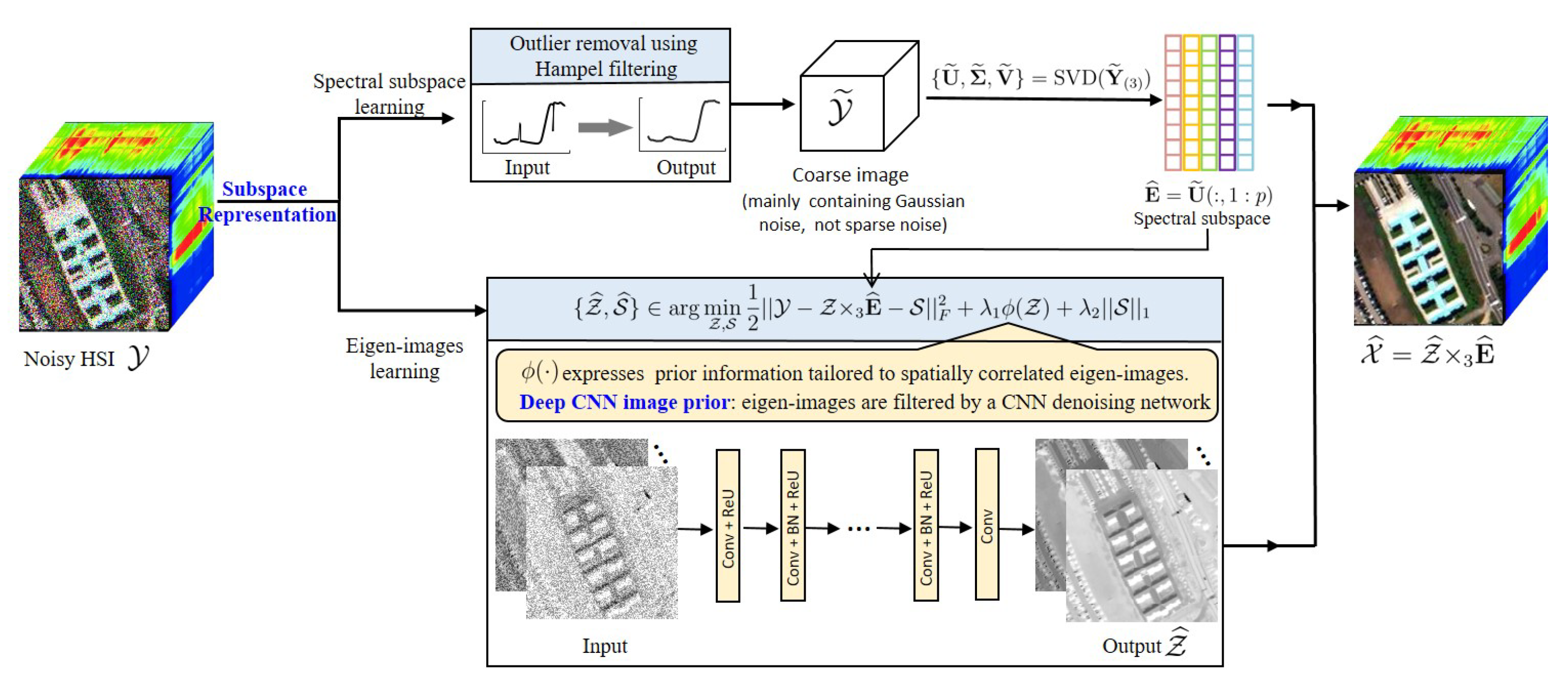
  • Instead of estimating the subspace basis and the corresponding coefficients of HSIs jointly and iteratively, we decouple the estimation of the subspace basis and the corresponding coefficients. A new subspace learning method, which works independently from coefficient estimation and is robust to mixed noise, is proposed.
  • An image prior extracted from a state-of-the-art neural denoising network, FFDNet, is seamlessly embedded within our HSI mixed noise removal framework, which is a successful combination of the traditional machine learning technique and deep learning technique.
This paper is organized as follows. Section 2 formally introduces a mixed noise removal method—HySuDeep. Section 3 extends the proposed method to address mixed noise containing non-i.i.d. Gaussian noise. Section 4 and Section 5 show and analyze the experimental results of the proposed method and the comparison methods. Finally, we present a conclusion of this paper in Section 6.

2. Problem Formulation

Some notations and tensor operations used in this paper and their definitions are provided in Table 1.

2.1. Observation Model

Let X R r × c × n b denote an underlying clean HSI with r × c pixels and n b bands. Assuming that noise is additive, we can write an observation model as
Y = X + S + G ,
where Y , S , G R r × c × n b are observed HSI data, sparse noise, and Gaussian noise, respectively. Elements in G are assumed to be i.i.d. Gaussian with zero-mean and variance σ 2 . Non-i.i.d. noise is discussed in Section 3.

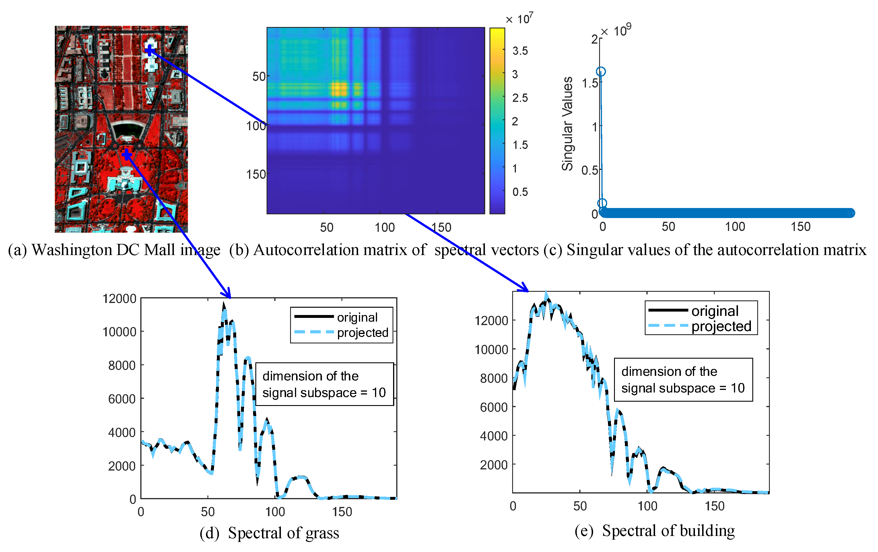
2.2. Subspace Representation of HSIs

The high correlation in the spectral domain of HSIs implies that spectral vectors (i.e., mode-3 vectors) of an HSI X can be well represented in a low-dimensional subspace [1,8,19]. We take a cropped Washington DC Mall image (shown in Figure 1a) as an example. To analyze the correlation of pixel values in the spectral domain, we obtained the autocorrelation matrix of its spectral vectors by computing E [ X ( 3 ) X ( 3 ) T ] . From Figure 1b, we can see that the first 100 bands are highly correlated. Due to the high spectral correlation, the autocorrelation matrix can be approximated by a low-rank matrix. The low-rankness may also be inferred in Figure 1c, where the first two singular values (the largest) dominate all other singular values, which decrease to near-zero rapidly. From Figure 1d,e, we can see that two spectral vectors of size 191 can be well approximated by vectors in a subspace with a dimension of 10.
Based on the subspace representation of spectral vectors, we write
X = Z × 3 E + Ξ ,
with E R n b × p ( p n b ), Z R r × c × p , and Ξ R r × c × n b . Matrix E holds an orthogonal basis for the signal subspace, and the entries of Z are representation coefficients of X with respect to E . Hereafter, mode-3 slices of Z are termed the eigenimages. Tensor Ξ represents residuals of a low-dimensional representation of X . When SVD is adopted, most of the image variation can be compactly represented in a low-dimensional subspace, and the residual tensor contains a small amount of image energy. Thus, we omit Ξ when reconstructing the image; that is, X = Z × 3 E . Figure 2 illustrates the subspace representation of a hyperspectral image. The observation model (1) can be written as
Y = Z × 3 E + S + G .
The subspace representation of spectral vectors has been demonstrated to be a powerful tool for solving some hyperspectral inverse problems, such as hyperspectral image super-resolution [33], hyperspectral image segmentation [34], hyperspectral image classification [35], and hyperspectral unmixing [36]. In this paper, we propose a hyperspectral image mixed noise removal method using subspace representation and deep CNN Image prior (HySuDeep), the flowchart of which is illustrated in Figure 3.
However, for the hyperspectral mixed noise removal problem, the challenge of exploiting subspace representation lies in the estimation of the subspace from observations corrupted not only by Gaussian noise but also by sparse noise.

2.3. Subspace Learning against Mixed Noise

When noise in an observed HSI is approximately Gaussian distributed, the subspace of the underlying clean image can be estimated easily from the noisy image by performing SVD on the noisy image matrix; that is, { U , Σ , V } = SVD ( Y ( 3 ) ) . The estimated subspace is spanned by k eigenvectors corresponding to the k largest eigenvalues; that is, E ^ = [ U ] : , 1 : k , where the subscript ( : , 1 : k ) means extracting the first k columns from a matrix.
However, when noise is a mixture of Gaussian noise and stripe noise, performing SVD on a noisy image matrix is not an optimal way to learn the spectral subspace. SVD aims to find the most important dimensions in the data by finding the directions of maximum variance, and the addition of i.i.d. Gaussian noise increases the variance of each dimension uniformly (thus, it does not change the order of singular values and consequently does not change the estimation of subspace), whereas the addition of stripes increases the variance of each dimension non-uniformly (thus, it does change the order of singular values). Experimental analysis is given in Section 4.3.
One of our contributions is to estimate the spectral subspace from observations corrupted by mixed noise and thus propose an efficient denoising method, which does not need to estimate spectral subspace iteratively.

2.3.1. Outlier Removal Using Hampel Filtering

Since the existence of sparse noise significantly disturbs the identification of signal subspace, we may estimate a coarse image by removing the sparse noise from observations. An outlier removal step applying Hampel filtering to spectral vectors of the observed image is introduced below.
Given a spectral vector of observed HSI, denoted as y = [ y 1 , y 2 , , y n b ] T R n b , and a sliding window of length q, we define the point-to-point median and median absolute deviation (MAD) estimates for the samples in the ith band using
m i = median ( y i q , y i q + 1 , y i q + 2 , , y i , , y i + q 2 , y i + q 1 , y i + q ) ,
and
MAD = median ( | y i q m i | , , | y i + q m i | ) ,
respectively. The standard deviation (denoted as σ i , M A D ) is estimated by scaling the local median absolute deviation (MAD) by a factor of κ = 1 / ( 2 erf 1 ( 1 / 2 ) ) 1.4826 :
σ i , M A D = κ MAD .
The Hampel filtering is a variation of the three-sigma rule of statistics, which is robust against outliers. If a sample y i is such that
| y i m i | > n σ σ i , M A D
for a given threshold n σ , then the Hampel filtering declares y i an outlier and replaces it with m i ; that is,
y ˜ i = m i if | y i m i | > n σ σ i , M A D . y i otherwise .
Here, we simply set n σ to 3.
The coarse image Y ˜ is obtained by applying the Hampel filtering (8) to each spectral vector of the observed image. We remark that although the Hampel filtering can detect the positions of impulse noise and stripes well, it may not produce exact spectral estimates for the polluted pixels. Thus, the goal of performing the Hampel filtering on the observed image is to obtain a coarse image for subspace learning.

2.3.2. Subspace Identification

Given the coarse image Y ˜ (mainly containing Gaussian noise, not sparse noise), the subspace basis can be directly obtained by performing SVD on Y ˜ , as Y ˜ mainly contains Gaussian noise which is independent and identically distributed (i.i.d.). That is, the signal subspace is approximately spanned by the first p left-singular vectors of Y ˜ :
E ^ = U ˜ ( : , 1 : p ) ,
where U ˜ R n b × n b is an orthogonal matrix and { U ˜ , Σ ˜ , V ˜ } = SVD ( Y ˜ ( 3 ) ) with singular values in Σ ˜ ordered by non-increasing magnitude. The dimension of subspace, p, can be automatically estimated by the HySime method [37].

2.4. Fast Eigenimage Learning

2.4.1. Objective Function

Given the estimate of spectral subspace and the noise assumption (i.e., a mixture of i.i.d. Gaussian noise and sparse noise), we estimate the unknown variables, Z and S , in (3) by solving
{ Z ^ , S ^ } arg min Z , S 1 2 | | Y Z × 3 E ^ S | | F 2 + λ 1 ϕ ( Z ) + λ 2 | | S | | 1 .
The first term on the above optimization problem is derived from the observation model (3). The third term is a regularizer with respect to matrix S . The 1 norm of S , given by S 1 = i = 1 r j = 1 c k = 1 n b | S ( i , j , k ) | , promotes the sparsity of S . Finally, λ 1 , λ 2 0 are regularization parameters that trade off the importance of the respective regularizers. If the ϕ is a convex function, then the optimization (10) is a convex problem.
The second term in the optimization problem (10) is a regularization expressing prior information tailored to spatially correlated eigenimages [8,17]. We use the plug-and-play technique [29,30] to assign a prior for eigenimages; rather than investing efforts in designing new regularization for eigenimages, we can plug an image prior extracted from an off-the-shelf denoiser conceived for natural images. A deep image prior extracted from a CNN-based denoising network, FFDnet, is employed, and thus an explicit definition of the function ϕ ( · ) is not given in optimization (10). More detailed analysis with regard to the deep prior ϕ ( · ) can be found in Section 2.4.3.
Let A = concat ( [ Z , S ] , 3 ) be a r × c × ( p + n b ) tensor that concatenates the eigenimages Z and the sparse noise S along the third dimension. The optimization problem (10) can be rewritten as
A ^ arg min A 1 2 Y A × 3 [ E ^ , I n b ] F 2 + λ 1 ϕ ( A × 3 [ I p , 0 ( p × n b ) ] ) + λ 2 A × 3 [ 0 ( n b × p ) , I n b ] 1 ,
where I a denotes an identity matrix of size a and 0 ( a × b ) is a zero matrix of size a × b .

2.4.2. Solver

The optimization problem (11) can be solved by the constrained-split augmented Lagrangian shrinkage algorithm (C-SALSA) [38,39]. C-SALSA is an instance of an alternating direction method of multipliers (ADMM) [40] that was developed to solve the constrained optimization formulation of regularized image restoration. By using variable splitting, we can convert the original optimization into a constrained one:
min A , V 1 , V 2 , V 3 1 2 Y V 1 F 2 + λ 1 ϕ ( V 2 ) + λ 2 V 3 1 s . t . V 1 = A × 3 [ E ^ , I n b ] V 2 = A × 3 [ I p , 0 ( p × n b ) ] V 3 = A × 3 [ 0 ( n b × p ) , I n b ] .
The augmented Lagrangian function of the above optimization is
L ( A , V 1 , V 2 , V 3 , D 1 , D 2 , D 3 ) = 1 2 Y V 1 F 2 + λ 1 ϕ ( V 2 ) + λ 2 V 3 1 + μ 1 2 V 1 A × 3 [ E ^ , I n b ] D 1 F 2 + μ 2 2 V 2 A × 3 [ I p , 0 ( p × n b ) ] D 2 F 2 + μ 3 2 V 3 A × 3 [ 0 ( n b × p ) , I n b ] D 3 F 2 , + constant
where μ 1 , μ 2 , μ 3 > 0 are C-SALSA penalty parameters.
The application of C-SALSA to (13) leads to Algorithm 1.  A MATLAB demo of the proposed HySuDeep method will available at https://github.com/LinaZhuang (accessed on 8 October 2021).
Algorithm 1HySuDeep for mixed noise containing i.i.d. Gaussian noise
1:
Set k = 0 , choose μ 1 , μ 2 , μ 3 > 0 , V 1 , 0 , V 2 , 0 , D 1 , 0 , D 2 , 0 .
2:
repeat
3:
A k + 1 = arg min A μ 1 2 V 1 , k A × 3 [ E ^ , I n b ] D 1 , k F 2 + μ 2 2 V 2 , k A × 3 [ I p , 0 ( p × n b ) ] D 2 , k F 2 + μ 3 2 V 3 , k A × 3 [ 0 ( n b × p ) , I n b ] D 3 , k F 2  
4:
V 1 , k + 1 = arg min V 1 1 2 Y V 1 F 2 + μ 1 2 V 1 A k + 1 × 3 [ E ^ , I n b ] D 1 , k F 2  
5:
V 2 , k + 1 = arg min V 2 λ 1 ϕ ( V 2 ) + μ 2 2 V 2 A k + 1 × 3 [ I p , 0 ( p × n b ) ] D 2 , k F 2  
6:
V 3 , k + 1 = arg min V 3 λ 2 V 3 T 1 + μ 3 2 V 3 A k + 1 × 3 [ 0 ( n b × p ) , I n b ] D 3 , k F 2  
7:
D 1 , k + 1 = D 1 , k ( V 1 , k + 1 A k + 1 × 3 [ E ^ , I n b ] )  
8:
D 2 , k + 1 = D 2 , k ( V 2 , k + 1 A k + 1 × 3 [ I p , 0 ( p × n b ) ] )  
9:
D 3 , k + 1 = D 3 , k ( V 3 , k + 1 A k + 1 × 3 [ 0 ( n b × p ) , I n b ] )  
10:
k k + 1
11:
until stopping criterion is satisfied.
The optimizations with regard to A and V 1 (on lines 3 and 4 of Algorithm 1) are quadratic problems, whose solutions are given by
A k + 1 =   ( μ 1 ( V 1 D 1 ) × 3 [ E ^ , I n b ] T + μ 2 ( V 2 D 2 ) × 3       [ I p , 0 ( p × n b ) ] T + μ 3 ( V 3 D 3 ) × 3 [ 0 ( n b × p ) , I n b ] T ) × 3       ( μ 1 [ E ^ , I n b ] T [ E ^ , I n b ] + μ 2 [ I p , 0 ( p × n b ) ] T       [ I p , 0 ( p × n b ) ] + μ 3 [ 0 ( n b × p ) , I n b ] T [ 0 ( n b × p ) , I n b ] ) 1
(for line 3) and
V 1 , k + 1 = ( 1 + μ 1 ) 1 Y + μ 1 ( A k + 1 × 3 [ E ^ , I n b ] + D 1 , k ) .
(for line 4).
Line 6 of Algorithm 1 is a proximity operator of the 1 norm applied to V 3 , k = A k + 1 × 3 [ 0 ( n b × p ) , I n b ] + D 3 , k . It can be solved by an element-wise soft-threshold function; that is,
V 3 , k + 1 = arg min V 3 λ 2 V 3 1 + μ 3 2 V 3 V 3 , k F 2 = [ thresh ( V 3 , k ( i , j , k ) , λ / μ 3 ) , i = 1 , , r , j = 1 , , c , k = 1 , , n b ] ,
and threshold ( x , τ ) returns the soft thresholding of x (where τ is the threshold value) [41]:
x max ( | x | τ , 0 ) max ( | x | τ , 0 ) + τ x .
Line 5 of Algorithm 1 is a proximity operator of ϕ applied to V 2 , k = A k + 1 × 3 [ I p , 0 ( p × n b ) ] + D 2 , k . As the scaled Lagrange multiplier D 2 , k tends to 0 as the C-SALSA iteration goes on, V 2 , k tends to be close to Z k + 1 . Considering that orthogonal projection is a decorrelation transformation and mode-3 slices of Z tend to be decorrelated, it is reasonable to decouple ϕ ( · ) with respect to the mode-3 slices; that is,
ϕ ( V 2 , k ) = i = 1 p ϕ i V 2 , k ( : , : , i ) ,
where V 2 , k ( : , : , i ) denotes the ith mode-3 slice. The solution of the subproblem on line 5 can be decoupled with regard to mode-3 slices of V 2 , k and can be written as
V 2 , k + 1 = Ψ λ 1 ϕ / μ 2 ( V 2 , k ) = Ψ λ 1 ϕ 1 / μ 2 V 2 , k ( : , : , 1 ) Ψ λ 1 ϕ p / μ 2 V 2 , k ( : , : , p )
where
Ψ λ ϕ i ( U ) = arg min X 1 2 X U F 2 + λ ϕ i ( X )
is the so-called Moreau proximity operator (MPO) [42] of ϕ or the denoising operator.

2.4.3. Plug-and-Play Prior, ϕ ( · )

Instead of investing great effort in conceiving a new eigenimage regularization ϕ i ( X ) , we make use of the plug-and-play (PnP) prior [8,29,30]. The PnP tool is a powerful framework that solves an inverse image problem by directly using an existing regularizer from a state-of-the-art image denoiser. The PnP framework has been applied to hyperspectral image fusion, spectral unmixing, hyperspectral image inpainting, and anomaly detection, and produces surprisingly good image recovery results. Inspired by these successful applications of PnP, we plug the prior of a deep denoising network, FFDnet [24], into (18), leading to
V ^ 2 , k ( : , : , i ) FFDNet ( V 2 , k ( : , : , i ) ) ,
where FFDNet ( · ) represents the network and outputs a denoised image. It is worth noting that other state-of-the-art image denoisers can also be plugged in (18). We choose FFDNet in this work based on the following considerations: (a) deep-learning-based FFDNet is much faster than other machine learning-based denoisers as long as it has been well trained and (b) FFDNet is flexible and able to address images with various noise levels without retraining the network.
Since the denoiser FFDNet, plugged into the subproblem with regard to V 2 , is not a proximity operator, we do not have a theoretical convergence guaranteed for the implemented variant of C-SALSA. However, impressive performances using plugged non-convex regularizations have been observed in a number of inverse problems [19,43,44]. The numerical convergence of the proposed HySuDeep is analyzed in Section 4.5.

2.5. HSI Recovery

After estimating Z ^ , the denoised image is obtained as follows:
X ^ = Z ^ × 3 E ^ .

3. Model Extension to Non-i.i.d. Gaussian Noise

Gaussian noise in the observation model (1) is assumed to be i.i.d., meaning that the model is simplified and we can focus on the discussion of the image structure. Let C λ = E [ n i n i T ] (where n i is a generic column of unfolded mode-3 matrix N ( 3 ) ) define the covariance matrix of the spectral noise. We have C λ = σ 2 I n b when the noise is i.i.d.
However, we remark that Gaussian noise in real HSIs tends to be non-i.i.d.; that is, it is pixel-wise independent but band-wise dependent. Before implementing denoising according to model (1), we need to convert the non-i.i.d. scenario into an i.i.d. scenario by implementing data whitening:
Y ¯ = Y × 3 C λ 1 ,
where C λ and C λ 1 denote the square root of C λ and the inverse of C λ , respectively.
The estimate of the covariance matrix, C λ , is challenging when noise in observations is a mixture of Gaussian and sparse noise. If the HSI is only corrupted by Gaussian noise, then the noise covariance matrix can be estimated by exploiting the spectral correlation of HSI. The spectrally uncorrelated components extracted from the HSI are considered as Gaussian noise, whose covariance matrix can be computed easily. This problem has been studied deeply, and we refer readers to representative works [37,45]. However, when the noise in the image is a mixture of Gaussian noise and sparse noise, the spectrally uncorrelated components extracted from the HSI are mixed noise, instead of single Gaussian noise. To solve this problem, we propose a method to split two kinds of noise and estimate C λ in two steps, as listed below:
  • Estimate a coarse image, Y ˜ , by removing the sparse noise from observation. A outlier removal step applying Hampel filtering to spectral vectors of the observed image is given in ( 8 ) .
  • We apply linear regression to each band of the image Y ˜ ; i.e., each band is represented as a linear combination of the remaining bands [37]. That is,
    [ Y ˜ ( 3 ) T ] : , i = [ Y ˜ ( 3 ) T ] α i β i + ξ i ,
    where Y ˜ ( 3 ) T denotes the transpose of the mode-3 unfolding matrix Y ˜ ( 3 ) , the subscript [ · ] : , i means extracting the ith column from a matrix, a matrix with the subscript [ · ] α i means the matrix including all columns except ith column, β i R n b 1 denotes regression coefficients, and ξ ^ i R n denotes regression error.
    The regression coefficients β i can be estimated by the least squares method; i.e.,
    β ^ = arg min β [ Y ˜ ( 3 ) T ] : , i [ Y ˜ ( 3 ) T ] α i β i F 2 .
    Given β ^ , the regression error, ξ ^ i , is computed by
    ξ ^ i = [ Y ˜ ( 3 ) T ] : , i [ Y ˜ ( 3 ) T ] α i β ^ i .
    The regression errors are taken as a coarse estimate of the Gaussian noise; thus, its covariance matrix, C λ = diag ( [ σ 1 2 , σ 2 2 , , σ n b 2 ] ) , can be estimated by
    σ i 2 = var ( ξ ^ i ) ,
    where var ( · ) is a function computing the variance of the elements of the input vector.
Given the estimate of C λ , we can convert band-dependent Gaussian noise to i.i.d. Gaussian noise via (21). Here, we analyze the impact of image conversion on Gaussian noise. Given the image conversion,
Y ¯ = X × 3 C λ 1 + S × 3 C λ 1 + G × 3 C λ 1 ,
we can compute the spectral covariance of the Gaussian noise in the converted image as follows:
C ¯ λ = E [ C λ 1 n i ( C λ 1 n i ) T ] = C λ 1 E [ n i n i T ] C λ 1 T = C λ 1 C λ C λ 1 T = I .
From (27), we can see that after image conversion, the Gaussian noise is i.i.d. and standard distributed, which meets the noise assumption in model (1); thus, the converted image, Y ¯ , can be denoised as discussed in Section 2. Finally, we reconstruct the clean image as follows:
X ^ = X ¯ ^ × 3 C λ ,
where X ¯ ^ is the estimated clean version of image Y ¯ .
The pseudocode in Algorithm 2 shows how HySuDeep is implemented to reduce mixed noise for an HSI. Given an HIS of size r (rows) × c (columns) × n b (bands) with subspace dimension p ( p n b ), the computational complexity of obtaining a coarse image Y ˜ in line 2 and C λ in line 3 is O ( r * c * n b * q * log q ) and O ( r * c * n b 3 ) , respectively. The Gaussian noise-whitening in line 4, its inverse transformation in line 8, and the image reconstruction step in line 7 have the same computational complexity; that is, O ( r × c × n b 2 ) . The estimation of the spectral subspace in line 5 and eigenimages in line 6, respectively, cost O ( r 2 * c 2 * n b ) and O ( r * c * ( p + n b ) 2 + ( p + n b ) 3 + p * d ) . Here, d represents the computational complexity of denoising an eigenimage using FFDNet. Consequently, the overall computational complexity of HySuDeep is O ( r * c * n b 3 + r 2 * c 2 * n b + p * d ) .
Algorithm 2HySuDeep for mixed noise containing non-i.i.d. Gaussian noise
1:
Input a noisy HSI, Y , and parameter λ 2 .
2:
Estimate a coarse image Y ˜ via (8).
3:
Estimate C λ from Y ˜ via (25).
4:
Obtain an whitened image Y ¯ using (21).
5:
Denoise the whitened image Y ¯ using Algorithm 1, and obtain X ¯ ^ .
6:
Compute X ^ = X ¯ ^ × 3 C λ , an estimate of the clean HSI.

4. Experiments with Simulated Images

Experiments were carried out on three simulated datasets to evaluate the performance of the proposed HySuDeep method compared with six state-of-the-art denoising methods for HSI mixed noise removal.

4.1. Simulation of Noisy Images and Comparisons

4.1.1. Simulation of Noisy Images
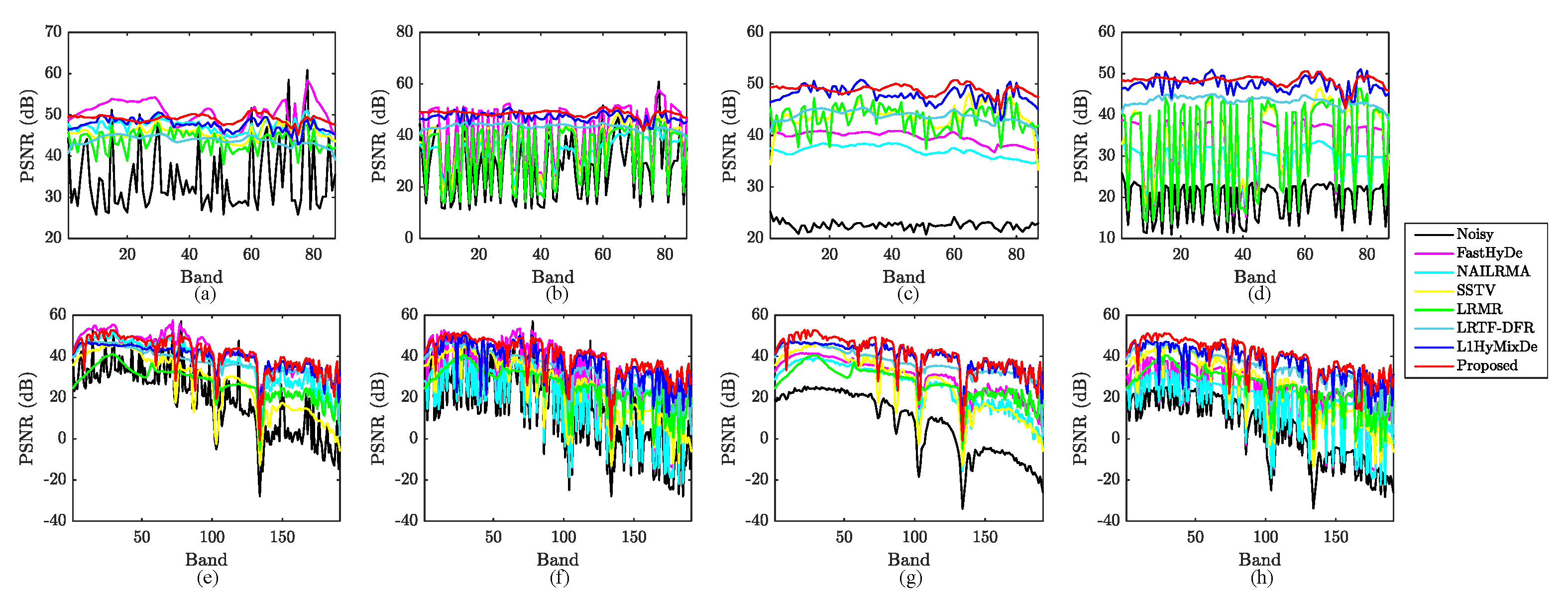
Three public hyperspectral datasets (shown in Figure 4a–c) were employed to simulate the noisy images. Following the same procedure in [32], we generated noisy HSIs of Pavia University data (of size 310 (rows) × 250 (columns) × 87 (bands)), a subregion of Washington DC Mall data (of size 150 (rows) × 200 (columns) × 191 (bands)), and Terrain data (of size 500 (rows) × 307 (columns) × 166 (bands)).
For the first two datasets, we removed bands that were severely corrupted by water vapor in the atmosphere. To obtain relatively clean images, we projected spectral vectors of each image onto a subspace spanned by eight principal eigenvectors of each image. The projection of each image was considered to be a clean image. To simulate noisy HSIs, we added four kinds of additive noise into images as follows:
Case 1 (Gaussian non-i.i.d. noise): Synthetic data with Gaussian noise. The noise in ith pixel vector g i N ( 0 , D 2 ) , where D is a diagonal matrix with diagonal elements sampled from a uniform distribution U ( 0 , 0.01 ) .
Case 2 (Gaussian noise + stripes): Synthetic data with Gaussian noise (described in case 1) and oblique stripe noise randomly affecting 30% of the bands and, for each band, about 10% of the pixels, at random.
Case 3 (Gaussian noise + “Salt and Pepper” noise): Synthetic data with Gaussian noise (described in case 1) and “Salt and Pepper” noise with a noise density of 0.5%, meaning approximately 0.5% of elements in X are affected.
Case 4 (Gaussian noise + stripes + “Salt and Pepper” noise): Synthetic data with Gaussian noise (described in case 1), random oblique stripes (described in case 2) and “Salt and Pepper” noise (described in case 3).
To evaluate the impact of denoising methods on the hyperspectral unmixing task, we simulated a clean semi-real HSI based on the publically available Terrain image (Figure 4c) following generation steps in [36]. A MATLAB demo used to generate a semi-real HSI is available at https://github.com/LinaZhuang/NMF-QMV_demo, accessed on 8 October 2021. The original Terrain image has a size of 500 (rows) × 307 (columns) × 166 (bands) and is mainly composed of soil, tree, grass, and shadow. The number of endmembers is empirically set to 5, as performed in [36,46,47]. Briefly, a clean Terrain image was synthesized based on a linear mixing model [1]; i.e., X = A × 3 M , where M and A are endmembers and abundances, respectively, estimated from the original Terrain image. Next, we generated a noisy Terrain HSI by adding the Gaussian noise and oblique stripe noise (as described in case 2)—i.e., Y = A × 3 M + S + G —yielding an MPSNR of 28.90 dB.

4.1.2. Comparisons

To thoroughly evaluate the performance of the proposed method, six state-of-the-art HSI denoising methods were selected for comparison: the fast hyperspectral denoising method (FastHyDe) [8], the noise-adjusted iterative low-rank matrix approximation method (NAIRLMA) [48], the spatio-spectral total variation based method (SSTV) [49], the low-rank matrix recovery method (LRMR) [15], double-factor-regularized low-rank tensor factorization (LRTF-DFR) [21], and the 1 -norm based hyperspectral mixed noise denoising method (L1HyMixDe) [32]. These compared methods were carefully selected. The FastHyDe served as a benchmark to see whether mixed noise could be simply addressed by Gaussian denoisers. The NAIRLMA, SSTV, and LRMR are from highly cited papers working on hyperspectral mixed noise based on low-rank and sparse representations. The LRTF-DFR and L1HyMixDe methods are subspace representation methods and remove noise by filtering the subspace coefficients of HSIs. All experiments were implemented in MATLAB (R2016a) on Windows 10 with an Intel Core i7-7700HQ 2.8-GHz processor and 24 GB RAM. A MATLAB demo of this work will be available at https://github.com/LinaZhuang, (accessed on 8 October 2021) for the sake of reproducibility.
The size of the sliding window in the Hampel filter, q, was fixed to 7. The dimension of the subspace, p, for FastHyDe, LRTF-DFR, L1HyMixDe, and HySuDeep methods was estimated by HySime [37] automatically. The other parameters of FastHyDe, NAILRMA, LRTF-DFR, and L1HyMixDe were set as suggested in their original references. We fine-tuned the parameters λ and μ in SSTV and parameters r and s in LRMR to obtain the optimal results.
For quantitative assessment, the peak signal-to-noise ratio (PSNR) index, the structural similarity (SSIM) index, and the feature similarity (FSIM) index of each band were calculated. The mean PSNR (MPSNR), mean SSIM (MSSIM), and mean FSIM (MFSIM) of the proposed and compared methods on Pavia University Data and Washington DC Mall Data are presented in Table 2, where we have highlighted the best results in bold.

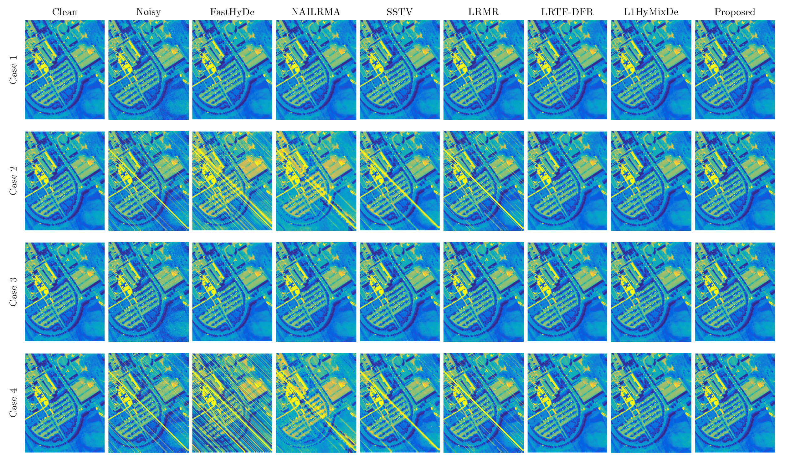
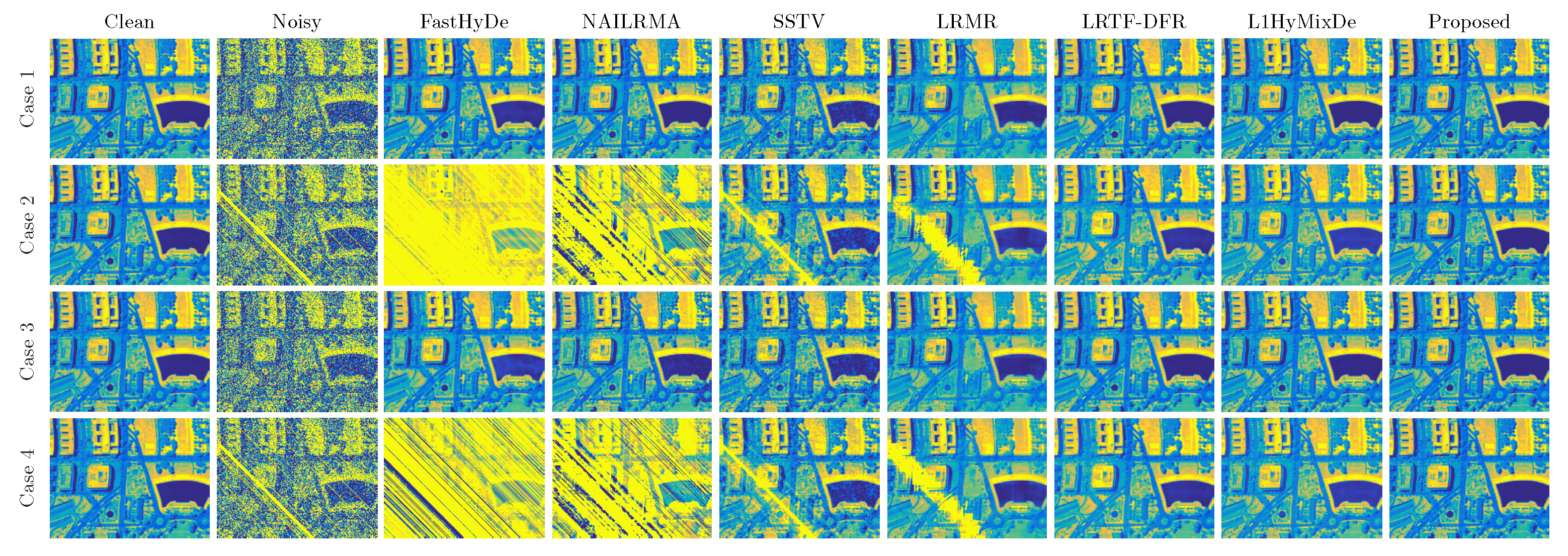
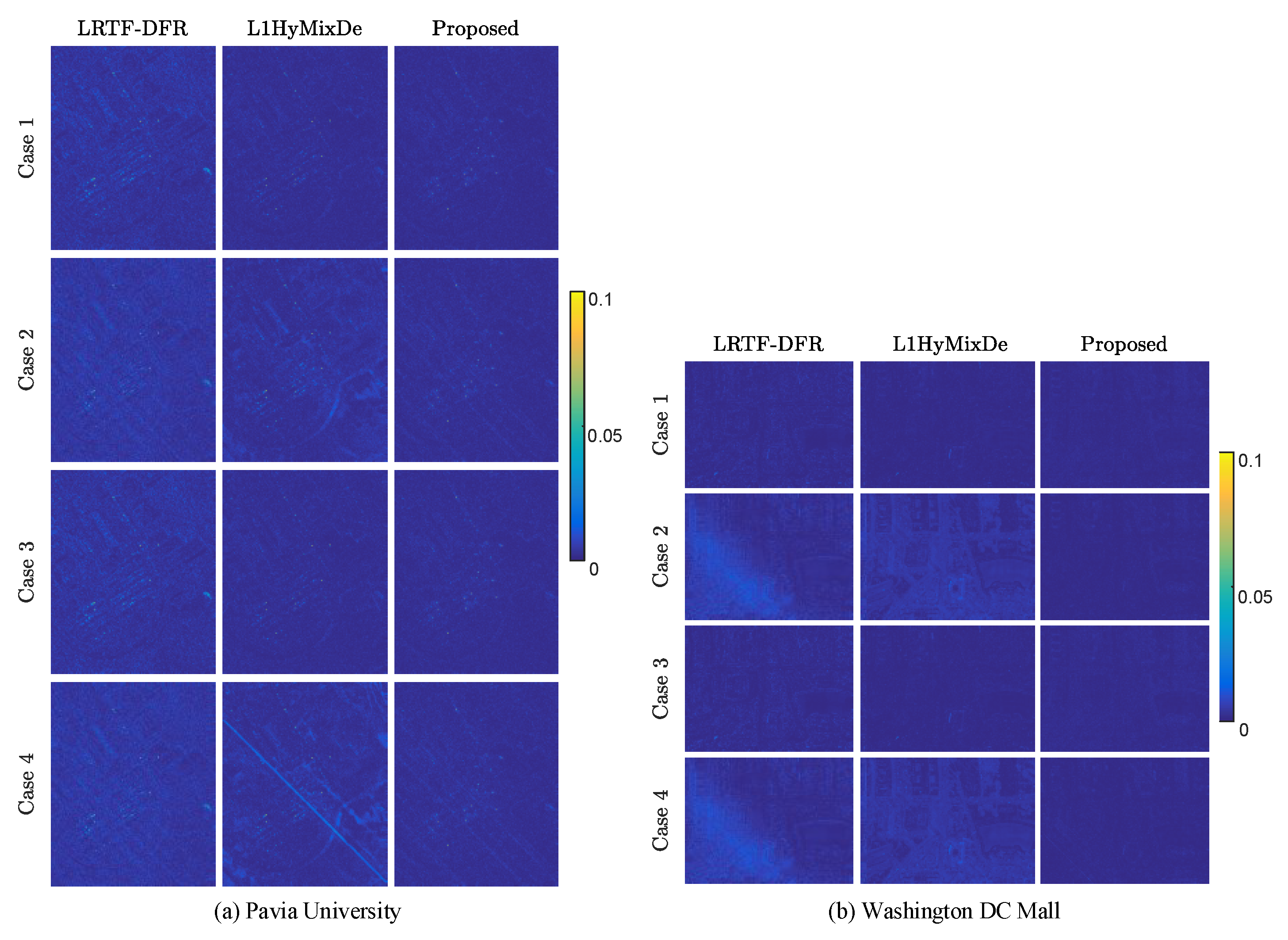
4.2. Mixed Noise Removal

We compare the proposed method HySuDeep with FastHyDe [8], NAILRMA [48], SSTV [49], LRMR [15], LRTF-DFR [21], and L1HyMixDe [32] methods in terms of MPSNR, MSSIM, and MFSIM (provided in Table 2 and Table 3). The band-wise PSNR is depicted in Figure 5 for quantitative assessment.
Among the compared methods, only FastHyDe is shown to address pure Gaussian noise, not mixed noise. We include FastHyDe to evaluate whether mixed noise can be reduced by a simple Gaussian denoiser. As shown in Table 2, FastHyDe outperformed other methods in case 1 (where HSIs are corrupted by only Gaussian noise). However, when the images were contaminated by mixed noise in Cases 2–4, the results of FastHyDe show that heavy mixed noise cannot be reduced well by a Gaussian denoiser. The existence of mixed noise in HSIs calls for effective denoising techniques.
To address mixed noise, an additive term is usually introduced to model sparse noise so that the entries in the data fidelity term, ( Y X S ) , follow Gaussian distributions. The proposed HySuDeep, NAIRLMA, SSTV, LRMR, and LRTF-DFR methods fall in this line of research. The critical differences among these methods are the regularizations imposed on the HSI, X . SSTV minimizes the total variation of the HSI in the spectral–spatial domain. NAILRMR and LRMR impose spectral low-rankness in spatial patches of the image. LRTF-DFR and the proposed HySuDeep both enforce the low-rankness of spectral vectors by subspace representation. To exploit the spatial correlation of eigenimages, LRTF-DFR minimizes the spatial difference (i.e., total variation) of eigenimages, while HySuDeep uses a CNN-regularization (i.e., a deep image prior extracted from a CNN network).
The proposed method uniformly yields the best results in Cases 2–4, as shown in Table 2 and Table 3. The main reason is that, compared with SSTV, NAILRMR, LRMR, LRTF-DFR, and L1HyMixDe methods, our method uses a more efficient spatial regularization term. Although the CNN regularization works like a black box, we can see its superiority over TV regularization (used in SSTV and LRTF-DFR) and patch-based regularization (used in NAILRMA, LRMR, and L1HyMixDe) from Table 2 and Table 3. Furthermore, HySuDeep is similar to the L1HyMixDe method in terms of using subspace representations of spectral vectors and imposing a regularization on representation coefficients. Table 2 and Table 3 show that HySuDeep achieves better results than L1HyMixDe. The difference is caused by the accuracy of spectral subspace learning. Compared with L1HyMixDe, HySuDeep elaborates an outlier removal operator, which improves the estimates of subspace E ^ (see discussion in Section 4.3).
For visual comparison, we display the 37th band of Pavia University data and the 126th band of Washington DC Mall data in Figure 6 and Figure 7, respectively. For case 1 (Gaussian noise), all methods can reduce noise significantly. As shown in Figure 6 and Figure 7, SSTV and LRMR are able to remove light stripes, but still leave some wide stripes. Heavy noise still remains in the results of NAILRMA and FastHyDe. LRTF-DFR, L1HyMixDe, and HySuDeep methods visually yield comparable results in Figure 6 and Figure 7. To show their differences, we generated and presented the residual images in Figure 8a,b, where we can see the results of proposed HySuDeep contain less residual compared with LRTF-DFR and L1HyMixDe.

4.3. Subspace Learning against Mixed Noise

One of the contributions of this paper is the introduction of an orthogonal subspace identification method that is robust to mixed noise. We conducted experiments using simulated images to compare the proposed subspace learning method with representative subspace learning methods: namely, SVD, RPCA, L1HyMixDe [32], and HySime [37]. Results are reported in Table 4, where we show two metrics, namely γ 1 = X × 3 E ^ T × 3 E ^ F 2 / X F 2 and γ 2 = N × 3 E ^ T × 3 E ^ F 2 / N F 2 , measuring the relative power of the clean spectral vectors and noise lying in the estimated subspace, respectively.
In Case 1, two images were corrupted only by Gaussian noise, and values of γ 1 for all methods are higher than 0.9993, implying that all the methods can estimate a subspace representing image signal very well. Case 3 shows results similar to Case 1; that is, all the methods achieve relatively high γ 1 . We conclude that when noise is Gaussian distributed or a mixture of Gaussian and “Salt and Pepper” noise, signal subspace learning is not a challenging task and we can simply use SVD. The reason is that Gaussian noise and “Salt and Pepper” noise are randomly and uniformly distributed in each channel; thus, the noise increases singular values in the direction of each eigenvector almost uniformly and does not change the order of the singular values of clean images. The signal subspace is approximately spanned by p singular vectors of the noisy image corresponding to the largest p singular values.
However, subspace learning from noisy images in Case 2 and Case 4 is challenging and we cannot simply use SVD because the stripe noise usually exist in specific channels, instead of being uniformly distributed in all channels. The stripe noise will significantly increase the variances of those channels affected by stripe noise. Due to the fact that SVD tends to learn a subspace representing information in channels with high variances, SVD is not suitable for Case 2 and Case 4. This inference is consistent with the results in Table 4, where SVD obtains the worst results in terms of γ 1 and γ 2 in case 2 and case 4. If we only focus on the table rows highlighted with gray color, the proposed learning method performs better than others. Among the compared methods, RPCA learns a subspace representing low-rank signal and excluding sparse noise. However, stripe noise is also low-rank [50], and RPCA cannot separate an image signal and stripes using only a low-rank regularization. HySime is conceived based on an assumption of Gaussian noise and is clearly not suitable for mixed noise. L1HyMixDe performs median filtering band by band, exploiting spatial correlation, whereas HySuDeep estimates a coarse image using Hampel filtering pixel by pixel, exploiting spectral correlation. As shown in gray rows of Table 4, HySuDeep uniformly provides the best performances.

4.4. Analysis of Regularization Parameters

There are two regularization parameters—namely, λ 1 and λ 2 —in the objective function of the proposed HySuDeep method. Controlling the trade-off between Gaussian noise reduction and detail preservation, the parameter λ 1 is related to the standard deviation of Gaussian noise, which can be estimated via (25).
The second parameter λ 2 controls the sparsity of estimation of sparse noise S . The setting of λ 2 should depend on the intensity of sparse noise. Figure 9 depicts the denoising performance of HySuDeep in the Pavia University image and in the Washington DC Mall image as a function of the value of parameter λ 2 . When the value of λ 2 is set to {1, 3, 5, 7, 9}, denoising results are acceptable in both images. Therefore, we simply set λ 2 to 3 in all experiments in this paper.

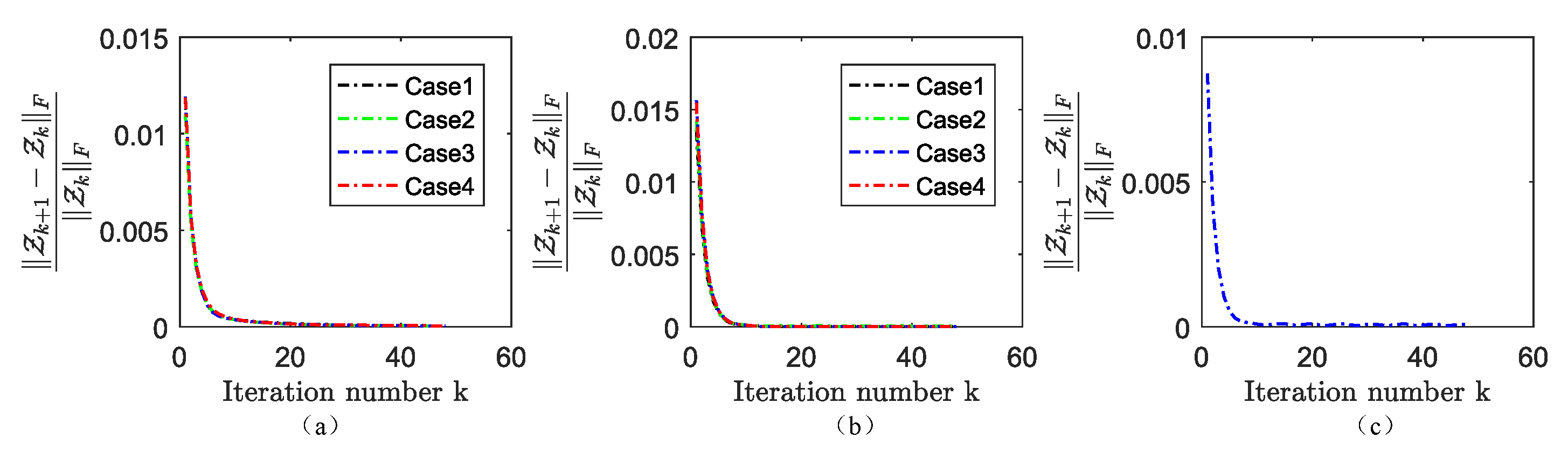
4.5. Numerical Convergence of the HySuDeep

Since CNN-regularization is incorporated into (10), the proposed HySuDeep cannot be considered as a convex optimization problem; thus, its theoretical convergence is not guaranteed. However, its numerical convergence is systematically observed when the augmented Lagrangian parameters are set to μ i = 1 ( i = 1 , 2 , 3 ) . As shown in Figure 10, the relative change converges to near zero after 15 iterations, implying the convergence of the proposed method can be numerically guaranteed.

4.6. Application in Hyperspectral Unmixing

Hyperspectral denoising is usually implemented as a preprocessing step for subsequent applications. This subsection takes hyperspectral unmixing as an example to evaluate whether the image denoising step has a positive impact on the performance of subsequent applications. Spectral unmixing mainly involves two stages: (i) identifying materials present in the scene (termed endmembers) and (ii) estimating the fraction (or abundance) of each material in each pixel. The hyperspectral unmixing task was chosen considering that the endmember extraction step can be very sensitive to sparse noise.
We first performed denoising on the Terrain image using FastHyDe, NAILRMA, SSTV, LRMR, LRTF-DFR, L1HyMixDe, and HySuDeep. The mean PSNR (MPSNR), mean SSIM (MSSIM), and mean FSIM (MFSIM) of the proposed and compared methods on Terrain image are presented in Table 3, where we have highlighted the best results in bold. Then, we unmixed the spectra of the denoised images by using vertex component analysis (VCA) [53] to estimate the endmembers and used fully constrained least squares (FCLS) [54] to estimate the abundances. Two metrics were computed: the normalized mean square error (NMSE) of endmembers A and abundances S , denoted as NMSE A and NMSE S , respectively. As reported in Table 3, LRMR, LRTF-DFR, L1HyMixDe, and HySuDeep obtain a lower NMSE of endmembers than the counterpart image without denoising processing. For images denoised by FastHyDe, NAILRMA, and SSTV, the errors in the estimates of endmembers directly result in high errors in the estimates of abundances. Among LRMR, LRTF-DFR, L1HyMixDe, and HySuDeep, the proposed HySuDeep leads to the lowest NMSE of abundances.

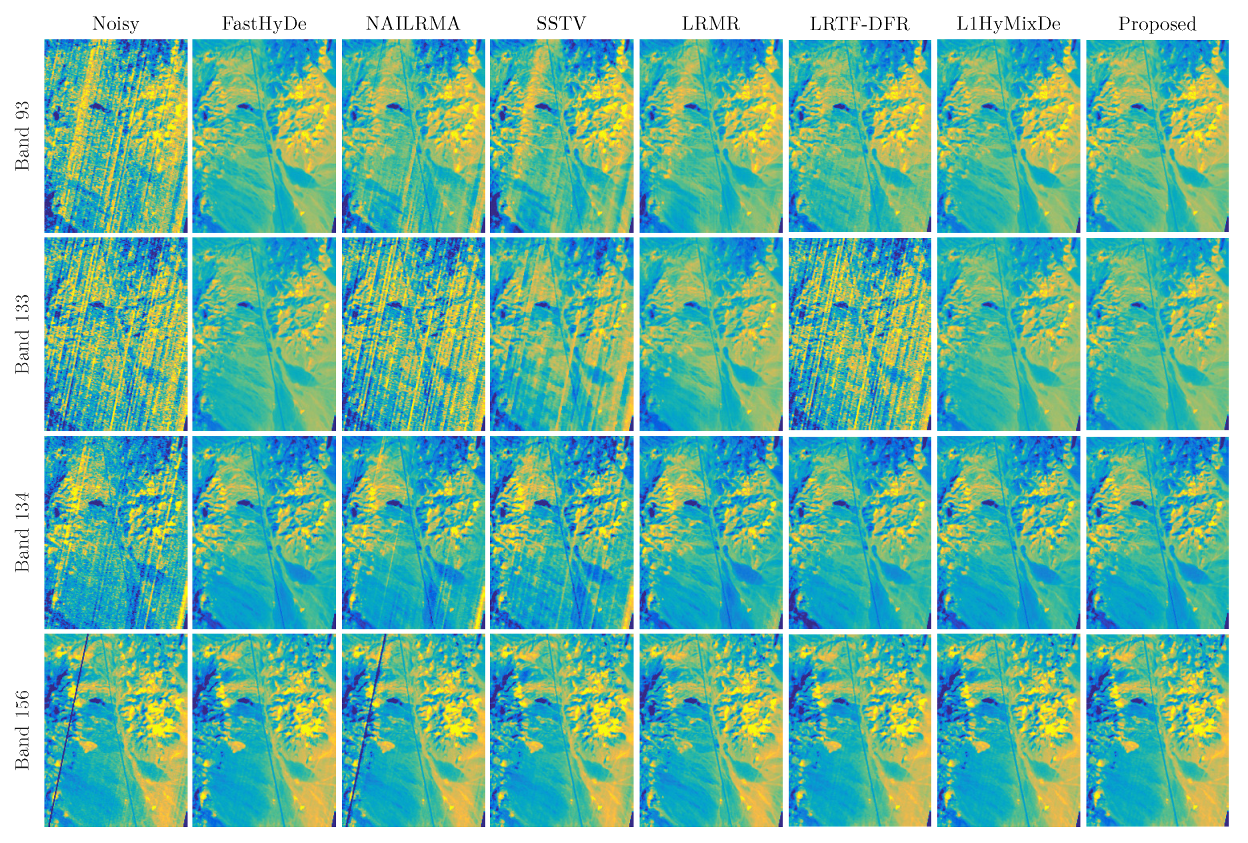
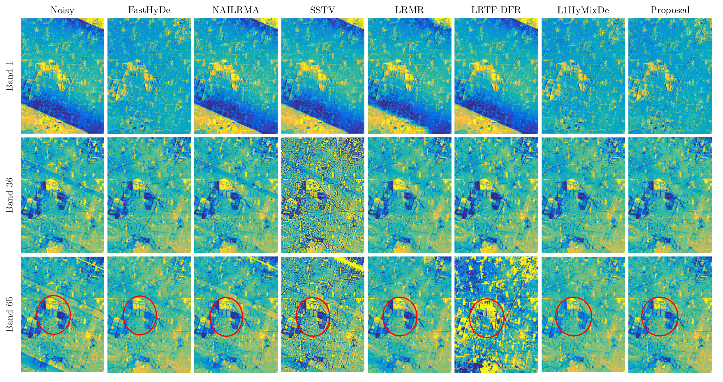
5. Experimental Results for Real Images

We evaluate the performance of the proposed method on two real HSI datasets, as shown in Figure 4d,e.

5.1. Hyperion Cuprite Dataset

The Cuprite HSI was captured at Cuprite, NV, USA, by the Hyperion sensor, which divides the spectrum from 355 nm to 2577 nm into 242 channels with a spectral resolution of 10 nm. The spatial resolution of the image is 30 m. A subregion of size 240 × 178 pixels with 177 spectral channels (after removing very low SNR channels) was cropped for the test. Four bands are shown in Figure 11, where bands 93, 133, and 134 were corrupted by severe stripes, and band 156 was affected by a dead-line. The full-resolution images of Figure 11 will be available at https://github.com/LinaZhuang, (accessed on 8 October 2021). All methods (except NAILRMA) are able to remove the dead-line in band 156. For severe stripes in the other three bands, we can see that FastHyDe, LRMR, L1HyMixDe, and HySuDeep achieved good restoration results while obvious stripes remained within the results of other methods.

5.2. Tiangong-1 Dataset

The Tiangong-1 dataset was acquired over an area of Qinghai Province, China in May 2013, by a sensor placed in the Tiangong-1 imager, which has a 75-band push broom scanner with nominal bandwidths of 23 nm short wave infrared (SWIR), covering from 800 nm to 2500 nm. A subregion image of size 351 × 253 pixels was tested. Three bands displaying strong noise are shown in Figure 12, where band 1 has severe cross-track illumination error, and bands 36 and 65 contain obvious stripes. The full-resolution images of Figure 12 will be available at https://github.com/LinaZhuang (accessed on 8 October 2021). Comparing the images before denoising and after denoising, we can see that FastHyDe, L1HyMixDe, and HySuDeep can correct the illumination error in band 1. In bands 36 and 65, FastHyDe, LRMR, L1HyMixDe, and HySuDeep can alleviate stripe noise. If we focus on band 65, our HySuDeep method obtains the visually best result considering the restoration of the areas in the red circles.

6. Conclusions

This paper introduces a hyperspectral mixed noise removal method, HySuDeep, by exploiting two important characteristics of HSIs. HySuDeep takes advantage of the spectral low-rankness of HSIs by representing clean spectral vectors in a low-dimensional subspace, which significantly improves the conditioning of the denoising problem. The spatial correlation of HSIs is exploited by adding CNN regularization for eigenimages. Although the network was trained using grayscale images acquired from commercial cameras, without using remote sensing images, the network still achieves impressive performance for HSI denoising. The reason is that both kinds of images are natural images, sharing the same properties, such as local and non-local similarity, and piece-wise smoothness. Therefore, the image prior learned by the network from grayscale images is also applicable to HSIs. Experimental results on both simulated and real HSIs show the superiority of the proposed method for mixed noise in HSIs.

Author Contributions

Conceptualization, L.Z. and X.F.; methodology, L.Z.; validation, L.Z. and X.F.; formal analysis, L.Z.; writing—original draft preparation, L.Z.; writing—review and editing, M.K.N.; visualization, X.F.; supervision, M.K.N. All authors have read and agreed to the published version of the manuscript.

Funding

This work was supported by the National Natural Science Foundation of China under Grant 42001287. The work of M.K.N. was partially supported by the HKRGC GRF 12300218, 12300519, 17201020, and 17300021.

Institutional Review Board Statement

Not applicable.

Informed Consent Statement

Not applicable.

Conflicts of Interest

The authors declare no conflict of interest.

References

  1. Bioucas-Dias, J.; Plaza, A.; Dobigeon, N.; Parente, M.; Du, Q.; Gader, P.; Chanussot, J. Hyperspectral Unmixing Overview: Geometrical, Statistical, and Sparse Regression-Based Approaches. IEEE J. Sel. Top. Appl. Earth Obs. Remote Sens. 2012, 5, 354–379. [Google Scholar] [CrossRef] [Green Version]
  2. Ellis, J.M.; Davis, H.H.; Zamudio, J.A. Exploring for onshore oil seeps with hyperspectral imaging. Oil Gas J. 2001, 99, 49–58. [Google Scholar]
  3. Lowe, A.; Harrison, N.; French, A.P. Hyperspectral image analysis techniques for the detection and classification of the early onset of plant disease and stress. Plant Methods 2017, 13, 80. [Google Scholar] [CrossRef]
  4. Abdellatif, M.; Peel, H.; Cohn, A.G.; Fuentes, R. Pavement Crack Detection from Hyperspectral Images Using a Novel Asphalt Crack Index. Remote Sens. 2020, 12, 3084. [Google Scholar] [CrossRef]
  5. Chang, Y.; Yan, L.; Fang, H.; Liu, H. Simultaneous destriping and denoising for remote sensing images with unidirectional total variation and sparse representation. IEEE Geosci. Remote Sens. Lett. 2013, 11, 1051–1055. [Google Scholar] [CrossRef]
  6. Xie, Q.; Zhao, Q.; Meng, D.; Xu, Z.; Gu, S.; Zuo, W.; Zhang, L. Multispectral images denoising by intrinsic tensor sparsity regularization. In Proceedings of the IEEE Conference on Computer Vision and Pattern Recognition (CVPR), Las Vegas, NV, USA, 27–30 June 2016; pp. 1692–1700. [Google Scholar]
  7. Yuan, Q.; Zhang, L.; Shen, H. Hyperspectral image denoising employing a spectral–spatial adaptive total variation model. IEEE Trans. Geosci. Remote Sens. 2012, 50, 3660–3677. [Google Scholar] [CrossRef]
  8. Zhuang, L.; Bioucas-Dias, J. Fast hyperspectral image denoising and inpainting based on low-rank and sparse representations. IEEE J. Sel. Top. Appl. Earth Obs. Remote Sens. 2018, 11, 730–742. [Google Scholar] [CrossRef]
  9. Zhao, Y.Q.; Yang, J. Hyperspectral image denoising via sparse representation and low-rank constraint. IEEE Trans. Geosci. Remote Sens. 2014, 53, 296–308. [Google Scholar] [CrossRef]
  10. Jiang, S.; Hao, X. Hybrid Fourier-wavelet image denoising. Electron. Lett. 2007, 43, 1081–1082. [Google Scholar] [CrossRef]
  11. Rasti, B.; Sveinsson, J.R.; Ulfarsson, M.O.; Benediktsson, J.A. Hyperspectral image denoising using first order spectral roughness penalty in wavelet domain. IEEE J. Sel. Top. Appl. Earth Obs. Remote Sens. 2013, 7, 2458–2467. [Google Scholar] [CrossRef]
  12. Fan, H.; Li, C.; Guo, Y.; Kuang, G.; Ma, J. Spatial-spectral total variation regularized low-rank tensor decomposition for hyperspectral image denoising. IEEE Trans. Geosci. Remote Sens. 2018, 56, 6196–6213. [Google Scholar] [CrossRef]
  13. Chang, Y.; Yan, L.; Zhong, S. Hyper-laplacian regularized unidirectional low-rank tensor recovery for multispectral image denoising. In Proceedings of the IEEE Conference on Computer Vision and Pattern Recognition (CVPR), Honolulu, HI, USA; 2017; pp. 4260–4268. [Google Scholar]
  14. Xie, T.; Li, S.; Sun, B. Hyperspectral Images Denoising via Nonconvex Regularized Low-Rank and Sparse Matrix Decomposition. IEEE Trans. Image Process. 2020, 29, 44–56. [Google Scholar] [CrossRef]
  15. Zhang, H.; He, W.; Zhang, L.; Shen, H.; Yuan, Q. Hyperspectral image restoration using low-rank matrix recovery. IEEE Trans. Geosci. Remote Sens. 2013, 52, 4729–4743. [Google Scholar] [CrossRef]
  16. Wang, M.; Wang, Q.; Chanussot, J.; Li, D. Hyperspectral Image Mixed Noise Removal Based on Multidirectional Low-Rank Modeling and Spatial–Spectral Total Variation. IEEE Trans. Geosci. Remote Sens. 2020, 59, 488–507. [Google Scholar] [CrossRef]
  17. Zhuang, L.; Fu, X.; Ng, M.K.; Bioucas-Dias, J.M. Hyperspectral Image Denoising Based on Global and Nonlocal Low-Rank Factorizations. IEEE Trans. Geosci. Remote. Sens. 2021. [Google Scholar] [CrossRef]
  18. He, W.; Yao, Q.; Li, C.; Yokoya, N.; Zhao, Q. Non-Local Meets Global: An Integrated Paradigm for Hyperspectral Denoising. In Proceedings of the IEEE Conference on Computer Vision and Pattern Recognition; 2019; pp. 6868–6877. [Google Scholar]
  19. Zhuang, L.; Gao, L.; Zhang, B.; Fu, X.; Bioucas-Dias, J.M. Hyperspectral image denoising and anomaly detection based on low-rank and sparse representations. IEEE Trans. Geosci. Remote. Sens. 2020. [Google Scholar] [CrossRef]
  20. Lin, J.; Huang, T.Z.; Zhao, X.L.; Jiang, T.X.; Zhuang, L. A Tensor Subspace Representation-Based Method for Hyperspectral Image Denoising. IEEE Trans. Geosci. Remote. Sens. 2020, 59, 7739–7757. [Google Scholar] [CrossRef]
  21. Zheng, Y.B.; Huang, T.Z.; Zhao, X.L.; Chen, Y.; He, W. Double-factor-regularized low-rank tensor factorization for mixed noise removal in hyperspectral image. IEEE Trans. Geosci. Remote Sens. 2020, 58, 8450–8464. [Google Scholar] [CrossRef]
  22. Cao, C.; Yu, J.; Zhou, C.; Hu, K.; Xiao, F.; Gao, X. Hyperspectral image denoising via subspace-based nonlocal low-rank and sparse factorization. IEEE J. Sel. Top. Appl. Earth Obs. Remote Sens. 2019, 12, 973–988. [Google Scholar] [CrossRef]
  23. Zhang, K.; Zuo, W.; Chen, Y.; Meng, D.; Zhang, L. Beyond a Gaussian Denoiser: Residual Learning of Deep CNN for Image Denoising. IEEE Trans. Image Process. 2017, 26, 3142–3155. [Google Scholar] [CrossRef] [PubMed] [Green Version]
  24. Zhang, K.; Zuo, W.; Zhang, L. FFDNet: Toward a fast and flexible solution for CNN-based image denoising. IEEE Trans. Image Process. 2018, 27, 4608–4622. [Google Scholar] [CrossRef] [PubMed] [Green Version]
  25. Guo, S.; Yan, Z.; Zhang, K.; Zuo, W.; Zhang, L. Toward Convolutional Blind Denoising of Real Photographs. In Proceedings of the IEEE/CVF Conference on Computer Vision and Pattern Recognition (CVPR), Long Beach, CA, USA, 16–20 June 2019; pp. 1712–1722. [Google Scholar] [CrossRef] [Green Version]
  26. Zhang, Q.; Yuan, Q.; Li, J.; Liu, X.; Shen, H.; Zhang, L. Hybrid noise removal in hyperspectral imagery with a spatial-spectral gradient network. IEEE Trans. Geosci. Remote Sens. 2019, 57, 7317–7329. [Google Scholar] [CrossRef]
  27. Chang, Y.; Yan, L.; Fang, H.; Zhong, S.; Liao, W. HSI-DeNet: Hyperspectral Image Restoration via Convolutional Neural Network. IEEE Trans. Geosci. Remote Sens. 2019, 57, 667–682. [Google Scholar] [CrossRef]
  28. Zhang, Q.; Yuan, Q.; Li, J.; Sun, F.; Zhang, L. Deep spatio-spectral Bayesian posterior for hyperspectral image non-i.i.d. noise removal. ISPRS J. Photogramm. Remote Sens. 2020, 164, 125–137. [Google Scholar] [CrossRef]
  29. Venkatakrishnan, S.V.; Bouman, C.A.; Wohlberg, B. Plug-and-Play priors for model based reconstruction. In Proceedings of the 2013 IEEE Global Conference on Signal and Information Processing, Austin, TX, USA, 3–5 December 2013; pp. 945–948. [Google Scholar] [CrossRef] [Green Version]
  30. Chan, S.H.; Wang, X.; Elgendy, O.A. Plug-and-play ADMM for image restoration: Fixed-point convergence and applications. IEEE Trans. Comput. Imaging 2016, 3, 84–98. [Google Scholar] [CrossRef] [Green Version]
  31. Romano, Y.; Elad, M.; Milanfar, P. The little engine that could: Regularization by denoising (RED). SIAM J. Imaging Sci. 2017, 10, 1804–1844. [Google Scholar] [CrossRef]
  32. Zhuang, L.; Ng, M.K. Hyperspectral Mixed Noise Removal By 1-Norm-Based Subspace Representation. IEEE J. Sel. Top. Appl. Earth Obs. Remote Sens. 2020, 13, 1143–1157. [Google Scholar] [CrossRef]
  33. Simoes, M.; Bioucas-Dias, J.; Almeida, L.B.; Chanussot, J. A convex formulation for hyperspectral image superresolution via subspace-based regularization. IEEE Trans. Geosci. Remote Sens. 2014, 53, 3373–3388. [Google Scholar] [CrossRef] [Green Version]
  34. Li, J.; Bioucas-Dias, J.M.; Plaza, A. Spectral-Spatial Hyperspectral Image Segmentation Using Subspace Multinomial Logistic Regression and Markov Random Fields. IEEE Trans. Geosci. Remote Sens. 2012, 50, 809–823. [Google Scholar] [CrossRef]
  35. Gao, L.; Li, J.; Khodadadzadeh, M.; Plaza, A.; Zhang, B.; He, Z.; Yan, H. Subspace-Based Support Vector Machines for Hyperspectral Image Classification. IEEE Geosci. Remote Sens. Lett. 2015, 12, 349–353. [Google Scholar] [CrossRef]
  36. Zhuang, L.; Lin, C.; Figueiredo, M.A.T.; Bioucas-Dias, J.M. Regularization Parameter Selection in Minimum Volume Hyperspectral Unmixing. IEEE Trans. Geosci. Remote Sens. 2019, 57, 9858–9877. [Google Scholar] [CrossRef]
  37. Bioucas-Dias, J.M.; Nascimento, J.M.P. Hyperspectral Subspace Identification. IEEE Trans. Geosci. Remote Sens. 2008, 46, 2435–2445. [Google Scholar] [CrossRef] [Green Version]
  38. Afonso, M.V.; Bioucas-Dias, J.M.; Figueiredo, M.A. An augmented Lagrangian approach to the constrained optimization formulation of imaging inverse problems. IEEE Trans. Image Process. 2010, 20, 681–695. [Google Scholar] [CrossRef] [Green Version]
  39. Afonso, M.; Bioucas-Dias, J.; Figueiredo, M. Fast image recovery using variable splitting and constrained optimization. IEEE Trans. Image Process. 2010, 19, 2345–2356. [Google Scholar] [CrossRef] [Green Version]
  40. Eckstein, J.; Bertsekas, D.P. On the Douglas-Rachford splitting method and the proximal point algorithm for maximal monotone operators. Math. Program. 1992, 55, 293–318. [Google Scholar] [CrossRef] [Green Version]
  41. Combettes, P.; Patric, J.C. Proximal splitting methods in signal processing. In Fixed-Point Algorithms for Inverse Problems in Science and Engineering; Springer: Berlin/Heidelberg, Germany, 2011; pp. 185–212. [Google Scholar]
  42. Figueiredo, M.A.; Bioucas-Dias, J.M. Restoration of Poissonian images using alternating direction optimization. IEEE Trans. Image Process. 2010, 19, 3133–3145. [Google Scholar] [CrossRef] [Green Version]
  43. Teodoro, A.M.; Bioucas-Dias, J.M.; Figueiredo, M.A. A convergent image fusion algorithm using scene-adapted Gaussian-mixture-based denoising. IEEE Trans. Image Process. 2018, 28, 451–463. [Google Scholar] [CrossRef]
  44. Dian, R.; Li, S.; Kang, X. Regularizing hyperspectral and multispectral image fusion by CNN denoiser. IEEE Trans. Neural Networks Learn. Syst. 2021, 32, 1124–1135. [Google Scholar] [CrossRef] [PubMed]
  45. Gao, L.; Du, Q.; Zhang, B.; Yang, W.; Wu, Y. A comparative study on linear regression-based noise estimation for hyperspectral imagery. IEEE J. Sel. Top. Appl. Earth Obs. Remote Sens. 2013, 6, 488–498. [Google Scholar] [CrossRef] [Green Version]
  46. Bioucas-Dias, J.M.; Plaza, A.; Camps-Valls, G.; Scheunders, P.; Nasrabadi, N.M.; Chanussot, J. Hyperspectral Remote Sensing Data Analysis and Future Challenges. IEEE Geosci. Remote Sens. Mag. 2013, 1, 6–36. [Google Scholar] [CrossRef] [Green Version]
  47. Altmann, Y.; Pereyra, M.; Bioucas-Dias, J.M. Collaborative sparse regression using spatially correlated supports-application to hyperspectral unmixing. IEEE Trans. Image Process. 2015, 24, 5800–5811. [Google Scholar] [CrossRef] [PubMed] [Green Version]
  48. He, W.; Zhang, H.; Zhang, L.; Shen, H. Hyperspectral image denoising via noise-adjusted iterative low-rank matrix approximation. IEEE J. Sel. Top. Appl. Earth Obs. Remote Sens. 2015, 8, 3050–3061. [Google Scholar] [CrossRef]
  49. Aggarwal, H.K.; Majumdar, A. Hyperspectral image denoising using spatio-spectral total variation. IEEE Geosci. Remote Sens. Lett. 2016, 13, 442–446. [Google Scholar] [CrossRef]
  50. Chang, Y.; Yan, L.; Wu, T.; Zhong, S. Remote sensing image stripe noise removal: From image decomposition perspective. IEEE Trans. Geosci. Remote Sens. 2016, 54, 7018–7031. [Google Scholar] [CrossRef]
  51. Golub, G.H.; Reinsch, C. Singular value decomposition and least squares solutions. In Linear Algebra; Springer: Berlin/Heidelberg, Germany, 1971; pp. 134–151. [Google Scholar]
  52. Wright, J.; Ganesh, A.; Rao, S.; Peng, Y.; Ma, Y. Robust principal component analysis: Exact recovery of corrupted low-rank matrices via convex optimization. Adv. Neural Inf. Process. Syst. 2009, 58, 2080–2088. [Google Scholar]
  53. Nascimento, J.; Dias, J. Vertex component analysis: A fast algorithm to unmix hyperspectral data. IEEE Trans. Geosci. Remote Sens. 2005, 43, 898–910. [Google Scholar] [CrossRef] [Green Version]
  54. Bioucas-Dias, J.M.; Figueiredo, M. Alternating direction algorithms for constrained sparse regression: Application to hyperspectral unmixing. In Proceedings of the 2010 2nd Workshop on Hyperspectral Image and Signal Processing: Evolution in Remote Sensing (WHISPERS), Reykjavík, Iceland, 14–16 June 2010; pp. 1–4. [Google Scholar]
Figure 1. Subspace representation of spectral vectors in a subset of a Washington DC Mall image.
Remotesensing 13 04098 g001
Figure 2. Subspace representation of a hyperspectral image.
Remotesensing 13 04098 g002
Figure 3. Flowchart of the proposed mixed noise removal method HySuDeep.
Remotesensing 13 04098 g003
Figure 4. HSIs used in the experiments. (a) Pavia University data. (b) Washington DC Mall data. (c) Terrain data. (d) Hyperion Cuprite. (e) Tiangong-1.
Remotesensing 13 04098 g004
Figure 5. Band-wise PSNR values for denoised Pavia University data in the first row and for denoised Washington DC Mall data in the second row. Subfigures in (a,e), (b,f), (c,g), (d,h) corresponds to case 1, case 2, case 3, and case 4, respectively.
Remotesensing 13 04098 g005
Figure 6. Band 37 of Pavia University data before and after denoising in four cases.
Remotesensing 13 04098 g006
Figure 7. Band 126 of the Washington DC Mall data before and after denoising in four cases.
Remotesensing 13 04098 g007
Figure 8. Differences between the clean images and denoised images in four cases for LRTF-DFR, L1HyMixDe, and the proposed method. (a) Pavia University data; (b) Washington DC Mall data.
Remotesensing 13 04098 g008
Figure 9. Denoising performance of HySuDeep as a function of the regularization parameter λ 2 . (a) Pavia University image. (b) Washington DC Mall image.
Remotesensing 13 04098 g009
Figure 10. Relative change of Z as a function of the iteration number of the HySuDeep method applied to Pavia University data in (a), Washington DC Mall data in (b), and Terrain image in (c).
Remotesensing 13 04098 g010
Figure 11. Bands 93, 133, 134, and 156 of the Hyperion Cuprite data before and after denoising.
Remotesensing 13 04098 g011
Figure 12. Bands 1, 36, and 65 of the Tiangong-1 data before and after denoising.
Remotesensing 13 04098 g012
Table 1. Notations And Definitions.
NotationDefinition
X R I 1 × I 2 × I 3 Three-dimensional tensor (calligraphic letter)
X Matrix (boldface capital letter)
x Vector (boldface lowercase letter)
xScalar (italic lowercase letter)
Order NNumber of dimensions in a tensor
Mode nnth dimension of a tensor
Mode-3 vectors of X I 3 -dimensional vectors obtained from X by varying the 3rd index while keeping 1st and 2nd indices fixed.
Mode-3 slices of X Matrices obtained from X by varing every index but the 3rd index.
X ( : , : , i ) ith mode-3 slice of X , a matrix obtained by fixing the mode-3 index of X to be i.
X ( 3 ) R I 3 × ( I 1 * I 2 ) Mode-3 unfolding of X . A tensor can be unfolded into a matrix by rearranging its mode-3 vectors, which are the column
vectors of X ( 3 ) .
X × 3 E Tensor matrix multiplication. The mode-3 product of a tensor X R I 1 × I 2 × I 3 by a matrix E R J n × I 3 is a tensor
Y R I 1 × I 2 × J n , denoted as Y = X × 3 E , which is corresponding to a matrix multiplication, Y ( 3 ) = E X ( 3 ) .
X F The definition of Frobenius norm of a matrix is extended to a tensor as follows: X F = i 1 , , i N | x i 1 , , i N | 2
Table 2. Performance of the proposed and comparison methods on Pavia University Data and Washington DC Mall Data.
CasesIndexesNoisyFastHyDeNAILRMASSTVLRMRLRTF-DFRL1HyMixDeHySuDeep
[8][48][49][15][21][32]
Pavia University data
Case 1MPSNR34.2950.5047.2545.7343.7243.7747.6249.08
MSSIM0.82210.99810.99490.99290.98670.99060.99710.9978
MFSIM0.92720.99910.99770.99660.99450.99490.99860.999
Time (s)-1018528210714111431
Case 2MPSNR27.7740.9432.3335.0633.5843.4347.2648.55
MSSIM0.74510.90870.92360.95840.91760.99020.99690.9975
MFSIM0.86830.95690.95190.97020.94610.99480.99850.9989
Time (s)-91822686714115633
Case 3MPSNR22.5639.6637.0343.8543.3743.7247.9048.93
MSSIM0.68920.97810.95560.98760.98580.99050.99710.9977
MFSIM0.87800.98700.97990.99480.99420.99480.99860.999
Time (s)-91232508714111232
Case 4MPSNR19.2931.8328.2033.5933.6443.3247.4348.31
MSSIM0.62580.82490.85310.94630.91530.99010.99680.9972
MFSIM0.82670.91030.91690.96560.94550.99470.99850.9987
Time (s)-101932748914011438
Washington DC Mall data
Case 1MPSNR19.1342.0437.2226.7827.1536.9639.5241.17
MSSIM0.77810.99850.99620.96740.97100.99610.99810.9983
MFSIM0.86340.99800.99310.96300.97060.99590.99780.999
Time (s)-6218228551454029
Case 2MPSNR12.5230.5820.5624.0825.3934.1236.6540.05
MSSIM0.68510.86080.84400.95120.96360.99090.99460.9978
MFSIM0.79730.93680.89400.95470.96630.99480.99560.9987
Time (s)-5196234371456429
Case 3MPSNR7.2929.7824.9426.7027.2936.6239.9040.75
MSSIM0.64210.98180.96420.96670.97070.99590.99820.9981
MFSIM0.80520.98490.97130.96250.97060.99580.99780.9988
Time (s)-5137229401444230
Case 4MPSNR3.8420.3415.8224.0324.9434.0336.8139.07
MSSIM0.56760.80290.79580.95060.96170.99100.99470.997
MFSIM0.75080.88860.86630.95440.96490.99470.99560.998
Time (s)-5178207431445230
Table 3. Denoising performance of the proposed and comparison methods on the Terrain image and unmixing performance (in terms of NMSEA M and NMSES A ) of “VCA + FCLS” applied to the denoised images.
NoisyFastHyDeNAILRMASSTVLRMRLRTF-DFRL1HyMixDeHySuDeep
MPSNR28.9048.9440.7235.5839.8445.8450.8451.91
MSSIM0.72960.99330.98430.91680.98310.99320.99750.9987
MFSIM0.87190.99610.98820.95480.98300.99530.99840.9989
Time (s)-20587951129572562137
NMSEA M 0.100.190.170.200.050.060.030.04
NMSES A 0.520.480.470.480.460.510.150.09
Note: NMSEA M and NMSES A denote root mean square error of endmembers and abundances, respectively.
Table 4. Quantitative comparison of representation ability of subspaces learned by different methods.
SVDRPCAL1HyMixDeHySimeHySuDeep
[51][52][32][37]
Pavia University data
Case 1 γ 1 0.99940.99930.99951.00000.9996
γ 2 0.17890.18160.17530.09540.1500
Case 2 γ 1 0.98540.98680.99940.98810.9996
γ 2 0.25520.25260.15990.22700.1314
Case 3 γ 1 0.99930.99910.99950.99970.9996
γ 2 0.10950.11020.10660.09090.1019
Case 4 γ 1 0.98550.98670.99930.98690.9997
γ 2 0.23550.23380.15260.21090.1271
Washington DC Mall data
Case 1 γ 1 0.99980.99980.99981.00000.9998
γ 2 0.07720.07750.07510.04660.0630
Case 2 γ 1 0.98260.98380.99970.98780.9997
γ 2 0.27380.27000.09780.24260.0585
Case 3 γ 1 0.99970.99970.99980.99980.9998
γ 2 0.04830.04800.04560.04060.0441
Case 4 γ 1 0.98250.98340.99970.98680.9997
γ 2 0.23420.23210.08830.21100.0600
Note: γ 1 = X × 3 E ^ T × 3 E ^ F 2 X F 2 and γ 2 = N × 3 E ^ T × 3 E ^ F 2 N F 2 .
Publisher’s Note: MDPI stays neutral with regard to jurisdictional claims in published maps and institutional affiliations.

