Mapping High Spatiotemporal-Resolution Soil Moisture by Upscaling Sparse Ground-Based Observations Using a Bayesian Linear Regression Method for Comparison with Microwave Remotely Sensed Soil Moisture Products

Abstract

In recent decades, microwave remote sensing (RS) has been used to measure soil moisture (SM). Long-term and large-scale RS SM datasets derived from various microwave sensors have been used in environmental fields. Understanding the accuracies of RS SM products is essential for their proper applications. However, due to the mismatched spatial scale between the ground-based and RS observations, the truth at the pixel scale may not be accurately represented by ground-based observations, especially when the spatial density of in situ measurements is low. Because ground-based observations are often sparsely distributed, temporal upscaling was adopted to transform a few in situ measurements into SM values at a pixel scale of 1 km by introducing the temperature vegetation dryness index (TVDI) related to SM. The upscaled SM showed high consistency with in situ SM observations and could accurately capture rainfall events. The upscaled SM was considered as the reference data to evaluate RS SM products at different spatial scales. In regard to the validation results, in addition to the correlation coefficient (R) of the Soil Moisture Active Passive (SMAP) SM being slightly lower than that of the Climate Change Initiative (CCI) SM, SMAP had the best performance in terms of the root-mean-square error (RMSE), unbiased RMSE and bias, followed by the CCI. The Soil Moisture and Ocean Salinity (SMOS) products were in worse agreement with the upscaled SM and were inferior to the R value of the X-band SM of the Advanced Microwave Scanning Radiometer 2 (AMSR2). In conclusion, in the study area, the SMAP and CCI SM are more reliable, although both products were underestimated by 0.060 cm³ cm⁻³ and 0.077 cm³ cm^−3, respectively. If the biases are corrected, then the improved SMAP with an RMSE of 0.043 cm³ cm⁻³ and the CCI with an RMSE of 0.039 cm³ cm⁻³ will hopefully reach the application requirement for an accuracy with an RMSE less than 0.040 cm³ cm⁻³.

1. Introduction

Soil moisture (SM) has been recognized as one of the essential climate variables (ECVs) [1]. It plays an important role in land-atmosphere interactions and has a great impact in numerous research fields, such as hydrological studies [2,3], numerical weather forecasting [4,5], agricultural management [6,7], and climate change [8,9]. As the demand for long-term and large-scale SM data in recent years has increased [9], numerous microwave remote sensing (RS) SM products at the global scale have been produced based on different instruments and retrieval algorithms [10]. These differences cause various performance characteristics, which may lead to inconsistent trends and variability in SM. Therefore, understanding the errors in RS SM datasets is beneficial to ensuring their valid applications in a variety of studies.

The validation of RS SM products aims to provide their quality by estimating error through comparison with reference data assumed to be the truth [11]. The reference data can be chosen from RS SM products, modeled datasets, representative SM transformed by an ancillary variable related to SM, e.g., the apparent thermal inertia (ATI) [12], the soil evaporation efficiency (SEE) [13] and terrain data [14], and ground-based observations. Due to the different SM representations of reference data, the evaluation results are inconsistent [15]. Thus, the key to validation activity is to obtain reliable reference data.

Ground-based observations are commonly considered to be highly accurate in assessing the performances of RS SM products. However, the validation activity based on ground-based observations is limited to performing at only a few large-scale pixels. Facing the disadvantage of ground validation, the modeled SM, e.g., reanalysis data produced by the European Centre for Medium-Range Weather Forecasts (ECMWF) [16] and the Global Land Data Assimilation System (GLDAS) [17], as reference data can provide spatially continuous performance metrics for RS SM products [18,19,20]. However, representativeness errors may still possibly exist; these errors are caused by several factors, such as the fuzzy expression of parameter heterogeneity information on the sub-grid or uncertainty of atmosphere driver data, meaning that it is difficult to quantify the systemic bias and random error of modeled SM [21]. As an alternative to reference data, an RS SM dataset is used to directly compare with other RS SM products for temporal consistency assessment [22] and triple collocation analysis (TCA) on random error [23,24,25,26,27]. Due to the different sensitivities to the SM signal caused by the microwave band, observation angle and polarization mode, the performance on time series consistency is limited. Moreover, the retrieval algorithms for various RS SM products may employ similar ancillary data, such as vegetation, surface temperature and roughness, leading to an unreliable assessment of random error due to the correlated error when the TCA method is performed [28]. To complete an accurate evaluation at the regional or global scale, a representative SM dataset as reference data is estimated by transforming RS ancillary data into SM values by building the relationship between ground-based SM and ancillary data [29]. The representative SM, along with a land surface model (LSM) dataset and an RS SM dataset, are introduced into the TCA method to obtain the error structure of each RS SM product, including the temporal mean bias, amplitude bias, and random error [30]. This reference dataset expands ground-based observation information across a wide spatial extent. The evaluation method based on the representative SM can realize pixel-by-pixel validation in the large-scale region and reduces the accuracy requirement for reference data, demanding only systemic unbiasedness.

The RS modeled and representative SM as reference data first need accuracy assessments using the ground-based observations. Though the spatial distribution is limited, the ground-based observation is always considered the most reliable reference data. A large number of ground-based networks have been built to support the validation of RS SM products around the world [31], such as SCAN (https://www.wcc.nrcs.usda.gov/scan/), SNOTEL(https://www.wcc.nrcs.usda.gov/snow/) and USCRN [32] in North America, Oznet [33] in Australia, DAHRA [34] in Africa, TERENO [35], REMEDHUS (http://campus.usal.es/~hidrus/), SMOSMANIA [36], in Europe FMI (http://fmiarc.fmi.fi/), and in China Tibet-Obs [37]. However, most SM networks are sparse, showing that only a single or very few SM sites are located on a coarse pixel scale (25–40 km), leading to the poor ability to capture the spatio-temporal heterogeneity of SM [38], unless an effective upscaling algorithm can be implemented. The multi-point average without any prior information of SM as an empirical method is usually employed but is not applicable when the sample size is small. For upscaling sparse ground-based observations, the upscaling algorithm based on multiple temporal ground-based observations is adopted, and the extra information e.g., representative SM or intensive field campaign measurements [39,40], is used to describe the spatio-temporal trend of SM in the upscaling process. The key for the temporal upscaling method is to determine the weighted coefficient of each temporal observation. To avoid the overfitting problem, Bayesian linear regression [41,42] and ridge regression [43] are used to solve weighted coefficients by introducing a regularization parameter. Currently, the upscaling scheme based temporal observations is the available way to transform sparse in situ measurements into pixel-scale values.

In this paper, the validation activity at the microwave pixel scale was performed based on ground-based observations with low sampling density. To accurately assess RS SM products, a temporal upscaling algorithm was adopted to map daily SM with a 1 km resolution by introducing the representative SM transformed by the temperature vegetation dryness index (TVDI). The upscaling results can capture the spatial heterogeneity of SM within the coarse RS pixel and were then resampled to match the spatial scale of RS SM products. Finally, multiple RS SM products, including the Soil Moisture Active Passive (SMAP), Soil Moisture and Ocean Salinity (SMOS), Advanced Microwave Scanning Radiometer 2 (AMSR2) and Climate Change Initiative (CCI) SMs, were evaluated.

2. Materials and Methods

2.1. Study Area

The study area is situated in the Babao River basin, which is located in the eastern branch of the upper reach of the Heihe River basin, northwestern China (Figure 1). The study area has an area of 2495 km², and elevation ranges from 2640 m to 5000 m. Alpine meadows are distributed in the elevation range from 2600 m to 3800 m and become sparser at elevations exceeding 3800 m; forest is dotted near 3100 m. The mean annual air temperature is approximately 0.7 °C, and the soil is unfrozen from May to September and primarily consists of sand (27–45%), silty (43–63%), and clay (10–14%) (10.3972/heihe.023.2013.db). The annual rainfall is approximately 400 mm and has an increasing trend from the northwest to southeast. Rainfall frequently occurs in summer and enhances the spatial heterogeneity of SM. As a whole, the SM on shady slopes is higher than that on sunny slopes, and the soil is wetter in the mountains than in the valleys [29].

2.2. Data

In the study area, there are numerous ground-based observations from the Ecological and Hydrological Wireless Sensor Network (EHWSN) [44] and two automatic meteorological stations (AMSs) including A’rou and Jingyangling [45], which are used for the evaluation of remotely sensed SM products. As shown in Figure 1, SM data at a depth of 4 cm observed by 16 EHWSN nodes were upscaled for mapping daily SM data with a 1 km spatial resolution in the unfrozen season from 2015 to 2017. Due to the strong heterogeneity of SM, extra ancillary data related to SM were introduced into the upscaling algorithm. The TVDI, as an ancillary variable, was calculated using the normalized difference vegetation index product (NDVI; MYD13A2) and land surface temperature (LST; MYD11A1) derived from the Moderate Resolution Imaging Spectroradiometer (MODIS). The upscaled SM was validated using the 4-cm SM observations from 11 EHWSN nodes. The daily precipitation data from two AMSs were used to detect the response of the upscaled SM to rainfall events.

The upscaled SM was resampled to match the spatial scales of the RS SM products, including the SMAP, SMOS, AMSR2, and CCI SMs. In this paper, the validated SMAP SM products were SMAP_L3_SM_P [46] and SMAP_L3_SM_E [47]. Both AMSR2 SM products were produced by the Japanese Aerospace Exploration Agency (JAXA) [48] and the National Aeronautics and Space Administration (NASA) [49,50]. The SMOS SM products used in this study included SMOS Level 3 (L3) [51] and SMOS-IC [52], respectively, produced by the Centre Aval de Traitement des Données SMOS (CATDS) and both the Institut National de la Recherche Agronomique (INRA) and the Centre d’Etudes Spatiales de la BIOsphère (CESBIO). One filter was taken into consideration to exclude unreliable SMOS-L3 data according to the probability of radio frequency interference (RFI) exceeding 0.2 (RFI_Prob > 0.2). The CCI SM product merges SM retrievals from multiple active and passive microwave sensors [53,54]. Different versions of the CCI SM products were compared with each other in this study. Each RS SM product with the ascending and descending data was reprocessed as a new single dataset by averaging both orbit data. To avoid influences of frozen soil and snow on validation accuracies of RS SM products, RS SM products in the unfrozen season (from May to September) were selected to be compared with the upscaled SM. Additional information on the RS SM products is shown in

Table 1. The RS (remote sensing) SM (soil moisture) product information.

Product	Frequency (GHz)	Grid Spacing	Version
SMAP_L3_SM_P	1.41	36 km	v006
SMAP_L3_SM_E	1.4	9 km	v003
SMOS_L3	1.4	25 km	v300
SMOS-IC	1.4	25 km	v105
AMSR2_JAXA	10.65/36.5	0.25°	v300
AMSR2_NASA_X	10.65	0.25°	v001
CCI	1.4, 5.3, 6.6, 6.8, 6.9, 10.65, and 19.3	0.25°	v4.7/v5.2

.

2.3. Methodology

2.3.1. Upscaling Algorithm

The most direct way to evaluate the coarse-scale SM is to upscale ground-based observations by calculating their mean. The validation uncertainty is affected by the spatial observation density. In this study, the EHWSN shows a low sampling density, which makes it difficult to meet the validation requirement of large-scale RS SM products by averaging multipoint observations [55]. An upscaling algorithm based on temporal data was employed to solve upscaling spatially sparse observations.

The upscaled SM ${\theta }_t^p$ on the $pth$ pixel from time $t_1$ and $t_M$ can be represented as follows:

$${\theta }_t^p=D_t^{obs}{\beta }^p$$

(1)

where ${\theta }_t^p$ is a column vector ${\left[{\theta }_{t_1}^p,{\theta }_{t_2}^p,\cdots ,{\theta }_{t_M}^p\right]}^{\mathrm{T}}$. ${\beta }^p$ is the coefficient vector ${\left[{\beta }_0^p,{\beta }_1^p,\cdots ,{\beta }_N^p\right]}^{\mathrm{T}}$. ${\beta }_0^p$ is the constant term, and ${\beta }_N^p$ is the weighted coefficient assigned to temporal observations of the $N\mathrm{th}$ EHWSN node. $D_t^{obs}$ is the observation matrix:

$$\left[\begin{array}{ccccc}1& {\theta }_{t_1}^{obs,1st}& {\theta }_{t_1}^{obs,2nd}& \cdots & {\theta }_{t_1}^{obs,Nth}\\ 1& {\theta }_{t_2}^{obs,1st}& {\theta }_{t_2}^{obs,2nd}& \cdots & {\theta }_{t_2}^{obs,Nth}\\ ⋮& ⋮& ⋮& \ddots & ⋮\\ 1& {\theta }_{t_M}^{obs,1st}& {\theta }_{t_M}^{obs,2nd}& \cdots & {\theta }_{t_M}^{obs,Nth}\end{array}\right]$$

(2)

where ${\theta }_{t_M}^{obs,Nth}$ is the observation value of the $Nth$ EHWSN node at time $t_M$, and the upscaling problem becomes solved for the coefficient vector ${\beta }^p$. Generally, the ordinary least squares (OLS) method is used to determine ${\beta }^p$ by minimizing the cost function $J$:

$$J={(D_t^{obs}{\beta }^p-{\theta }_t^{p,sample})}^{\mathrm{T}}(D_t^{obs}{\beta }^p-{\theta }_t^{p,sample})$$

(3)

where ${\theta }_t^{p,sample}$ is a vector consisting of available samples during the upscaling period $t$. Samples can be estimated by transforming the remotely sensed ancillary data related to SM, which is explicitly explained in Section 2.3.2 below. However, the correlation between observation column vectors in the matrix $D_t^{obs}$ can result in as overfitting problem, which may generate a relationship model with low prediction power. To alleviate this problem, a regularization term is added to Equation (3), and then a new cost function is adopted as follows:

$$J={(D_t^{obs}{\beta }^p-{\theta }_t^{p,sample})}^{\mathrm{T}}{C}^{-1}(D_t^{obs}{\beta }^p-{\theta }_t^{p,sample})+\alpha {({\beta }^p)}^{\mathrm{T}}{\beta }^p$$

(4)

where $C={\sigma }^{2}I$, and $\sigma$ is the standard deviation of ${\theta }_t^{p,sample}$. $\alpha$ is the regularization parameter. In Equation (4), parameters $\alpha$ and ${\beta }^p$ are unknown and can be simultaneously determined by a Bayesian method [41]. The ${\theta }_t^p$ in Equation (1) is estimated using the following expression:

$${\hat{\theta }}_t^p=D_t^{obs}{\hat{\beta }}^p$$

(5)

where ${\hat{\beta }}^p$ is the estimator of ${\beta }^p$. ${\hat{\theta }}_t^p$ is the final upscaling result at the $pth$ pixel from time $t_1$ to $t_M$. The upscaled SM located at other pixels can be obtained by repeating the above process.

2.3.2. Determination of Samples of the Upscaled SM

The key to performing the Bayesian method for estimating the weighted coefficient is to obtain samples of the upscaled SM ${\theta }_t^{p,sample}$; thus, extra information needs to be introduced into the upscaling process. In this paper, a simplified land surface dryness index (TVDI) based on the LST-NDVI space is used to capture the spatiotemporal changes in the upscaled SM, and the TVDI is defined as shown in Figure 2.

In the LST-NDVI space, the following formula defines the TVDI to obtain the soil wetness status located at the coordinate [NDVI, LST]:

$$TVDI=\frac{LST-LS{T}_{min}}{LS{T}_{max}-LS{T}_{min}}$$

(6)

where $LST$ is the observed land surface temperature derived from the MODIS LST product. As shown in Figure 2, $LS{T}_{min}$ is the minimum land surface temperature indicating the wet edge. $LS{T}_{max}$ can be estimated using the linear regression model with the NDVI variable in Figure 2. The NDVI values can be obtained from the MODIS NDVI product. To obtain samples of the upscaled SM, an empirical relationship between the TVDI and ground-based SM measurements can be formulated as follows:

$${\theta }_{insitu}=f({\tau }_{tvdi})+\eta$$

(7)

where ${\theta }_{insitu}$ represents in situ SM measurements. ${\tau }_{tvdi}$ is the TVDI at pixels corresponding to in situ measurements. The regression function $f(\cdot )$ is used to transform the TVDI to SM as sample values in the upscaling process. $\eta$ is the regression residual.

2.3.3. Performance Metrics

The root-mean-square error (RMSE) is always used to directly quantify the difference between temporal datasets. The RMSE defines the sum of systemic and random errors. Due to the representativeness error, a systemic bias may occur between in situ observations and the upscaled SM in the time series. To improve the validation activities between data at different spatial scales, a statistical index, the unbiased RMSE, is adopted by removing the temporal mean of the data. The correlation coefficient (R) is used to evaluate the fluctuation consistency between both time series data. When validation activities are performed at the same spatial scale, the temporal bias is also calculated. The performance metrics are defined as follows:

$$RMSE=\sqrt{\frac{1}{N}{\displaystyle \sum _{n=1}^N{\left({{\theta }^{\prime }}_n-{\theta }_n\right)}^2}}$$

(8)

$$ubRMSE=\sqrt{\frac{1}{N}{\displaystyle \sum _{n=1}^N{\left[\left({{\theta }^{\prime }}_n-\overline{{\theta }^{\prime }}\right)-\left({\theta }_n-\overline{\theta }\right)\right]}^2}}$$

(9)

$$R=\frac{\frac{1}{N}{\displaystyle \sum _{n=1}^N\left[\left({{\theta }^{\prime }}_n-\overline{{\theta }^{\prime }}\right)\left({\theta }_n-\overline{\theta }\right)\right]}}{\sqrt{\frac{1}{N}{\displaystyle \sum _{n=1}^N{\left({{\theta }^{\prime }}_n-\overline{{\theta }^{\prime }}\right)}^2}}\sqrt{\frac{1}{N}{\displaystyle \sum _{n=1}^N{\left({\theta }_n-\overline{\theta }\right)}^2}}}$$

(10)

$$Bias=\frac{1}{N}{\displaystyle \sum _{n=1}^N\left({{\theta }^{\prime }}_n-{\theta }_n\right)}$$

(11)

where $N$ is the number of data. ${{\theta }^{\prime }}_n$ and ${\theta }_n$ represent the $nth$ validated data and reference data, respectively, with mean values $\overline{{\theta }^{\prime }}$ and $\overline{\theta }$. $R$ indicates the correlation coefficient. $Bias$ is the absolute bias between the temporal data.

3. Results

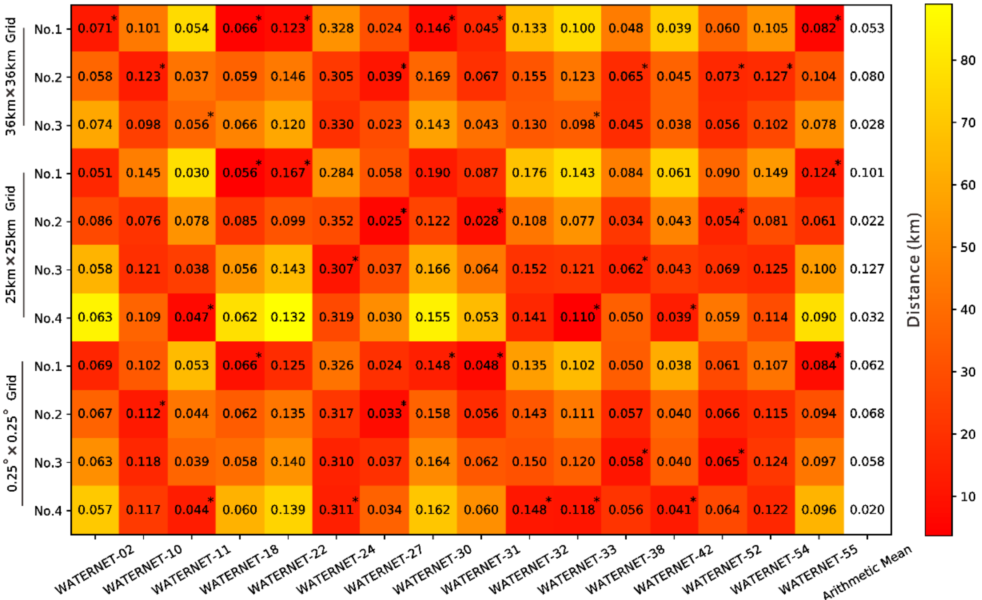
3.1. Obtaining Samples of the Upscaled SM

The MODIS NDVI and LST products are used to establish the LST-NDVI space during the unfrozen season. To obtain comparable TVDI values among different days in a year, it is feasible to plot the annual LST-NDVI scatterplot [57]. To determine the parameters of dry and wet edges, the range of NDVI values (x-axis in Figure 3) is first split into several equal intervals, and then the minimum and maximum LST values in each interval are extracted from the LST-NDVI space. Finally, as shown in Figure 3, $LS{T}_{min}$ is estimated by averaging the minimum LST value in each interval, and $LS{T}_{max}$ is determined by fitting points with maximum LST values. The points located outside dry and wet edges as outliers are not calculated. From 2015 to 2017, the wet edges were almost the same, but the differences among annual dry edges were obvious, and in 2016, there was a maximum dry edge due to the high LST value. By analyzing meteorological data from station A’rou, it was also proven that the near-surface mean air temperature in the unfrozen season of 2016, with a value of 9.62°C, was higher than those with values of 8.21°C and 8.98° in 2015 and 2017, respectively.

Based on the estimated dry and wet edges, the daily TVDI values were calculated according to Equation (6). Figure 4 shows the spatial distribution of the TVDI over several days. Due to cloud cover, the TVDI data had a mass of missing pixels, but the spatiotemporal changes in the dry and wet conditions of soil could be captured. There were significant seasonal variations in the TVDI data from May to September each year. The dry index was higher on the lowland area around the Babao River from northwest to southeast than that in the mountains and was lower on the south slope than on the north slope, indicating that the spatial distribution of the TVDI was in accordance with that of the SM in the Babao River basin, as described in Section 2.1. The SM observations from the 16 upscaled EHWSN nodes were used to build relationships with the TVDI values at the pixels spatially corresponding to ground-based sites. As shown in Figure 5, a monotonically decreasing linear function was fitted according to Equation (7), showing a goodness of determination coefficient indicating the high correlation between the TVDI and SM. Then, the linear regression model was used to transform the TVDI into samples of the upscaled SM.

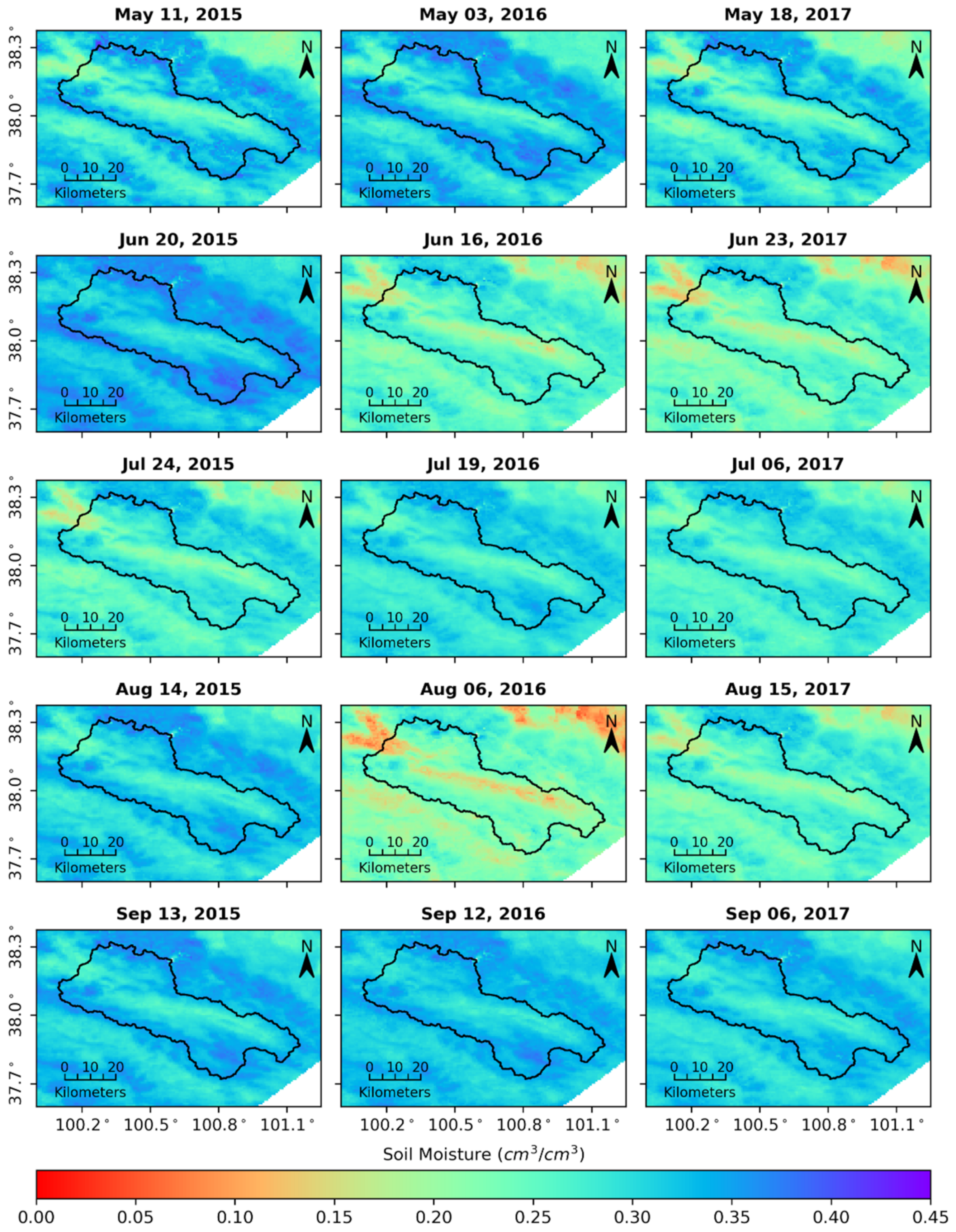
3.2. Upscaling Ground-Based SM Observations

The TVDI-based SM as samples can describe the temporal variability of soil moisture at the $pth$ upscaled pixel to solve Equation (4) for the weighted coefficient vector ${\beta }^p$, and then the upscaled SM can be estimated as a linear combination of the EHWSN observations based on Equation (5). The daily upscaled SM maps, with a spatial resolution of 1 km, are shown in Figure 6, and compared with the TVDI shown in Figure 4, the spatiotemporal trend of the upscaled results was consistent with that of the TVDI, indicating that the correlation between the ancillary data and SM was the crucial factor affecting the upscaling accuracy. The upscaled results had a detailed spatiotemporal distribution relative to the TVDI. Although the ancillary data had numerous gaps due to cloud cover, the EHWSN observations with temporal continuity could fill the upscaled SM at the missing pixels based on constant weighted coefficients in the upscaling time window. In addition, the upscaled SM process in the Babao River basin from August to September 2013 was performed by Kang et al. [29] using the upscaling method used in this paper. There was a similar spatial trend between the previous results and the upscaled SM in this study, showing higher SM in the mountains than in the wide valleys.

3.3. Validation of the Upscaled SM

Rainfall is a primary factor causing spatiotemporal changes in SM. The accuracy of upscaled SM can be indirectly evaluated by detecting the response of SM to rainfall. In Figure 7, the ground-based SM and rainfall observations from the AMSs, including stations A’rou and Jingyangling, were compared with the upscaled results in terms of the consistency of temporal changes. However, not all rainfall events caused daily SM to increase, and this result was related to the amount of rainfall. According to the AMS observations, 193 rainfall events led to an increase in in situ SM, and 85% of these events harmonized with the changes in the upscaled SM. For rainfall with more than 10 mm, of which there were 57 occurrences, only four rainfall events contradicted the changes in the upscaled SM. For heavy rain events (25.0–49.9 mm) or rainstorms (50.0–99.9 mm), the upscaled SM increased at different levels.

The EHWSN observations with missing data were employed to evaluate the upscaled results (see Figure 8). Due to the spatial scale mismatch between the in situ observations and the upscaled SM, the representativeness error led to the mean and amplitude bias of the upscaled results relative to the point-scale EHWSN observations, and the maximum mean bias reached 0.21 cm³ cm⁻³. Thus, the ubRMSE index was used to improve the performance metric of the upscaled SM. There were no obvious differences among the mean annual ubRMSEs, which had an approximate value of 0.03 cm³ cm⁻³. The R was also an insensitive index to the mean bias and was adopted to evaluate the consistency of the temporal change between the ground-based and upscaled SM values. As shown in

Table 2. Validation of the upscaled SM.

Year	2015		2016		2017
Station	R	ubRMSE	R	ubRMSE	R	ubRMSE
WSN-01	0.883	0.028	——	——	——	——
WSN-04	0.654	0.042	0.919	0.026	——	——
WSN-05	0.630	0.056	0.616	0.060	——	——
WSN-06	0.920	0.012	0.668	0.041	0.644	0.053
WSN-12	0.622	0.036	0.794	0.029	——	——
WSN-16	——	——	0.692	0.025	0.864	0.008
WSN-25	0.794	0.018	0.845	0.020	0.793	0.024
WSN-35	0.535	0.057	0.875	0.010	0.652	0.047
WSN-36	——	——	0.880	0.030	——	——
WSN-37	0.493	0.029	0.259	0.038	——	——
WSN-40	0.865	0.017	0.724	0.026	0.887	0.027

The darker the color, the larger the statistical value is.

, overall, the larger the correlation coefficient was, the smaller the ubRMSE value. The averaged R index was 0.73, representing a high correlation. Only the WSN-37 observations, where soil was dry, had a low correlation with the upscaled SM because of the low representativeness of ground-based observations in terms of amplitude change.

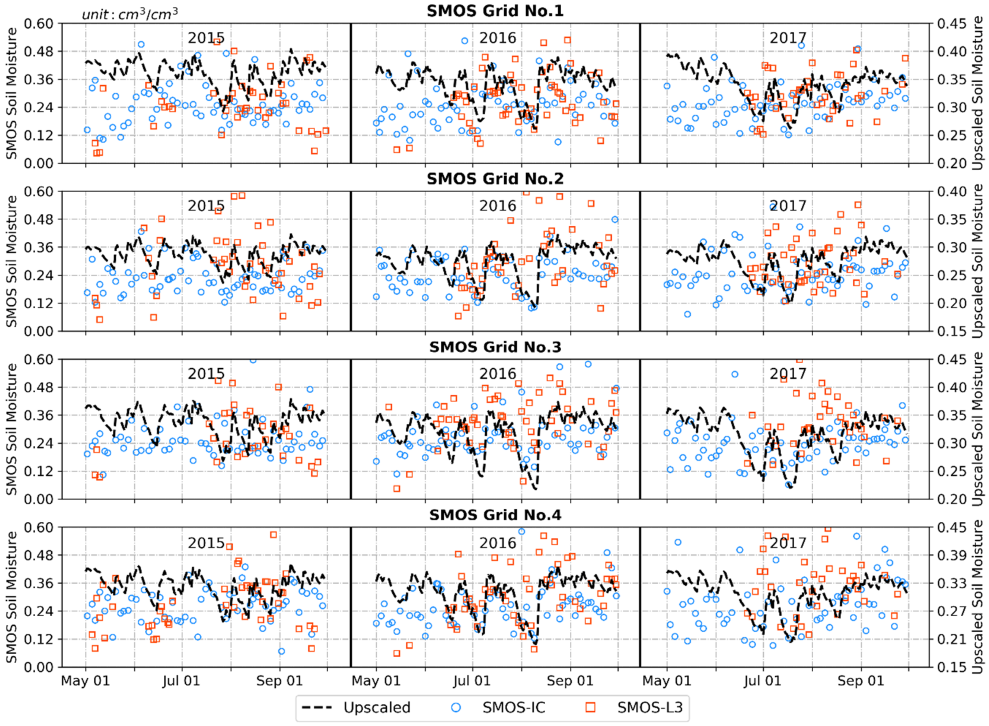
3.4. Comparisons between the Upscaled SM and Microwave Remotely Sensed SM Products

Generally, ground-based SM observations are considered reliable reference data to evaluate RS SM products. However, the point and RS observations were spatially mismatched, but this problem could be solved by upscaling multipoint observations. In this paper, the upscaled SM with a spatial resolution of 1 km could meet the validation requirement of RS SM products at different spatial scales, and the process was performed by resampling the upscaled SM values to match the spatial resolutions of the RS SM products.

As shown in Figure 9, SMAP products including SMAP_L3_SM_P and SMAP_L3_SM_P_E (the SMAP_L3_SM_P_E product was first aggregated to 36 km) were compared with the upscaled SM at the spatial scale of 36 km. The accuracies of both SMAP products on the ubRMSE and R indexes were almost the same, with average statistical values of 0.028 cm³ cm⁻³ and 0.610, respectively. The difference in their accuracy values was mainly reflected in the bias index, indicating that the SMAP_L3_SM_P and SMAP_L3_SM_P_E products were underestimated by 0.066 cm³ cm⁻³ and 0.054 cm³ cm⁻³ (see

Table 3. Performance metrics of RS SM products.

Year	2015				2016				2017
Index	RMSE	ubRMSE	Bias	r	RMSE	ubRMSE	Bias	r	RMSE	ubRMSE	Bias	r
Grid	SMAP_L3_SM_P
No.1	0.097	0.023	−0.095	0.519	0.085	0.026	−0.081	0.710	0.073	0.026	−0.068	0.641
No.2	0.132	0.019	−0.130	0.556	0.117	0.025	−0.115	0.728	0.110	0.023	−0.108	0.677
No.3	0.040	0.038	−0.014	0.363	0.033	0.033	0.002	0.715	0.038	0.036	0.011	0.579
Grid	SMAP_L3_SM_P_E
No.1	0.075	0.025	−0.070	0.501	0.063	0.028	−0.056	0.709	0.054	0.028	−0.046	0.619
No.2	0.115	0.021	−0.113	0.487	0.100	0.024	−0.097	0.752	0.094	0.024	−0.090	0.669
No.3	0.040	0.036	−0.016	0.375	0.031	0.031	−0.003	0.723	0.035	0.034	0.007	0.609
Grid	SMOS_IC
No.1	0.119	0.077	−0.091	0.356	0.114	0.080	−0.081	0.311	0.102	0.078	−0.065	0.269
No.2	0.079	0.060	−0.050	0.475	0.068	0.063	−0.024	0.611	0.089	0.087	−0.021	0.234
No.3	0.112	0.086	−0.072	0.045	0.098	0.090	−0.040	0.277	0.104	0.074	−0.073	0.413
No.4	0.094	0.077	−0.054	0.089	0.093	0.086	−0.037	0.294	0.105	0.102	−0.026	0.343
Grid	SMOS_L3
No.1	0.136	0.105	−0.087	0.033	0.109	0.094	−0.056	0.349	0.085	0.081	−0.026	0.371
No.2	0.129	0.128	0.020	0.033	0.125	0.123	0.022	0.201	0.101	0.098	0.027	0.155
No.3	0.121	0.115	−0.038	−0.214	0.094	0.090	0.026	0.272	0.114	0.112	0.020	-0.116
No.4	0.123	0.120	−0.026	−0.217	0.093	0.092	0.016	0.565	0.134	0.121	0.058	0.108
Grid	AMSR2_JAXA
No.1	0.095	0.075	0.058	−0.026	0.113	0.076	0.084	0.097	0.093	0.072	0.059	0.109
No.2	0.090	0.076	0.047	0.053	0.112	0.075	0.083	0.130	0.086	0.067	0.053	0.070
No.3	0.097	0.075	0.062	0.013	0.132	0.091	0.096	−0.036	0.093	0.067	0.065	0.079
No.4	0.119	0.071	0.095	0.206	0.143	0.078	0.120	0.014	0.115	0.060	0.098	0.100
Grid	AMSR2_NASA_X
No.1	0.140	0.089	0.107	0.384	0.141	0.084	0.113	0.674	0.151	0.096	0.116	0.488
No.2	0.121	0.090	0.081	0.460	0.125	0.090	0.087	0.675	0.139	0.090	0.105	0.384
No.3	0.138	0.082	0.110	0.417	0.135	0.088	0.102	0.575	0.134	0.075	0.111	0.553
No.4	0.137	0.080	0.111	0.436	0.144	0.085	0.115	0.622	0.147	0.077	0.125	0.500
Grid	CCI_SM_v4.7
No.1	0.119	0.035	−0.113	0.579	0.088	0.039	−0.079	0.700	0.095	0.046	−0.084	0.515
No.2	0.102	0.029	−0.098	0.598	0.074	0.035	−0.066	0.767	0.072	0.042	−0.058	0.493
No.3	0.106	0.035	−0.100	0.574	0.080	0.035	−0.072	0.777	0.085	0.041	−0.074	0.632
No.4	0.098	0.036	−0.091	0.498	0.072	0.036	−0.062	0.774	0.078	0.043	−0.065	0.579
Grid	CCI_SM_v5.2
No.1	0.111	0.028	−0.108	0.548	0.084	0.035	−0.077	0.683	0.085	0.039	−0.075	0.560
No.2	0.089	0.034	−0.082	0.472	0.065	0.036	−0.054	0.705	0.059	0.040	−0.043	0.552
No.3	0.108	0.035	−0.103	0.456	0.078	0.031	−0.072	0.783	0.087	0.038	−0.078	0.634
No.4	0.094	0.037	−0.087	0.399	0.066	0.034	−0.057	0.764	0.070	0.040	−0.058	0.641

The darker the color, the larger the statistical value is.

), respectively. The larger underestimation occurred in May and June because the modeled surface temperature showing obviously seasonal changes with low values in the same months was adopted in the SMAP SM retrieval. As a whole, the disaggregated SMAP_L3_SM_P_E product preserved the original brightness temperature used in the retrieval of the SMAP_L3_SM_P product. Thus, both SMAP products had similar accuracies, which was also proven using ground-based observation networks at the global scale in the study of Chan et al. [58].

Like SMAP, SMOS carrying sensors with the same observation band (L-band) have attracted increasing attention due to their better capacity to penetrate vegetation canopies. In the study area, as shown in Figure 10, the SMOS-L3 and SMOS-IC products did not yield similar skills to the SMAP, especially in terms of the R indexes, which showed low consistencies between the upscaled SM and SMOS products and had values of 0.310 for SMOS-IC and 0.128 for SMOS-L3. The SMOS products had a mean anomaly bias of 0.093 cm³ cm⁻³ represented by the ubRMSE index, which was approximately three times that of the SMAP products. The mean biases of the SMOS products, with -0.053 cm³ cm⁻³ for SMOS-IC and -0.004 cm³ cm⁻³ for SMOS-L3, were smaller than those of the SMAP products. The SMOS-IC product had a retrieval algorithm similar to that of SMOS-L3, but several simplifications, such as rejecting some ancillary data, were implemented. Compared with SMOS-L3, the accuracy of SMOS-IC on the RMSE index was not obviously improved. However, the averaged anomaly accuracies of SMOS-IC on the R and ubRMSE indexes were higher than those of SMOS-L3, and the R values still represented a weak correlation.

The AMSR2 products have obvious overestimation relative to the upscaled SM in terms of bias, with a value of 0.077 cm³ cm⁻³ for AMSR2_JAXA and 0.107 cm³ cm⁻³ for AMSR2_NASA_X. Compared with AMSR2_NASA_X with an ubRMSE of 0.086 cm³ cm⁻³, the AMSR2_JAXA product showed a smaller temporal fluctuation range with a lower ubRMSE of 0.074 cm³ cm⁻³ (see Figure 11). Due to the larger bias and ubRMSE values, the total error of AMSR2_NASA_X, with an averaged RMSE value of 0.137 cm³ cm⁻³, exceeded that of AMSR2_JAXA, with an averaged RMSE value of 0.107 cm³ cm⁻³. However, with regard to describing the temporal trend of the upscaled SM, AMSR2_NASA_X, with an averaged R value of 0.514, it was superior to AMSR2_JAXA, with an averaged R value of 0.067, meaning that AMSR2_NASA_X had stronger applicability than AMSR2_JAXA in the study area due to its better consistency with the SM signal. In addition, the R value of AMSR2_NASA_X was higher than that of SMOS, which deviates from the theoretical fact that the L-band is more sensitive to SM than the X-band. It is possible that the underlying surface in this study area is beneficial to LPRM SM retrievals. This phenomenon has also occurred in other validation activities, e.g., in Yee et al. [59] and Ma et al. [60].

Through the above analysis, RS SM products with different observation bands and retrieval algorithms showed various performances, and a single product did not always have the best performance on different evaluation indexes. The CCI SM product merging multiple single RS SM datasets was shown to improve the accuracy of satellite-based SM. In this paper, the CCI SM combining active and passive SM products, with two different versions, were compared, as shown in Figure 12. Compared with SMAP with better skills based on the above analysis, the performance of the CCI showed a slightly higher mean R value of 0.612. For other performance metrics of the CCI, including an average RMSE of 0.086 cm³ cm⁻³, an average ubRMSE of 0.037 cm³ cm⁻³ and an average bias of -0.077 cm³ cm⁻³, the accuracies of the CCI were inferior to those of SMAP. The accuracy differences between the CCI SM products version 4.7 and 5.2 were not obvious because all RS SM products merged into different versions of CCI products were rescaled based on the same SM simulation dataset. Therefore, although the SMAP SM was introduced into the latest version of the CCI SM, the accuracy of the CCI had not been significantly changed due to attenuated satellite observation features in the rescaling process.

4. Discussion

The accuracy of the upscaled SM is affected by both sides including the representative SM that is the sample of the upscaled SM and the performance of the upscaling algorithm. The sample decides the spatio-temporal trend of the upscaled SM, thus an ancillary data highly related to SM is needed. The ATI and SEE are also recognized as the ancillary data to monitor the spatio-temporal variability of SM besides the TVDI. However, in current studies, the correlations between SM and these three variables are not compared with each other. The sample obtained by transforming any ancillary data may have system bias and random error and can be applied in the upscaling processing when there is no system error. Kang et al. [30] have proven that the sample has the low mean and amplitude bias in this study area but random error still exists. To reduce the influence of random error on the upscaled SM, an upscaling algorithm with good prediction performance should be employed. Though the traditional ordinary least square (OLS) regression method can build the relationship of the ground-based observation and the upscaled SM, random error is also fitted leading to the regression model with poor prediction (overfitting). In this study, the upscaling method introduces a regularization parameter to solve the overfitting problem. Kang et al. [43] found that the introduction of the regularization parameter could reduce the uncertainty of the upscaled SM.

The necessity to upscale ground-based observations is a matter of concern in this study. The single-point and multi-point arithmetic average validation are commonly used to assess SM retrieval values at their corresponding pixels. However, the representativeness of ground-based observations to the truth at the pixel scale are generally neglected due to the unknown truth. In this study, the representative error of ground-based observations can be estimated when the upscaled SM at difference scales is considered the relative truth. As shown in Figure 13, the RMSE index is used to measure the representative error, whose maximum and mean reach more than 0.300 cm³ cm⁻³ and 0.092 cm³ cm⁻³, respectively, meaning that the single-point validation is unreliable. In addition, for a certain pixel, the most representative site may not locate within the pixel zone but rather away from the pixel. Therefore, it is justified that the upscaling algorithm in this study employs all ground-based observations for each upscaled pixel.

The multi-point average value is closer to the relative truth than the single-point observation, but the representative error having an averaged RMSE of 0.059 cm³ cm⁻³ still needs to be considered. Due to different representativeness of sites, the representative error of the multi-point arithmetic mean does not always reduce with the increase of the number of sites, e.g., 4-site average with a RMSE value of 0.028 cm³ cm⁻³ for Grid No.3 of 36 km and 2-site average with a RMSE value of 0.053 cm³ cm⁻³ for Grid No.1 of 36 km, indicating that the assignation of equal weight coefficients to sites is not the optimal scheme, especially when the spatial distribution of ground-based sites within a pixel zone is sparse. The upscaling algorithm can give the weighted average of ground-based observations for the upscaled SM at each pixel showing an obvious advantage on upscaling sparse ground-based observations.

5. Conclusions

Ground-based observations are considered reliable reference data in the validation activities of RS products. For microwave RS SM products, however, the spatial distribution of ground-based sites generally shows a low density relative to the RS SM pixel (25–40 km), and the mismatched scale between point and RS observations may cause representativeness errors in the performance metrics. To better understand the accuracies of microwave RS SM products, a temporal upscaling algorithm was employed to transform sparse point-scale observations into pixel-scale values. In the upscaling process, the TVDI, which is strongly related to SM, was introduced to capture the spatial heterogeneity of SM. The upscaled SM with a 1 km resolution in the study area was first evaluated using in situ SM measurements and showed high performance in terms of temporal consistency and amplitude accuracy. Approximately 85% of rainfall events could be captured by the upscaled SM. Compared with previous research in the same study area, the upscaled SM in this paper had a similar spatial trend. Therefore, it was feasible to obtain the reference data using the upscaling algorithm in this study. Finally, the upscaled SM with 1 km resolution was regarded as reference data to validate RS SM products at the same spatial scale.

To meet the validation requirement at different spatial scales, the high resolution of the upscaled SM was resampled to match the spatial scales of various RS SM products. In the study area, the L-band and combined CCI SM were significantly underestimated, but the AMSR2 SM was overestimated. In addition to the R value of the CCI being slightly higher than that of SMAP, the performance of SMAP was the best of all validated RS SM products, followed by that of CCI, AMSR2_NASA_X, SMOS-IC, SMOS-L3, and AMSR2_JAXA. The accuracy of SMOS did not reach the theoretical expectation in this study, although the retrieval algorithm was developed for SMOS. SMAP and CCI had better performance, but they still could not meet the application requirement for an accuracy of less than 0.04 cm³ cm⁻³.

This validation result is applicable only in this study area and cannot answer the whole accuracy of an RS SM product; however, the regional validation results can explain the error characteristic under some underlying surfaces. To understand the global accuracy, an RS SM product was considered as reference data used to evaluate other values in previous research, but this approach is risky because no single RS SM product always has the best performance at different spatial pixels, a result proven in this and previous studies. Thus, a pixel-by-pixel validation scheme is urgently needed to accurately understand the overall accuracies of RS SM products to promote their applications in various fields.

References

1. GCOS. Implementation plan for the global observing system for climate in support of the UNFCCC (2010 Update). In Proceedings of the Conference of the Parties (COP), Copenhagen, Denmark, 7–18 December 2010. [Google Scholar]
2. Brocca, L.; Melone, F.; Moramarco, T.; Wagner, W.; Naeimi, V.; Bartalis, Z.; Hasenauer, S. Improving runoff prediction through the assimilation of the ASCAT soil moisture product. Hydrol. Earth Syst. Sci. 2010, 14, 1881. [Google Scholar] [CrossRef] [Green Version]
3. Massari, C.; Brocca, L.; Moramarco, T.; Tramblay, Y.; Lescot, J.-F.D. Potential of soil moisture observations in flood modelling: Estimating initial conditions and correcting rainfall. Adv. Water Res. 2014, 74, 44–53. [Google Scholar] [CrossRef]
4. Hunt, K.M.R.; Turner, A.G. The effect of soil moisture perturbations on indian monsoon depressions in a numerical weather prediction model. J. Clim. 2017, 30, 8811–8823. [Google Scholar] [CrossRef]
5. Dharssi, I.; Bovis, K.J.; Macpherson, B.; Jones, C.P. Operational assimilation of ASCAT surface soil wetness at the met office. Hydrol. Earth Syst. Sci. 2011, 15, 2729–2746. [Google Scholar] [CrossRef] [Green Version]
6. McNairn, H.; Merzouki, A.; Pacheco, A.; Fitzmaurice, J. Monitoring soil moisture to support risk reduction for the agriculture sector using radarsat-2. IEEE J. Sel. Top. Appl. Earth Obs. Remote Sens. 2012, 5, 824–834. [Google Scholar] [CrossRef]
7. Bolten, J.D.; Crow, W.T.; Zhan, X.; Jackson, T.J.; Reynolds, C.A. Evaluating the utility of remotely sensed soil moisture retrievals for operational agricultural drought monitoring. IEEE J. Sel. Top. Appl. Earth Obs. Remote Sens. 2009, 3, 57–66. [Google Scholar] [CrossRef] [Green Version]
8. Miralles, D.G.; Holmes, T.R.H.; De Jeu, R.A.M.; Gash, J.H.; Meesters, A.G.C.A.; Dolman, A.J. Global land-surface evaporation estimated from satellite-based observations. Hydrol. Earth Syst. Sci. 2011, 15, 453–469. [Google Scholar] [CrossRef] [Green Version]
9. Seneviratne, S.I.; Corti, T.; Davin, E.L.; Hirschi, M.; Jaeger, E.B.; Lehner, I.; Orlowsky, B.; Teuling, A.J. Investigating soil moisture–climate interactions in a changing climate: A review. Earth Sci. Rev. 2010, 99, 125–161. [Google Scholar] [CrossRef]
10. Liu, Y.Y.; Dorigo, W.A.; Parinussa, R.M.; de Jeu, R.A.M.; Wagner, W.; McCabe, M.F.; Evans, J.P.; van Dijk, A.I.J.M. Trend-preserving blending of passive and active microwave soil moisture retrievals. Remote Sens. Environ. 2012, 123, 280–297. [Google Scholar] [CrossRef]
11. Justice, C.; Belward, A.; Morisette, J.; Lewis, P.; Privette, J.; Baret, F. Developments in the ‘validation’ of satellite sensor products for the study of the land surface. Int. J. Remote Sens. 2000, 21, 3383–3390. [Google Scholar] [CrossRef]
12. Verstraeten, W.W.; Veroustraete, F.; van der Sande, C.J.; Grootaers, I.; Feyen, J. Soil moisture retrieval using thermal inertia, determined with visible and thermal spaceborne data, validated for European forests. Remote Sens. Environ. 2006, 101, 299–314. [Google Scholar] [CrossRef]
13. Merlin, O.; Walker, J.P.; Chehbouni, A.; Kerr, Y. Towards deterministic downscaling of SMOS soil moisture using MODIS derived soil evaporative efficiency. Remote Sens. Environ. 2008, 112, 3935–3946. [Google Scholar] [CrossRef] [Green Version]
14. Clewley, D.; Whitcomb, J.; Akbar, R.; Silva, A.; Berg, A.; Adams, J.; Caldwell, T.; Entekhabi, D.; Moghaddam, M. A method for upscaling in situ soil moisture measurements to satellite footprint scale using random forests. IEEE J. Sel. Top. Appl. Earth Obs. Remote Sens. 2017, 10, 2663–2673. [Google Scholar] [CrossRef]
15. Reichle, R.H.; Koster, R.D. Bias reduction in short records of satellite soil moisture. Geophys. Res. Lett. 2004, 31. [Google Scholar] [CrossRef] [Green Version]
16. Albergel, C.; Dutra, E.; Munier, S.; Calvet, J.C.; Munoz-Sabater, J.; de Rosnay, P.; Balsamo, G. Era-5 and era-interim driven isba land surface model simulations: Which one performs better? Hydrol. Earth Syst. Sci. 2018, 22, 3515–3532. [Google Scholar] [CrossRef] [Green Version]
17. Rodell, M.; Houser, P.; Jambor, U.E.A.; Gottschalck, J.; Mitchell, K.; Meng, J.; Arsenault, K.; Brian, C.; Radakovich, J.; Mg, B.; et al. The global land data assimilation system. Bull. Am. Meteorol. Soc. 2004, 85, 381–394. [Google Scholar] [CrossRef] [Green Version]
18. Al-Yaari, A.; Wigneron, J.-P.; Ducharne, A.; Kerr, Y.; Wagner, W.; De Lannoy, G.; Reichle, R.; Al Bitar, A.; Dorigo, W.; Richaume, P. Global-scale comparison of passive (SMOS) and active (ASCAT) satellite based microwave soil moisture retrievals with soil moisture simulations (MERRA-Land). Remote Sens. Environ. 2014, 152, 614–626. [Google Scholar] [CrossRef] [Green Version]
19. Al-Yaari, A.; Wigneron, J.P.; Ducharne, A.; Kerr, Y.; de Rosnay, P.; de Jeu, R.; Govind, A.; Al Bitar, A.; Albergel, C.; Muñoz-Sabater, J.; et al. Global-scale evaluation of two satellite-based passive microwave soil moisture datasets (SMOS and AMSR-E) with respect to land data assimilation system estimates. Remote Sens. Environ. 2014, 149, 181–195. [Google Scholar] [CrossRef] [Green Version]
20. Fang, L.; Hain, C.R.; Zhan, X.; Anderson, M.C. An inter-comparison of soil moisture data products from satellite remote sensing and a land surface model. Int. J. Appl. Earth Obs. Geoinf. 2016, 48, 37–50. [Google Scholar] [CrossRef]
21. Nykanen, D.K.; Foufoula-Georgiou, E. Soil moisture variability and scale-dependency of nonlinear parameterizations in coupled land–atmosphere models. Adv. Water Res. 2001, 24, 1143–1157. [Google Scholar] [CrossRef]
22. Burgin, M.S.; Colliander, A.; Njoku, E.G.; Chan, S.K.; Cabot, F.; Kerr, Y.H.; Bindlish, R.; Jackson, T.J.; Entekhabi, D.; Yueh, S.H. A comparative study of the SMAP passive soil moisture product with existing satellite-based soil moisture products. IEEE Trans. Geosci. Remote Sens. 2017, 55, 2959–2971. [Google Scholar] [CrossRef] [PubMed]
23. Tugrul Yilmaz, M.; Crow, W. Evaluation of assumptions in soil moisture triple collocation analysis. J. Hydrometeorol. 2014, 15, 1293–1302. [Google Scholar] [CrossRef]
24. McColl, K.A.; Vogelzang, J.; Konings, A.G.; Entekhabi, D.; Piles, M.; Stoffelen, A. Extended triple collocation: Estimating errors and correlation coefficients with respect to an unknown target. Geophys. Res. Lett. 2014, 41, 6229–6236. [Google Scholar] [CrossRef] [Green Version]
25. Gruber, A.; Su, C.H.; Zwieback, S.; Crow, W.; Dorigo, W.; Wagner, W. Recent advances in (soil moisture) triple collocation analysis. Int. J. Appl. Earth Obs. Geoinf. 2016, 45, 200–211. [Google Scholar] [CrossRef]
26. Draper, C.; Reichle, R.; de Jeu, R.; Naeimi, V.; Parinussa, R.; Wagner, W. Estimating root mean square errors in remotely sensed soil moisture over continental scale domains. Remote Sens. Environ. 2013, 137, 288–298. [Google Scholar] [CrossRef] [Green Version]
27. Dorigo, W.; Scipal, K.; Parinussa, R.; Liu, Y.; Wagner, W.; De Jeu, R.; Naeimi, V. Error characterisation of global active and passive microwave soil moisture datasets. Hydrol. Earth Syst. Sci. 2010, 14, 2605–2616. [Google Scholar] [CrossRef] [Green Version]
28. Gruber, A.; Su, C.H.; Crow, W.T.; Zwieback, S.; Dorigo, W.A.; Wagner, W. Estimating error cross-correlations in soil moisture data sets using extended collocation analysis. J. Geophys. Res. Atmos. 2016, 121, 1208–1219. [Google Scholar] [CrossRef] [Green Version]
29. Kang, J.; Jin, R.; Li, X.; Ma, C.; Qin, J.; Zhang, Y. High spatio-temporal resolution mapping of soil moisture by integrating wireless sensor network observations and modis apparent thermal inertia in the babao river basin, China. Remote Sens. Environ. 2017, 191, 232–245. [Google Scholar] [CrossRef] [Green Version]
30. Kang, J.; Jin, R.; Li, X.; Zhang, Y. Error decomposition of remote sensing soil moisture products based on the triple-collocation method introducing an unbiased reference dataset: A case study on the tibetan plateau. Remote Sens. 2020, 12, 3087. [Google Scholar] [CrossRef]
31. Dorigo, W.; Wagner, W.; Hohensinn, R.; Hahn, S.; Paulik, C.; Xaver, A.; Gruber, A.; Drusch, M.; Mecklenburg, S.; Oevelen, P.V. The international soil moisture network: A data hosting facility for global in situ soil moisture measurements. Hydrol. Earth Syst. Sci. 2011, 15, 1675–1698. [Google Scholar] [CrossRef] [Green Version]
32. Bell, J.E.; Palecki, M.A.; Baker, C.B.; Collins, W.G.; Lawrimore, J.H.; Leeper, R.D.; Hall, M.E.; Kochendorfer, J.; Meyers, T.P.; Wilson, T.; et al. U.S. Climate reference network soil moisture and temperature observations. J. Hydrometeorol. 2013, 14, 977–988. [Google Scholar] [CrossRef]
33. Smith, A.B.; Walker, J.P.; Western, A.W.; Young, R.I.; Ellett, K.M.; Pipunic, R.C.; Grayson, R.B.; Siriwardena, L.; Chiew, F.H.S.; Richter, H. The murrumbidgee soil moisture monitoring network data set. Water Resour. Res. 2012, 48, 1–6. [Google Scholar] [CrossRef]
34. Tagesson, T.; Fensholt, R.; Guiro, I.; Rasmussen, M.O.; Huber, S.; Mbow, C.; Garcia, M.; Horion, S.; Sandholt, I.; Holm-Rasmussen, B.; et al. Ecosystem properties of semiarid savanna grassland in west Africa and its relationship with environmental variability. Glob. Chang. Biol. 2015, 21, 250–264. [Google Scholar] [CrossRef] [Green Version]
35. Zacharias, S.; Bogena, H.; Samaniego, L.; Mauder, M.; Fuß, R.; Pütz, T.; Frenzel, M.; Schwank, M.; Baessler, C.; Butterbach-Bahl, K.; et al. A network of terrestrial environmental observatories in Germany. Vadose Zone J. 2011, 10, 955–973. [Google Scholar] [CrossRef] [Green Version]
36. Calvet, J.; Fritz, N.; Froissard, F.; Suquia, D.; Petitpa, A.; Piguet, B. In situ soil moisture observations for the CAL/VAL of SMOS: The smosmania network. In Proceedings of the 2007 IEEE International Geoscience and Remote Sensing Symposium, Barcelona, Spain, 23–28 July 2007; pp. 1196–1199. [Google Scholar]
37. Su, Z.; Wen, J.; Dente, L.; Velde, R.; Wang, L.; Ma, Y.; Yang, K.; Hu, Z. The Tibetan plateau observatory of plateau scale soil moisture and soil temperature (Tibet-Obs) for quantifying uncertainties in coarse resolution satellite and model products. Hydrol. Earth Syst. Sci. 2011, 15, 2303–2316. [Google Scholar] [CrossRef] [Green Version]
38. Gruber, A.; Dorigo, W.A.; Zwieback, S.; Xaver, A.; Wagner, W. Characterizing coarse-scale representativeness of in situ soil moisture measurements from the international soil moisture network. Vadose Zone J. 2013, 12, vzj2012.0170. [Google Scholar] [CrossRef] [Green Version]
39. De Rosnay, P.; Gruhier, C.; Timouk, F.; Baup, F.; Mougin, E.; Hiernaux, P.; Kergoat, L.; LeDantec, V. Multi-scale soil moisture measurements at the Gourma meso-scale site in Mali. J. Hydrol. 2009, 375, 241–252. [Google Scholar] [CrossRef] [Green Version]
40. Gruhier, C.; de Rosnay, P.; Hasenauer, S.; Holmes, T.; de Jeu, R.; Kerr, Y.; Mougin, E.; Njoku, E.; Timouk, F.; Wagner, W.; et al. Soil moisture active and passive microwave products: Intercomparison and evaluation over a Sahelian site. Hydrol. Earth Syst. Sci. 2010, 14, 141–156. [Google Scholar] [CrossRef] [Green Version]
41. Qin, J.; Yang, K.; Lu, N.; Chen, Y.; Zhao, L.; Han, M. Spatial upscaling of in-situ soil moisture measurements based on Modis-derived apparent thermal inertia. Remote Sens. Environ. 2013, 138, 1–9. [Google Scholar] [CrossRef]
42. Gao, S.; Zhu, Z.; Haiteng, W.; Zhang, J. Upscaling of sparse in situ soil moisture observations by integrating auxiliary information from remote sensing. Int. J. Remote Sens. 2017, 38, 4782–4803. [Google Scholar] [CrossRef]
43. Kang, J.; Jin, R.; Li, X.; Zhang, Y.; Zhu, Z. Spatial upscaling of sparse soil moisture observations based on ridge regression. Remote Sens. 2018, 10, 192. [Google Scholar] [CrossRef] [Green Version]
44. Jin, R.; Li, X.; Yan, B.; Li, X.; Luo, W.; Ma, M.; Guo, J.; Kang, J.; Zhu, Z.; Zhao, S. A nested ecohydrological wireless sensor network for capturing the surface heterogeneity in the midstream areas of the Heihe river basin, china. Geosci. Remote Sens. Lett. IEEE 2014, 11, 2015–2019. [Google Scholar] [CrossRef]
45. Liu, S.; Li, X.; Xu, Z.; Che, T.; Xiao, Q.; Ma, M.; Liu, Q.; Jin, R.; Guo, J.; Wang, L.; et al. The Heihe integrated observatory network: A basin-scale land surface processes observatory in china. Vadose Zone J. 2018, 17, 180072. [Google Scholar] [CrossRef]
46. O’Neill, P.E.; Chan, S.; Njoku, E.G.; Jackson, T.; Bindlish, R.; Chaubell, J. SMAP L3 Radiometer Global Daily 36 km Ease-Grid Soil Moisture, Version 6; NASA National Snow and Ice Data Center Distributed Active Archive Center: Boulder, CO, USA, 2019. [Google Scholar]
47. O’Neill, P.E.; Chan, S.; Njoku, E.G.; Jackson, T.; Bindlish, R.; Chaubell, J. SMAP Enhanced L3 Radiometer Global Daily 9 km Ease-grid Soil Moisture, Version 3; NASA National Snow and Ice Data Center Distributed Active Archive Center: Boulder, CO, USA, 2019. [Google Scholar]
48. Fujii, H.; Koike, T.; Imaoka, K. Improvement of the Amsr-E algorithm for soil moisture estimation by introducing a fractional vegetation coverage dataset derived from Modis data. J. Remote Sens. Soc. Jpn. 2009, 29, 282–292. [Google Scholar]
49. Owe, M.; de Jeu, R.; Holmes, T. Multisensor historical climatology of satellite-derived global land surface moisture. J. Geophys. Res. Earth Surf. 2008, 113. [Google Scholar] [CrossRef]
50. De Jeu, R.; Owe, M. AMSR2/GCOM-W1 Surface Soil Moisture (LPRM) L3 1 Day 25 km × 25 km Ascending/Descending v001; Goddard Earth Sciences Data and Information Services Center (GES DISC): Greenbelt, MD, USA, 2014. [Google Scholar]
51. Al Bitar, A.; Mialon, A.; Kerr, Y.H.; Cabot, F.; Richaume, P.; Jacquette, E.; Quesney, A.; Mahmoodi, A.; Tarot, S.; Parrens, M.; et al. The global SMOS level 3 daily soil moisture and brightness temperature maps. Earth Syst. Sci. Data 2017, 9, 293–315. [Google Scholar] [CrossRef] [Green Version]
52. Fernandez-Moran, R.; Al-Yaari, A.; Mialon, A.; Mahmoodi, A.; Al Bitar, A.; De Lannoy, G.; Lopez-Baeza, E.; Kerr, Y.; Wigneron, J.-P. SMOS-IC: An alternative SMOS soil moisture and vegetation optical depth product. Remote Sens. 2017, 9, 457. [Google Scholar] [CrossRef] [Green Version]
53. Dorigo, W.; Wagner, W.; Albergel, C.; Albrecht, F.; Balsamo, G.; Brocca, L.; Chung, D.; Ertl, M.; Forkel, M.; Gruber, A.; et al. ESA CCI soil moisture for improved earth system understanding: State-of-the art and future directions. Remote Sens. Environ. 2017, 203, 185–215. [Google Scholar] [CrossRef]
54. Gruber, A.; Scanlon, T.; van der Schalie, R.; Wagner, W.; Dorigo, W. Evolution of the ESA CCI soil moisture climate data records and their underlying merging methodology. Earth Syst. Sci. Data 2019, 11, 717–739. [Google Scholar] [CrossRef] [Green Version]
55. Crow, W.T.; Berg, A.A.; Cosh, M.H.; Loew, A.; Mohanty, B.P.; Panciera, R.; Rosnay, P.; Ryu, D.; Walker, J.P. Upscaling sparse ground-based soil moisture observations for the validation of coarse-resolution satellite soil moisture products. Rev. Geophys. 2012, 50, RG2002. [Google Scholar] [CrossRef] [Green Version]
56. Sandholt, I.; Rasmussen, K.; Andersen, J. A simple interpretation of the surface temperature/vegetation index space for assessment of surface moisture status. Remote Sens. Environ. 2002, 79, 213–224. [Google Scholar] [CrossRef]
57. Holzman, M.E.; Rivas, R.; Bayala, M. Subsurface soil moisture estimation by VI–LST method. Geosci. Remote Sens. Lett. IEEE 2014, 11, 1951–1955. [Google Scholar] [CrossRef]
58. Chan, S.K.; Bindlish, R.; O’Neill, P.; Jackson, T.; Njoku, E.; Dunbar, S.; Chaubell, J.; Piepmeier, J.; Yueh, S.; Entekhabi, D.; et al. Development and assessment of the SMAP enhanced passive soil moisture product. Remote Sens. Environ. 2018, 204, 931–941. [Google Scholar] [CrossRef] [PubMed] [Green Version]
59. Yee, M.S.; Walker, J.P.; Rüdiger, C.; Parinussa, R.M.; Koike, T.; Kerr, Y.H. A comparison of smos and amsr2 soil moisture using representative sites of the OZNET monitoring network. Remote Sens. Environ. 2017, 195, 297–312. [Google Scholar] [CrossRef]
60. Ma, H.; Zeng, J.; Chen, N.; Zhang, X.; Cosh, M.H.; Wang, W. Satellite surface soil moisture from SMAP, SMOS, amsr2 and ESA CCI: A comprehensive assessment using global ground-based observations. Remote Sens. Environ. 2019, 231, 111215. [Google Scholar] [CrossRef]
Figure 1. Map of study area.
Remotesensing 13 00228 g001
Figure 2. Definition of the temperature vegetation dryness index (TVDI) [56].
Remotesensing 13 00228 g002
Figure 3. TVDI scatterplot in each year.
Remotesensing 13 00228 g003
Figure 4. Spatiotemporal distribution of the TVDI.
Remotesensing 13 00228 g004
Figure 5. Relationship models between the TVDI and in situ SM. The blue lines represent the 95% confidence intervals of scatter points in the y-axis direction.
Remotesensing 13 00228 g005
Figure 6. Daily upscaled results at the 1 km scale.
Remotesensing 13 00228 g006
Figure 7. Comparison between the AMS (automatic meteorological station) observations and the upscaled SM.
Remotesensing 13 00228 g007
Figure 8. Scatterplots of the Ecological and Hydrological Wireless Sensor Network (EHWSN) observations and the upscaled SM.
Remotesensing 13 00228 g008
Figure 9. Temporal comparisons between the upscaled SM and SMAP products at the 36 km scale.
Remotesensing 13 00228 g009
Figure 10. Temporal comparisons between the upscaled SM and SMOS products at the 25 km scale.
Remotesensing 13 00228 g010
Figure 11. Temporal comparisons between the upscaled SM and ARMS2 products with different retrieval algorithms at the 0.25° scale.
Remotesensing 13 00228 g011
Figure 12. Temporal comparisons between the upscaled SM and CCI products with different versions at the 0.25° scale.
Remotesensing 13 00228 g012
Figure 13. Root-mean-square errors (RMSEs) between in situ measurements and the upscaled SM at multiple pixel scales. The gradient color represents spatial distances between the ground-based sites and the center points of pixels. The asterisk means that the site locates within the pixel zone. The arithmetic mean values are obtained by averaging the ground-based observations derived from multiple sites within the same pixel area. The RMSEs between arithmetic mean values and their corresponding upscaled SM at different pixel scales are shown in the extreme righthand column.
Remotesensing 13 00228 g013