Abstract
Existing multi-exposure fusion (MEF) algorithms for gray images under low-illumination cannot preserve details in dark and highlighted regions very well, and the fusion image noise is large. To address these problems, an MEF method is proposed. First, the latent low-rank representation (LatLRR) is used on low-dynamic images to generate low-rank parts and saliency parts to reduce noise after fusion. Then, two components are fused separately in Laplace multi-scale space. Two different weight maps are constructed according to features of gray images under low illumination. At the same time, an energy equation is designed to obtain the optimal ratio of different weight factors. An improved guided filtering based on an adaptive regularization factor is proposed to refine the weight maps to maintain spatial consistency and avoid artifacts. Finally, a high dynamic image is obtained by the inverse transform of low-rank part and saliency part. The experimental results show that the proposed method has advantages both in subjective and objective evaluation over state-of-the-art multi-exposure fusion methods for gray images under low-illumination imaging.
1. Introduction
Low-illumination imaging can compensate for problems in information collection in low-illumination environments, thus improving national defense ability. The dynamic range of ordinary charge-coupled device (CCD) sensors is approximately 103, which is much smaller than that of a real scene [1,2]. In addition, images taken in low-light conditions are often of low visibility. In fact, the image quality of gray images under low illumination can be improved by using image enhancement methods [3,4]. However, it is difficult to recover image details that are lost due to dynamic range limitation. Multi-exposure image fusion techniques have been introduced to solve the abovementioned issues.
Multi-exposure fusion (MEF) methods are mainly categorized as tone-mapping based on the inverse camera response function (CRF) in the radiance-domain and transforming fusion coefficients in the spatial-domain [5]. The first method involves CRF computation and tonal image mapping, which is time-consuming and difficult to implement [6,7,8]. Therefore, MEF methods based on pixel-level fusion in the spatial-domain are extensively used currently [9,10,11].
Three main types of solutions exist for MEF methods in the spatial-domain. First, most previous exposure fusion approaches merged multiple exposure source images at the pixel level based on some defined weight measures [12,13,14]. Mertens used image contrast, good exposure and saturation information to calculate the initial weight maps based on the Laplacian pyramid. Three adjustment factors were adopted to control the ratio of weights. This method achieved good fusion effects, however there was a problem of losing brightness and dark details [15]. Other measures were proposed to maintain details in the brightest and darkest regions, and most of them focused on how to build weights: an image reconstruction technique based on the Haar wavelet in the gradient domain [16], weighted guided image filter [17,18], the adaptive weight function [19], weight maps based on gradient information [20], adaptive weights based on the relative intensity between the images and global gradients [21] and structural patch decomposition [22]. Weighted sparse representation and a guided filter in gradient domain were proposed to retain image edges more adequately in gray images [23]. The input images are decomposed by non-subsampled contourlet transform and then different fusion rules are applied for low and high frequency NSCT coefficients. Finally the fused image is obtained by the inverse transform [24], and this method obtained good results. On the whole, the pixel-based image fusion method is simple and easy to implement. The fusion effect is limited in extracting details due to its fixed initial weights, and the weights obtained based on a single pixel are susceptible to noise and easily produce visual artifacts in the fusion image.
Patch-based MEF methods have attracted more attention [25,26]. These methods divide multi-exposure images into different patches. Kede Ma proposed an effective structural patch by decomposing an image patch into three conceptually independent components: signal strength, signal structure, and mean intensity. Then, three components are fused separately [27,28]. Wang utilized a super-pixel segmentation approach to divide images into non-overlapping image patches composed of pixels with similar visual properties [29]. An MEF framework based on low-level image features and image patch structure decomposition was proposed to improve the robustness of ghost removal in a dynamic scene, and preserved more detailed information [30]. Overall, this method mainly pays attention to the block segmentation. However, different patches contain pixels with different color and brightness characteristics. If the same fusion rule is used on these pixels with different characteristics, then the color or detail information tends to be lost.
Recently, the convolutional neural network (CNN) has also been applied to extract exposure-invariant features to generate artifact-free fusion images [31,32]. An MEF algorithm for gray images is proposed based on the decomposition CNN and weighted sparse representation [33]. In general, learning-based approaches have a good effect on ghost suppression in dynamic scenes. However, it is difficult to obtain real high dynamic range (HDR) datasets and better utilization of the CNN for MEF requires the solution of the problems associated with the training dataset, network classification accuracy, and loss function.
Generally, there are fewer multi-exposure fusion methods only for gray images under low illumination. Most MEF algorithms are designed for color images under normal illumination. Although these methods can be used in gray images by preprocessing, but the saturation factor in the method [15] is zero and is without practical significance for gray images. Multi-exposure fusion of gray images under low illumination faces two challenges: images under low illumination have low contrast and relatively large noise resulting in a lower signal-to-noise ratio of the fusion image; and compared with color images, gray images have less information available for building fusion weight maps resulting in detail loss in the dark and highlighted regions.
Given these problems, a novel approach based on latent low-rank representation (LatLRR) and adaptive weights is proposed. Moreover, an improved guided filter is used to refine the weight maps to reduce artifacts. The proposed algorithm makes the following contributions:
- (1)
- Before constructing multi-scale Laplace fusion space, LatLRR is utilized to decompose low dynamic range (LDR) images, which is more effective in reducing noise. The global and local structures are treated separately in the multi-scale space.
- (2)
- According to characteristics of gray images under low-light imaging, adaptive weight factors are constructed for the decomposed global and local structures to avoid detail loss in low dark areas and highlighted areas.
- (3)
- An energy function is formulated to obtain the optimal ratio of contrast and exposure scale factors to obtain better robustness.
- (4)
- An improved guided filtering algorithm based on an adaptive regularization factor is proposed to refine the weight maps to maintain spatial consistency and avoid artifacts.
The remainder of this paper is organized as follows: relevant technical background is briefly reviewed in Section 2. In Section 3, the proposed multi-exposure image fusion method is introduced in detail. The experimental results and analysis are shown in Section 4. The conclusions are presented in Section 5.
2. Related Work
2.1. Latent Low-Rank Representation
The latent low-rank representation decomposes the image into a global structure (low-rank representation), a local structure (salient features) and sparse noise [34], and it is robust against noise. The LatLRR decomposition can be defined as follows:
where, is the equilibrium factor, denotes the nuclear norm and is the . is an image with the size of . Z is the low-rank coefficient, L is the saliency coefficient and E is the sparse noise. Then the low-rank representation part XZ(), saliency part LX () and sparse noise part E can be derived. The noise is removed and only the low-rank and saliency parts are performed in fusion processing.
2.2. Guided Filter
The guided filter is an edge-preserving smoothing filter proposed by He et al. [18] and is defined as a linear model using a guidance image X:
where and are the pixel value of the output and guidance image, respectively. and are linear coefficients in a local window with a size of centered on pixel . The coefficients and can directly be estimated using:
where is the original image, and represent the mean and variance of guidance image in local window , respectively. A fixed regularization factor was applied to different local regions in [18], and the difference in image texture between different regions is not taken into consideration. This leads to over-smooth or under-smooth effects. In reality, a smaller is required for regions with rich edge information to sharpen and highlight the edges. By contrast, a larger is required for flat regions to produce a stronger smoothing effect.
3. Proposed Multi-Exposure Fusion Method
In this section, an adaptive MEF method based on digital time delay integration (TDI) images with multiple integral series is presented to promote the application of multi-exposure fusion technology in the field of remote sensing under low-light imaging. Figure 1 shows the framework of the proposed method. First, K images with different integral series are selected and used as multi-exposure images. Second, the image is divided into a low-rank representation part and saliency part using the LatLRR method. Third, for decomposed images, different fusion weight maps are designed according to the characteristics of low-illumination imaging. Additionally, an energy function is formulated to adjust the proportion of contrast and exposure factors. Then, the improved guided filtering based on an adaptive regularization factor is proposed to smooth weight maps to maintain spatial consistency and avoid artifacts. Finally, decomposition and reconstruction of the low rank part and the saliency part are implemented in Laplace multi-scale space to obtain the high dynamic image. In the following subsections, we provide more details of the multi-exposure image fusion process.
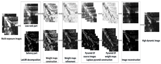
Figure 1.
Framework of the proposed method.
3.1. Generation of Multi-Exposure Images
For practical engineering applications, it is difficult to obtain multi-exposure images without adding additional sensors. Digital TDI brings a new opportunity for high dynamic fusion [35]. The fundamental principle is to improve the sensitivity of the system by multiple exposures to the same target by delay integration. For the global exposure mode, the target is exposed in each frame cycle to obtain one image at a time. N images corresponding to the same ground scene are digitally superimposed to realize N series TDI imaging in the digital domain. Different integral series images can be obtained in the process of digital TDI imaging, and images with a low integral series are equivalent to the low-exposure images, and images with a high integral series are equivalent to the high-exposure images. At the same time, according to the orbit altitude, satellite flight speed and exposure time of the remote imaging sensor, it can be seen that the considerable motion between multi-integral images is far less than one pixel. Therefore, the multi-exposure images produced in this way can be regarded as images of static scenes, which is convenient to the MEF method. We analyze the performance of images with different TDI series. The relations between information entropy and mean gradient and the TDI series are examined as shown in Figure 2. It can be seen that both increase first and then decrease. Thus we can calculate the summation (marked as ) of the information entropy and mean gradient for each integral series. After that, the average value of can be calculated. The relative minimum and maximum integral series can be found for which the value of just exceed the average value. At the same time, the image with the largest value of is involved in fusion. In this way, three images with different series can be selected to participate in the fusion to ensure the quality of the high-dynamic image. However, in practical application, if the memory on-board is sufficient, then more than three images with different TDI series can be chosen to improve the image quality. Without loss of generality, this paper describes images with K integral series selected as low-dynamic images.
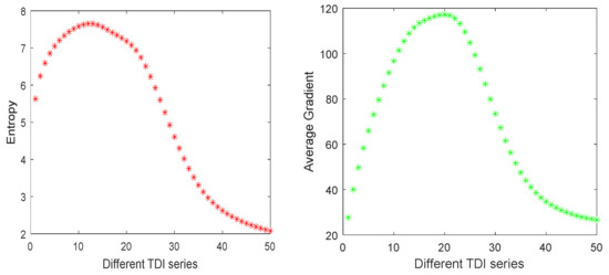
Figure 2.
The correlation between information entropy and mean gradient with TDI series.
3.2. Latent Low-Rank Image Decomposition
To improve the signal-to-noise ratio (SNR) of the fusion image under low illumination, LatLRR is utilized to decompose the source images. LatLRR is more efficient and robust to noise and outliers [36]. An example of LatLRR decomposition using Equation (1) is shown in Figure 3. Figure 3a is the original image. Figure 3b shows the low-rank part of the image, Figure 3c depicts the saliency features and Figure 3d depicts the noise in the 3D display.
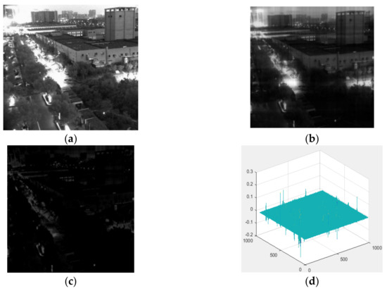
Figure 3.
The LatLRR decomposition. (a) original image; (b) the approximate part; (c) the saliency part; (d) the sparse noise.
The decomposed image sequence is obtained as: and . and are the low-rank and saliency part of the k-th image, respectively. In the following process, they are treated separately and synthesized in the end to remove the effect of noise.
3.3. Weight Map Construction
For the multi-exposure fusion of gray images, weight factors directly affect the fusion effect, and different weights factors are designed for gray images considering the LatLRR decomposition.
3.3.1. Low Rank Part
The low-rank part contains global information, energy information, and brightness and contrast information of the image. First, a contrast factor is constructed according to the fact that the Laplace operator is isotropic. The image is filtered to obtain the high-frequency information by Equation (6). A Gaussian low-pass filter is applied to the absolute value of to obtain the contrast map .
where, is the k-th low-rank image, is the Laplacian operator and represents the convolution operation. is the high-frequency information of the image, and is a symbol of two-dimensional Gaussian filter, the variance of Gaussian filter kernel is 0.5 and the filtering radius is 5. represents the absolute value.
Second, the image exposure is considered. The idea of calculating the exposure factor in [15] is that after normalization of the image, a gray value close to 0.5 is considered to be moderately exposed and is given a larger weight. When deviating from 0.5, the exposure is insufficient or overexposed, and a smaller weight value is given. The method used by [15] misfits the case in which the overall value of an image is too bright or too dark. Under low-light imaging compared to normal light conditions, the overall luminance value is lower in both high and low exposure images. When the whole image intensity is too bright, a darker pixel value should be given a larger weight. By contrast, when it is too dark, a brighter pixel should be given a larger weight. This paper aims at low-illumination imaging, and gray values are lower than normal illumination on the whole. For this reason, the following formulas are designed:
where, 0.8 and 0.2 are empirical parameters that come from a large number of experimental statistics. is the gray value of the k-th low-rank image at . The gray value is normalized to [0,1], and represent the maximum and minimum values of , respectively. represents the mean value of the image. is the standard deviation and is an empirical parameter set to 0.5 in this paper [15,28]. From Equation (10) it can be seen that is a relatively large value when the overall gray value of the image is low, so a large gray value will be given a larger weight by Equation (9) and vice versa.
At last, an initial weight map of the low-rank part is constructed by using the contrast weight and exposure weight together in Equation (11):
According to different images, the fixed proportional factor and cannot guarantee the robustness of the algorithm. Addressing the above issue, an energy function for and is proposed:
The constraints of the upper energy equation are as follows: and, . and are calculated by Equations (5) and (6). k is the serial number of the image. denotes the pixel position. K is the total number of image sequences. The closer the image exposure is to 0.5, the smaller the E value; at the same time, the greater the contrast of adjacent pixels, the smaller the E value. The process of finding the optimal solution involves minimizing the linear energy equation. It can be seen that the weight factors obtained in this way will adapt to different input images to preserve more details.
3.3.2. Saliency Part
The saliency part contains prominent local features and special brightness distributions. The structural and texture factor are combined to construct the fusion factor of the salient part in this paper. The fusion of the saliency part aims at preserving the details of all input images as much as possible. This paper proposes a texture factor of the saliency part designed as Equation (13).
The first term is the norm of the image, and is the average value of the k-th saliency image. When the norm of the image becomes larger, the image has more abundant texture and detail information, and should be given a larger weight value for the corresponding texture. The second term is the Gabor value of the image calculated by Equation (14).
where , and . is expressed in pixels when participating in the calculation. Moreover, represents the multiplication of the corresponding position of the matrix. In general, it is less than one-fifth the size of the input image and greater than or equal to 2. represents the direction of the Gabor filter, and ranges from 0° to 360°. is the phase offset that ranges from −180° to 180°. is used to adjust the elliptic aspect ratio after the Gabor transform. When equals 1, the shape is approximately circular. is the standard deviation of the Gaussian function in the Gabor function. is a gain parameter and is set to 3. We selected the following parameters through extensive experimentation about statistical texture features: , , , , and . The design strategy of parameters selection ensures that the half-peak magnitude supports of the filter responses in the frequency spectrum touch each other in most of the experimental images [37].
3.4. Weight Maps Refinement
The construction of initial weight factors of the low-rank and saliency parts written as and and they have been completed through the above steps. Then, an improved guided filtering is used to suppress artifacts and avoid the block effect due to the lack of spatial consistency in the fusion process.
From Equation (4) we can see that a fixed regularization factor was applied to different local regions in original guided filtering, and the difference in image texture between different regions is not taken into consideration. The adaptive weight factor based on the image gradient is proposed to adjust and an improved guided filtering is proposed to refine weight maps. For and , the calculation process of their regularization factors is not discussed separately, and only the guide image is different. Weight coefficients and of the k-th image were filtered, and guide images of them are the low-rank part and the saliency part of the k-th image obtained by LatLRR decomposition in Section 3.2. In the process of calculating the regularization factor, the low-rank part and the saliency part are uniformly represented as . In this paper, is used to represent the guided filtering operation. is the original weight coefficient, and the is the filtered weight coefficient. For pixel of , the adaptive weight factor is , and the regularization factor is replaced by to improve the robustness of the improved adaptive guided filter. First, the gradient of a guided image is calculated by Equation (15):
where , , and is the gradient image. represents the convolution operation. Values of and are as follows:
The weight factor of pixel in the gradient image is calculated using the following equation:
where and are the variances of region A1 and A2, respectively; and and are the average values of regions A1 and A2, respectively. A1 and A2 are centered on , the size of A1 is 3 × 3, and A2 is the shaded area as shown in Figure 4. and are small numbers to avoid the instability caused by approaching 0, and their values are set to . is set to 0.04, the regularization factor is obtained in this way. Generally, of an edge position is larger than that of a flat area, and the smoothing force of the guided filter is smaller, and vice versa.
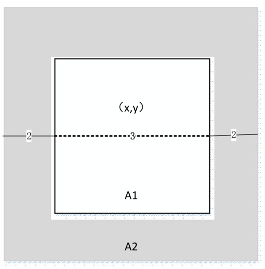
Figure 4.
Schematic drawing of gradient calculation.
Finally, the guided filter is improved by replacing the original regularization term with to prevent insufficient or excessive smoothing in some regions. The refined weight maps of the low-rank and saliency parts by the improved filtering are shown below:
where, weight coefficients and of the k-th image were filtered, and guide images are the low-rank part and the saliency part of the k-th image obtained by LatLRR decomposition in the Section 3.3. and are weight factors after improved guided filtering. And is the size of a local window. Finally, the weights of K images need to be normalized to and , and an example of weight maps refinement is given in Figure 5.
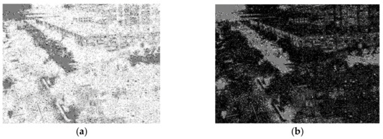
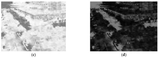
Figure 5.
An example of weight maps refinement. (a) the low-rank weight map; (b) the saliency weight map; (c) the refined low-rank weight map; (d) the refined saliency weight map.
3.5. Multi-Scale Fusion
First, the image sequence of the low-rank part and of the saliency part are fused in Laplacian multi-scale space to obtain the low-rank and saliency parts of multi-exposure fusion, respectively. And the reconstructed low-rank and saliency parts are recorded as and . The construction and refinement of weight maps have been discussed in the above sections. The weight map of a Gaussian pyramid is generated based on and . This process is similar to that of the method in [15]. Second, the HDR image is obtained by the following formula:
The details of our MEF method is as follows:
| Algorithm: MEF Method Proposed by This Paper. |
| Input: K images of different digital TDI levels; |
| Output: High-dynamic fusion image ; |
|
|
|
|
|
|
4. Experimental Results and Analysis
We select 20 sets of static scene images with different TDI series under low illumination to verify the performance of the proposed method. The test sets include representative indoor and outdoor images. Four state-of-the-art algorithms in [15,16,28,29] are chosen to cover a diverse types of MEF methods in terms of methodology and behavior. The method in [16] developed a virtual image based on the gradients of input images. The method in [15] is the classic multi-exposure fusion in multi-scale space, and the construction in multi-scale space used by this paper is based on the method in [15]. The methods in [28,29] are based on patch decomposition, and an image is divided into three conceptually independent components: signal strength, signal structure, and mean intensity. Upon fusing these three components separately, a desired patch is reconstructed and the fusion image can be obtained. And this process is similar to that in our paper. The image is decomposed by LatLRR and then the image is fused by inverse transformation in this paper. Therefore, these four representative methods are chosen for the comparison. Due to space constraints, only the fusion images of reference [15,16,29] are provided here. However, all evaluation indicators of the four methods are calculated and given in the paper. The existing data sets are mostly color images and are taken under normal illumination, while this paper is aimed at gray image fusion under low illumination. The images under the low illumination used by this paper are obtained by a low-illumination camera Gense400BSI in digital TDI imaging mode. The size of the images used by this paper is mostly 1000 × 1000. Experimental data are available and can be download at “https://pan.baidu.com/s/1NTccS607zFEtWJ4VKdn4cQ” and the password is “ntyy”.
The proposed method consists of two types of parameters including the LatLRR decomposition and a guided filter. in LatLRR is set to 0.8. The maximum number of iterations is 50. If images contain excessive noise, the parameter can be appropriately increased. Guided filtering based on the proposed adaptive factor involves only one parameter with the size of 3 × 3. Other parameters involved are described in the paper. All experiments are implemented in MATLAB 2016a on a computer with an Intel Core i7, 3.40-GHz CPU, 16 GB of RAM, and the Microsoft Windows 7 operating system.
4.1. Subjective Analysis
The experimental results of different methods for the target plate image are shown in Figure 6. The overall appearance of all methods is good, and the dynamic range of the image is enhanced from (b)~(e). However we can see that details of the green border are different from Figure 6j–m. Other methods lost details in the bright area, and the target information was lost. The proposed method better preserves the details, and the overall appearance of the fusion image is more appealing. From images (f)~(i), it can be seen that the image noise is high and the uniform wall is distorted by the method in [15,16]. The saturation factor in [15] is no longer suitable for gray images. Compared to the two methods, the patch decomposition approach made some progress in keeping details of the highlighted areas. The uniform whiteboard area is selected to calculate the SNR of the fusion images. The SNRs of the methods in [15,16,29] and our method are 32.4023, 32.6441, 31.1991 and 34.2309, respectively. It can be seen that under low- illumination imaging, the obvious advantage of this paper is denoising by using low-rank decomposition.
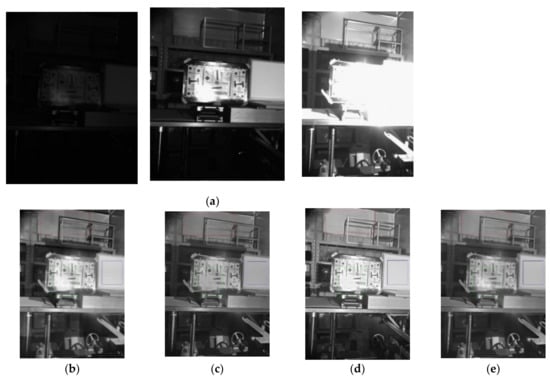
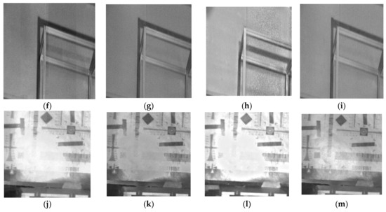
Figure 6.
The comparison of different methods. (a) Source image sequence. (b) The fusion image of [16]. (c) The fusion image of [29]. (d) The fusion image of [15]. (e) The fusion image of our method. (f) Local image of method [16]. (g) Local image of method [29]. (h) Local image of method [15]. (i) Local image of our method. (j) Local image of method [16]. (k) Local image of method [29]. (l) Local image of method [15]. (m) Local image of our method.
Figure 7 shows the fusion images of ‘‘Outdoor Roads’’. The proposed method preserves the information of most of the highlighted areas, and the whole image has better clarity and contrast as shown in Figure 7e. Mertens and the gradient method have better effect than patch decomposition in maintaining load information as shown Figure 7f–i. However, overall, the indication label on the road is visible, and the results by Mertens and the proposed method have more natural appearance with respect to the human visual system. Comparatively, the details and texture of the door are clear by the proposed method in Figure 7i, and the tree texture and numbers in the road are clear as shown in Figure 7m,q. The proposed method effectively preserves details in the brightest and darkest regions. Guided filtering based on an adaptive factor is used to avoid over-smoothing or under-smoothing, effectively reducing the block effect.
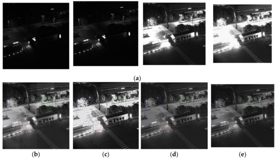
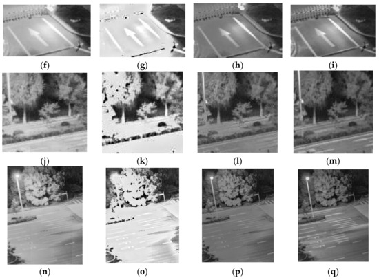
Figure 7.
Comparison of different methods for the outdoor roads. (a) Source image sequence. (b) The fusion image of [16]. (c) The fusion image of [29]. (d) The fusion image of [15]. (e) The fusion image by our method. (f) The local image of by [16]. (g) The local image of [29]. (h) The local image of [15]. (i) The local image by our method. (j) The local image by [16]. (k) The local image by [29]. (l) The local image by [15]. (m) The local image by our method. (n) The local image by [16]. (o) The local image by [29]. (p) The local image by [15]. (q) The local image by our method.
Figure 8 shows the roads and buildings after multi-exposure fusion. The overall contrast of all fusion images is lower. The images are taken at night, and the texture of the ground is clear as shown in Figure 8i. The proposed method and the method in [16] achieved better results for the wall, and the gray distribution of the wall is uniform without super-saturation as shown in Figure 8j,m.
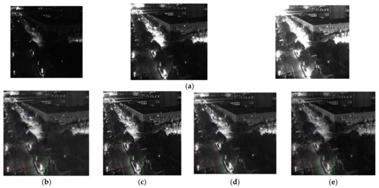
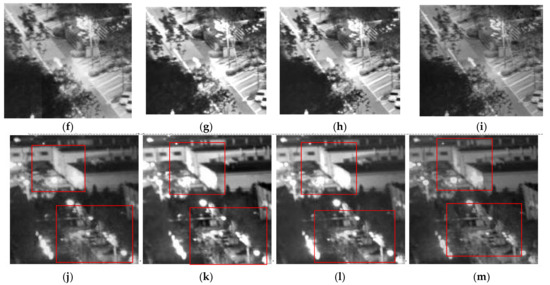
Figure 8.
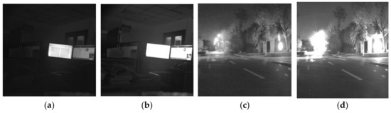
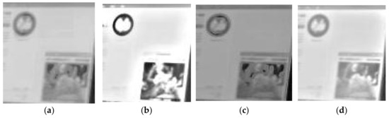
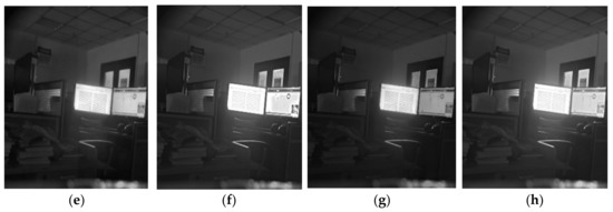
Comparison of different methods on the buildings. (a) Source image sequence. (b) The fusion image of [16]. (c) The fusion image of [29]. (d) The fusion image of [15]. (e) The fusion image of our method. (f) The local image by [16]. (g) The local image by [29]. (h) The local image by [15]. (i) The local image by our method. (j) The local image by [16]. (k) The local image by [29]. (l) The local image by [15]. (m) The local image by our method. The original low dynamic images are shown in Figure 9. Figure 10 shows the MEF fusion of computer screen images taken in the door. Overall, all four methods have restored some desk information and obtained computer screen information, as shown in Figure 10e–h. Moreover, local images are shown in Figure 10a–d. As shown from the local images, we can see that for the icon at the top left corner and the picture at the lower right corner of the computer in the highlighted area, the proposed method maintains better details and contour information, and the grayscale distribution of our method is natural at the same time. However, other images bring gray distortion to different degree.
Figure 11 shows outdoor images with noise. The image with a low TDI series (short exposure) has higher noise under low-light imaging as shown in Figure 9c. The fusion image by this paper has fewer halos around lights and has a relatively clear texture of trees near the lights as show in Figure 11d. The image noise is reduced by our method in uniform sky area as shown in Figure 11h.
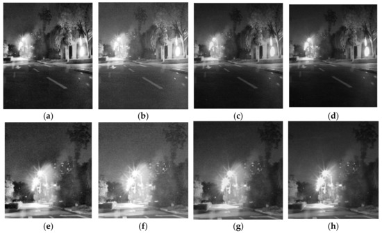
Figure 11.
Comparison of different methods of outdoor images. (a) The fusion image of [16]. (b) The fusion image of [29]. (c) The fusion image of [15]. (d) The fusion image of our method. (e) The local image of [16]. (f) The local image of [29]. (g) The local image of [15]. (h) The local image of our method.
4.2. Objective Analysis
To quantitatively evaluate the performance of the proposed method, three objective indicators including mutual information (MI), edge retentiveness (Q AB/F) and average gradient (AG) are chosen [38]. The MI value can be used to measure how much information from the original image is retained in the fusion image [29,32]. The AG value can sensitively reflect the details of the image, and can be used to evaluate the image blur [31,33]. Q AB/F measures how well the amount of edge information is kept in the fusion images [31]. For all three indicators, the larger the value is, the better the image quality. MI is defined as the sum of mutual information between each source image and the fusion image. The MI value reflects the total quantity of information in the fused image which is obtained from the input source images. For more than two images involved in multi-exposure fusion, Q AB/F is defined as the average of the value calculated by any two images and the fusion image [31]. Four state-of-the-art MEF algorithms in [15,16,28,29] are adopted to fuse 20 groups of gray images with different TDI series under low illumination.
The performance of the four algorithms is shown in Table 1, Table 2 and Table 3, and the largest indicator value is shown in bold. It is clear that the proposed method performs better than the other methods. They are almost the best values in all results. For the indicator MI and Q AB/F, the proposed method shows the best performance in 16 sets of image sequences. Moreover, for the rest of the image sequences, our method ranks in the top two overall. For the indicator AG, the proposed method shows the best performance in 14 sets of image sequences. Even if not the maximum, the indicators are relatively large. The proposed method preserves more detailed information than the other fusion methods and produces fewer artifacts and less noise.

Table 1.
Objective evaluation results of MI.
Table 2.
Objective evaluation results of Q AB/F.
Table 3.
Objective evaluation results of AG.
4.3. Self-Comparison
To further verify advantages of some new ideas proposed by our method, we compared the fusion effect of the following three conditions marked as Con1, Con2 and Con3:
- Con1: using the fixed proportion factor ( = 1 and = 1) and not using the adaptive weight factor by Equation (12);
- Con2: using the original guided filtering and not using the improved guided filtering by Equations (15)–(19);
- Con3: using the weight map construction only by contrast factor and not using Equations (6)–(14).
In each case, we guarantee one single variable. This means there is only one strategy participating in the comparison changes, and the rest remains the same. The results of the above comparison are shown in Table 4, and it represent the average value of 20 sets of data.
Table 4.
The objective evaluation for self-comparison.
In Table 4, a comparison between each row and the last row reflects the improvement on the overall performance under the corresponding conditions. It can be seen from the first row that the energy equation proposed in this paper obtains the adaptive proportional factor ( and ), which mainly affects the information entropy, and can ensure that the HDR image retains as much detail as possible. The second row shows that AG and Q AB/F greatly decrease when the improved guide filter is not used. The improved guided filtering avoids the over-smooth and under-smooth and is helpful in keeping the edge information. We can see from the third row that the weight map designed by our method for gray images under low-illumination imaging can maintain the detail in the process of high-dynamic fusion and has a great influence on all indicators.
To show the visual effect of the proposed ideas on the performance of our method more clearly, one comparative experiment is added. The fusion effect under three different situations is compared as shown in Figure 12. Figure 12a shows that the fixed factor ( = 1 and = 1) cannot adjust the proportion of weight maps in the fusion process adaptively, leading to losses in detail. It can be seen from Figure 12b that in the absence of adaptive guided filtering, the block effect is relatively large, and the ability of edge protection is not sufficient. It is not difficult to find this from Figure 12c without using weight maps proposed in the paper, the image representation ability is reduced, and details of the fusion image in the highlighted and darkened areas are obviously lost.
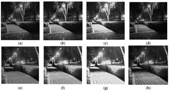
Figure 12.
The result of self -comparison. (a) The result of condtion1. (b) The result of condtion2. (c) The result of condtion3. (d) Our method. (e) The local image of condtion1. (f) The local image of condtion2. (g) The local image of condtion3. (h) The local image of our method.
4.4. Time Complexity Comparison
First, the complexity and efficiency of different algorithms are evaluated by the running time as shown in Table 5. These methods are representative of their fields. The more images involved in the fusion, the longer the processing time. Here, we consider two images involved in the calculation. The size of the images used by this paper is mostly 1000 × 1000. The average time is taken as the contrast result. Different iteration numbers of LatLRR used by our method are adopted. For an image with the size of 1000 × 1000, the super-pixel segmentation approach method used by reference [29] specifies the number of super-pixels as 200, and the fixed-sized patches are rectangles of 50 × 50 used by reference [28].
Table 5.
Running time of different methods (seconds).
The methods in [15,16] are relatively efficient in running time. The weight calculation of both methods is relatively simple. An intermediate image is constructed in the gradient domain by method [16], which takes more time than that in [15]. The execution efficiencies of method [28] and the proposed method applying 20 iterations are not much different. Our method is time-consuming in the stage of low rank decomposition. The patch and structure decomposition technique is used in method [28,29], and it is time-consuming to compare and calculate parameters between blocks. Compared with the methods in [28,29] and our method, the method in [23] is more efficient. In addition, the time-consuming nature of this method depends mainly on the number of pyramid layers. The method in [33] divided the multi-exposure image into image detail layer and a contour layer by image decomposition. Moreover, for the image detail layer, a CNN network is used to achieve detail-layer fusion. This is relatively time-consuming. The CNN and sparse representation algorithm require too much time due to their own operating schemes.
Second, the running time for applying 10, 20 and 30 iterations of our method is counted as shown in Table 6. With an increase in the number of iterations, the running time of our method increases significantly. The main time-consuming item in this paper is the low-rank decomposition. The effect of the iteration number on the fusion performance is also analyzed, as shown in Table 6. The result in Table 6 is the average value of 20 sets of data. It is clear that with the increase of iteration numbers, the performance improves gradually, but the difference between 20 iterations and 30 iterations is not obvious. The number of iterations can be selected according to the practice requirement. At the same time, without increasing the amount of computation, the method of selecting the optimal iteration number used by our paper is given here. LatLRR is utilized to decompose the source image into global and local structure. We calculate the information entropy of the global structure image produced by different iterations. When the number of iterations increases, the information entropy changes slightly, and the iteration can be stopped, or the maximum number of iterations is reached. When ensuring that the indicator can meet the actual requirement, a relatively small number of iterations can be chosen.
Table 6.
Objective evaluation of indicators for the proposed method of different iterations.
In summary, our method is not the fastest, and the running time increases as the iteration time increases, but this method is still efficient and compromises between the running time and quality.
5. Conclusions and Future Work
In this paper, a multi-exposure fusion of gray images under low illumination based on low-rank decomposition was presented. The latent low-rank representation was used on low-dynamic images to generate low-rank parts and saliency parts to reduce noise after fusion. The idea of this paper was to decompose image sequences separately in multi-scale space. Thus, two different weight maps were constructed according to features of gray images. To remove the artifacts, an improved guided filtering method based on an adaptive regularization factor was proposed to refine the weight maps. At the same time, the adaptive ratio of weight factors was calculated based on an energy equation to enhance the robustness of the method. Then, the decomposed low-rank images and saliency images were fused in Laplacian space using Gaussian pyramid weight factors to obtain a fused low-rank image and a fused saliency image. Finally, the high-dynamic image was reconstructed by adding the low-rank image and the saliency image.
Although the proposed method can produce high-quality in high dynamic images under low-illumination imaging, it is not suitable for real-time application. Remote sensing images have a large amount of data; therefore, the algorithm should be optimized to improve the efficiency for practical engineering applications.
Author Contributions
T.N. provided the idea. T.N., H.L. and L.H. designed the experiments. X.L., H.Y., X.S., B.H. and Y.Z. analyzed the experiments. T.N. wrote the paper. All authors have read and agreed to the published version of the manuscript.
Funding
This research was funded by the National Natural Science Foundation of China grant number No.62005280.
Institutional Review Board Statement
Not applicable.
Informed Consent Statement
Not applicable.
Data Availability Statement
The data presented in this study are available in the article.
Acknowledgments
The authors wish to thank the associate editor Summer Ang and the anonymous reviewers for their valuable suggestions.
Conflicts of Interest
The authors declare no conflict of interest.
References
- Lin, J.; Li, M.; Yu, D.; Tang, C. Realization of imaging system of low light level night vision based on EMCCD. In Proceedings of the 2nd International Conference on Measurement, Information and Control, Harbin, China, 16–18 August 2013; pp. 345–349. [Google Scholar]
- Wang, Y.; Liu, H.; Fu, Z. Low-light image enhancement via the absorption light scattering model. IEEE Trans. Image Process 2019, 28, 5679–5690. [Google Scholar] [CrossRef] [PubMed]
- Guo, X.; Li, Y.; Ling, H. LIME: Low-light image enhancement via illumination map estimation. IEEE Trans. Image Process 2017, 26, 982–993. [Google Scholar] [CrossRef] [PubMed]
- Ying, Z.; Li, G.; Ren, Y.; Wang, R.; Wang, W. A new low-light image enhancement algorithm using camera response model. In Proceedings of the IEEE International Conference on Computer Vision Workshops (ICCVW), Venice, Italy, 22–29 October 2017; pp. 3015–3022. [Google Scholar]
- Yang, Y.; Cao, W.; Wu, S.; Li, Z. Multi-Scale Fusion of Two Large-Exposure-Ratio Images. IEEE Signal Process. Lett. 2018, 25, 1885–1889. [Google Scholar] [CrossRef]
- Debevec, P.E.; Jitendra, M. Recovering high dynamic range maps from photographs. In Proceedings of the 24th Annual Conference on Computer Graphics and Interactive Techniques; ACM: New York, NY, USA, 1997. [Google Scholar]
- Reinhard, E.; Stark, M.; Shirley, P.; Ferwerda, J. Photographic tone reproduction for digital images. ACM Trans. Graph. 2002, 21, 267–276. [Google Scholar] [CrossRef]
- Fattal, R.; Lischinski, D.; Werman, M. Gradient domain high dynamic range compression. ACM Trans. Graph. 2002, 21, 249–256. [Google Scholar] [CrossRef]
- Li, T.; Xie, K.; Li, T.; Sun, X.; Yang, Z. Multi-exposure image fusion based on improved pyramid algorithm. In Proceedings of the 2020 IEEE 4th Information Technology, Networking, Electronic and Automation Control Conference (ITNEC), Chongqing, China, 12–14 June 2020; pp. 2028–2031. [Google Scholar] [CrossRef]
- Shen, J.; Zhao, Y.; Yan, S.; Li, X. Exposure fusion using boosting Laplacian pyramid. IEEE Trans. Cybern. 2014, 44, 1579–1590. [Google Scholar] [CrossRef]
- Kou, F.; Li, Z.; Wen, C.; Chen, W. Edge-preserving smoothing pyramid based multi-scale exposure fusion. J. Vis. Commun. Image Represent. 2018, 53, 235–244. [Google Scholar] [CrossRef]
- Prabhakar, K.R.; Srikar, V.S.; Babu, R.V. Deepfuse: A deep un-supervised approach for exposure fusion with extreme exposure image pairs. In Proceedings of the IEEE International Conference on Computer Vision Workshops (ICCVW), Venice, Italy, 22–29 October 2017; pp. 4724–4732. [Google Scholar]
- Wang, Q.T.; Chen, W.H.; Wu, X.M.; Li, Z.G. Detail preserving multi-scale exposure fusion. In Proceedings of the IEEE International Conference on Image Processing (ICIP), Athens, Greece, 7–10 October 2018; pp. 1713–1717. [Google Scholar]
- Que, Y.; Yang, Y.; Lee, H.J. Exposure measurement and fusion via adaptive multi-scale edge-preserving smoothing. IEEE Trans. Instrum. Meas. 2019, 68, 4663–4674. [Google Scholar] [CrossRef]
- Mertens, T.; Kautz, J.; van Reeth, F. Exposure fusion: A simple and practical alternative to high dynamic range photography. Comput. Graph. Forum 2009, 28, 161–171. [Google Scholar] [CrossRef]
- Paul, S.; Sevcenco, I.S.; Agathoklis, P. Multi-exposure and multi-focus image fusion in gradient domain. J. Circuits Syst. Comput. 2016, 25, 1650123.1–1650123.18. [Google Scholar] [CrossRef]
- Li, Z.; Wei, Z.; Wen, C.; Zheng, J. Detail-enhanced multi-scale exposure fusion. IEEE Trans. Image Process. 2017, 26, 1234–1252. [Google Scholar] [CrossRef] [PubMed]
- He, K.; Sun, J.; Tang, X. Guided image filtering. IEEE Trans. Pattern Anal. Mach. Intell. 2012, 35, 13971409. [Google Scholar]
- Liu, S.; Zhang, Y. Detail-preserving underexposed image enhancement via optimal weighted multi-exposure fusion. IEEE Trans. Consum. Electron. 2019, 65, 303–311. [Google Scholar] [CrossRef]
- Zhang, W.; Cham, W.K. Gradient-directed multi-exposure composition. IEEE Trans. Image Process. 2011, 21, 2318–2323. [Google Scholar] [CrossRef]
- Lee, S.H.; Park, J.S.; Cho, N.I. A multi-exposure image fusion based on the adaptive weights reflecting the relative pixel intensity and global gradient. In Proceedings of the 2018 25th IEEE International Conference on Image Processing (ICIP), Athens, Greece, 7–10 October 2018. [Google Scholar]
- Fan, H.; Zhou, D.M.; Nie, R.C. A color multi-exposure image fusion approach using structural patch decomposition. IEEE Access 2018, 6, 42877–42885. [Google Scholar]
- Chen, G.; Li, L.; Jin, W.Q.; Qiu, S.; Guo, H. Weighted sparse representation and gradient domain guided filter pyramid image fusion based on low-light-level dual-channel camera. IEEE Photon. J. 2019, 11, 5. [Google Scholar] [CrossRef]
- Srivastava, R.; Singh, R.; Khare, A. Image fusion based on nonsubsampled contourlet transform. In Proceedings of the 2012 International Conference on Informatics, Electronics & Vision (ICIEV), Dhaka, Bangladesh, 18–19 May 2012; pp. 263–266. [Google Scholar]
- Kim, J.; Choi, H.; Jeong, J. Multi-exposure image fusion based on patch using global and local characteristics. In Proceedings of the 2018 41st International Conference on Telecommunications and Signal Processing (TSP), Athens, Greece, 4–6 July 2018; pp. 1–5. [Google Scholar]
- Li, Y.; Sun, Y.; Zheng, M.; Huang, X.; Qi, G.; Hu, H.; Zhu, Z. A novel multi-exposure image fusion method based on adaptive patch structure. Entropy 2018, 20, 935. [Google Scholar] [CrossRef]
- Ma, K.; Yeganeh, H.; Zeng, K.; Wang, Z. High dynamic range image compression by optimizing tone mapped image quality index. IEEE Trans. Image Process. 2015, 24, 3086–3097. [Google Scholar]
- Ma, K.; Li, H.; Yong, H.; Wang, Z.; Meng, D.; Zhang, L. Robust multi-exposure image fusion: A structural patch decomposition approach. IEEE Trans. Image Process. 2017, 26, 25192532. [Google Scholar] [CrossRef]
- Wang, S.P.; Zhao, Y. A novel patch-based multi-exposure image fusion using super-pixel segmentation. IEEE Access 2020, 8, 39034–39045. [Google Scholar] [CrossRef]
- Qi, G.; Chang, L.; Luo, Y.; Chen, Y.; Zhu, Z.; Wang, S. A Precise Multi-Exposure Image Fusion Method Based on Low-level Features. Sensors 2020, 20, 1597. [Google Scholar] [CrossRef] [PubMed]
- Kalantari, N.K.; Ramamoorthi, R. Deep high dynamic range imaging of dynamic scenes. ACM Trans. Graph. 2017, 36, 1–12. [Google Scholar] [CrossRef]
- Prabhakar, K.R.; Arora, R.; Swaminathan, A. A fast, scalable, and reliable deghosting method for extreme exposure fusion. In Proceedings of the IEEE International Conference on Computational Photography (ICCP), Tokyo, Japan, 15–17 May 2019. [Google Scholar]
- Chen, G.; Li, L.; Jin, W. High-dynamic range, night vision, image-fusion algorithm based on a decomposition convolution neural network. IEEE Access 2019, 7, 169762–169772. [Google Scholar] [CrossRef]
- Liu, G.; Yan, S. Latent Low-Rank Representation for subspace segmentation and feature extraction. In Proceedings of the 2011 International Conference on Computer Vision, Barcelona, Spain, 6–13 November 2011; pp. 1615–1622. [Google Scholar]
- Tao, S.; Zhang, X.; Xu, W.; Qu, H. Realize the image motion self-registration based on TDI in digital domain. IEEE Sens. J. 2019, 19, 11666–11674. [Google Scholar] [CrossRef]
- Han, X.Y.; Lv, T.; Song, X.Y.; Nie, T.; Liang, H.D.; He, B.; Kuijper, A. An Adaptive Two-Scale Image Fusion of Visible and Infrared Images. IEEE Access 2019, 7, 56341–56362. [Google Scholar] [CrossRef]
- Manjunath, B.S.; Ma, W.Y. Texture features for browsing and retrieval of image data. IEEE Trans. Pattern Anal. 1996, 18, 837–842. [Google Scholar] [CrossRef]
- Yazdi, M.; Ghasrodashti, E.K. Image fusion based on non-subsampled contourlet transform and phase congruency. In Proceedings of the 19th IEEE International Confernce on Systems, Signals and Image Processing (IWSSIP), Vienna, Austria, 11–13 April 2012; pp. 616–620. [Google Scholar]
Publisher’s Note: MDPI stays neutral with regard to jurisdictional claims in published maps and institutional affiliations. |
© 2021 by the authors. Licensee MDPI, Basel, Switzerland. This article is an open access article distributed under the terms and conditions of the Creative Commons Attribution (CC BY) license (http://creativecommons.org/licenses/by/4.0/).