Optimizing Matching Area for Underwater Gravity-Aided Inertial Navigation Based on the Convolution Slop Parameter-Support Vector Machine Combined Method

Abstract

This paper focuses on the selection of matching areas in the gravity-aided inertial navigation system. Firstly, the Sobel operator was used in convolution of the gravity anomaly map to obtain the feature map. The convolution slope parameters were constructed by combining the feature map and the gravity anomaly map. The characteristic parameters, such as the difference between convolution rows and columns, convolution variance of the feature map, the pooling difference, and range of the gravity anomaly map, were combined. Based on the support vector machine algorithm, the convolution slope parameter-support vector machine combined method is proposed. Second, we selected the appropriate training sample set and set parameters to verify. The results show that compared with the pre-calibration results, the classification accuracy of the test set is more than 92%, which proves that the convolution slope parameter-support vector machine combined method can effectively distinguish between the suitable and the unsuitable area. Thirdly, we applied this method to another region. The navigation experiment was performed in the split-matching area. The average positioning error was better than 100 m, and the correct rate was more than 90%. The results show that sailing in the selected area can accurately match the trajectory and reduce the positioning error.

1. Introduction

In recent years, countries have paid more and more attention to the exploration and utilization of marine resources. The navigation and positioning function of underwater vehicles has gradually become one of the principal directions in scientific research. Because the inertial navigation system (INS) is prone to accumulate errors over time, underwater vehicles need to use other physical information combined with INS for positioning navigation. The gravity-aided inertial navigation system (GAINS) can match the real-time gravity information with the pre-stored marine gravity anomaly map to obtain the accurate position of the underwater vehicle and correct the accumulated error of the INS [1,2,3,4,5,6,7]. The GAINS does not radiate energy or accept electromagnetic signals when obtaining gravity information. It has excellent concealment and is a passive, high-precision underwater navigation system.

The matching effect of GAINS is closely related to the distribution of the gravity field. The matching effect of the area with prominent gravity field characteristics is generally better. When the vehicles pass through the area where the gravity field changes violently, it is easy to find the corresponding trajectory. However, there is no accurate correspondence between the gravity field distribution and the suitability, so it is of great significance to further study the gravity field’s suitability to improve the navigation system’s accuracy.

At present, there is a great deal research on matching area selection. In 2015, Jianqiao Tang and others used the multi-feature fusion method based on full-tensor gravity gradient to select the suitable area. The local standard deviation, local energy, local entropy, roughness, slope, and correlation coefficient parameters were mainly used. The threshold of local standard deviation and local entropy was obtained by the experimental method, which was used as the selection criterion of the suitable area [8]. In 2016, based on the theory of fractal geometry, Bo Wang et al. proposed the isotropic coefficient by analyzing the spectral characteristics of the three-dimensional surface gravity anomaly sequence. Using the analytic hierarchy process to combine the traditional gravity parameters and isotropic coefficients to select the suitable area, the results show that this method has better directionality [9]. In 2017, Hubiao Wang and others analyzed the traditional parameters of the gravity anomaly map, constructed a type of gravity anomaly characteristic parameters, analyzed the influence of gravity changes on the accuracy of GAINS, and determined the positioning accuracy of gravity matching in different regions. Experimental results show that the parameters can better characterize ocean gravity anomaly [10]. In 2019, Fanming Liu and others used the projection pursuit method for suitability analysis, used the image texture feature analysis method to extract the navigability features of the local gravity map, and used the projection pursuit model to comprehensively evaluate the navigability of the local gravity map [11]. In 2019, Bo Wang et al. proposed a vector difference parameter of gravity anomaly, using the entropy weight method to combine the gravity field’s standard deviation, roughness, and vector difference parameters to obtain comprehensive characteristic parameters to select the suitable area. The simulation results show that the suitable area selected by this method is more concentrated and continuous [12]. In 2021, Chenglong Wang and others proposed a suitable area-selection algorithm based on the co-occurrence matrix. The algorithm first establishes the gravity anomaly co-occurrence matrix and calculates the characteristic parameters reflecting the spatial relationship of the gravity field through the gray-scale co-occurrence matrix. The four spatial relationship feature parameters are weighted and summed to establish a comprehensive spatial feature parameter. The suitable area is selected by the criterion of maximizing the variance between classes [13]. In 2021, Chenglong Wang and others also proposed an algorithm based on Delaunay triangulation for underwater GAINS suitable area selection. The algorithm builds a three-dimensional model, extracts spatial feature parameters for gravity field analysis, and finally uses cluster analysis to select the suitable area [14].

Unlike the above processing methods, we used the Sobel operator to convolution the gravity anomaly map and construct the convolution slope parameters. The support vector machine algorithm was used to combine the difference between convolution rows and columns, the variance of the feature map, the pooling difference, and the range of the gravity anomaly map. Then, the classification model was obtained by calculating the data of the training-set area. This classification model was used to divide the test-set area and compared it with the pre-calibration results. Finally, the classification model was used to divide matching areas in another region. The simulation experiment was carried out in the suitable area to further verify the selected area’s suitability.

2. Materials and Methods

2.1. Image Convolution

In this study, the Sobel operator was used for convolution to highlight the high-frequency change part of the gravity anomaly map to effectively distinguish the areas where the gravity anomaly changes drastically. When sailing in east-west direction, the vertical edge-detection operator is used to divide the suitable area; the horizontal edge-detection operator is used when sailing in north-south direction; the 45° edge-detection operator is used for northwest direction, and the 135° edge-detection operator is used for northeast direction. The Sobel operators are as shown in Figure 1 [15,16]. The calculation of each pixel in the feature map is shown in Formula (1). The pixels that cannot be calculated by the Sobel operator in the edge part of the feature map are filled with 0.

$$f(x,y)=\left|{\displaystyle \sum _{u=-1}^1{\displaystyle \sum _{v=-1}^{1}g(x+u,y+v)}\cdot h(2+u,2+v)}\right|$$

(1)

where $f(x,y)$ is the value of coordinate $(x,y)$ in the feature map, $g(x,y)$ is the value of coordinate $(x,y)$ in the gravity anomaly map, and $h(2+u,2+v)$ is the value of coordinate $(2+u,2+v)$ in the Sobel Operator. The variables $u$ and $v$ are added to determine the coordinates of the gravity anomaly map and the Sobel Operator.

2.2. Convolution Slope Parameter

We thus combined the feature map and the gravity anomaly map to construct the convolution slope parameter. Unlike the traditional slope-calculation method, the convolution slope first calculates the single-line slope and then averages it. It considers the overall situation of the gravity anomaly distribution in the target area and can incorporate heading factors. The size of the target area is $M\times N$, and the calculation steps of the slope parameter of the east-west direction are as follows. Similarly, the parameter for other directions can be obtained.

In the first step, the vertical edge-detection Sobel operator is selected for convolution operation, and the points with a value less than 0.1 in the feature map are set to 0. According to the convolution calculation formula, when the result is less than 0.1, the variation amplitude of the left and right sides of the current pixel is tiny. This point can be considered the possible extreme point of the gravity anomaly map along the y-axis direction.

In the second step, we traverse the feature map by row. Each row of data except the beginning and end of the row may have multiple 0 points corresponding to the extreme points of the gravity anomaly in this row; if there is no maximum or minimum point in this row, only the value at the head and tail of this row is 0. We thus record the coordinates of each 0 point in the row and calculate the single-row slope value according to the Formula (2).

$$S_x={\displaystyle \sum _k\frac{\left|g(x,y_{k+1})-g(x,y_k)\right|}{\left|y_{k+1}-y_k\right|}}$$

(2)

where $x$ is the x-axis coordinate of the current row, $y_k$ is the y-axis coordinate of the kth 0 points of the row, and $g(x,y)$ is the gravity anomaly value.

In the third step, the average of all single-row slopes in the target area is used as the convolution slope parameter of the area. The formula is as follows:

$$slop=\frac{{\displaystyle \sum _{x=2}^{M-1}{S}_x}}{M-2}$$

(3)

The denominator is $M-2$ because the edge part of the image is filled with 0 during convolution operation, so the single-row slope values of the first and last rows are not calculated. When calculating the north-south direction convolution slope parameters, the horizontal edge-detection operator is selected, and step two is changed to traverse by column to calculate the single column slope of each column. When calculating the convolution slope parameter of diagonal direction, the diagonal direction edge-detection operator is used to calculate the single-line slope of each diagonal within the track coverage.

2.3. Other Characteristic Parameters

In this paper, when selecting the characteristic parameters, the trajectory mismatch problem was specially analyzed. Suppose the gravity anomaly sequence of the pre-matched track and the actual track are relatively similar. In that case, it cannot effectively distinguish between the two, resulting in track mismatch and thus producing a significant positioning error. Therefore, the difference between convolution rows and columns parameters is proposed. Subsequently, using the convolution variance parameter, the feature map can reflect the change of gravity anomaly in the area. On this basis, the variance of the feature map can reflect the complexity of the fluctuation of gravity anomaly. Finally, considering that the influence of measurement error can be relatively reduced when the span of gravity anomaly value sequence is large, the range and pooling difference parameters were used [17,18]. The pooling difference can reflect the variation amplitude of the gravity anomaly sequence collected when sailing in different directions.

2.3.1. Difference between Convolution Rows and Columns Parameter

Convolution values reflect the variation range of gravity anomaly along with specific directions. The difference between rows and columns of feature maps can more effectively reflect the difference of gravity anomaly sequences between adjacent trajectories. Headings in the east-west direction calculate the difference between the rows, headings in the north-south direction calculate the difference between the columns, and the difference between the oblique lines in the shaded range shown in Figure 2 is calculated when the northeast and northwest directions are sailed. The formula is as follows:

$$D=\left\{\begin{array}{cc}{\displaystyle \sum _{x=1}^{M-2}{\displaystyle \sum _{y=2}^{N-1}\left(f(x,y)-f(x+1,y)\right)}}& \mathrm{East}-\mathrm{West} \mathrm{direction}\\ {\displaystyle \sum _{y=2}^{N-2}{\displaystyle \sum _{x=2}^{M-1}\left(f(x,y)-f(x,y+1)\right)}}& \mathrm{North}-\mathrm{South} \mathrm{direction}\\ {\displaystyle \sum _{x=1}^M{\displaystyle \sum _{y=\max (1,x-M/2)}^{\min (x+N/2,N)}\left(f(x,y)-f(x+1,y+1)\right)}}& \mathrm{Northeast} \mathrm{direction}\\ {\displaystyle \sum _{x=1}^M{\displaystyle \sum _{y=\max (1,N/2-x)}^{\min (3M/2-x,N)}\left(f(x,y)-f(x+1,y-1)\right)}}& \mathrm{Northwest} \mathrm{direction}\end{array}\right.$$

(4)

2.3.2. Convolution Variance

The feature map reflects the change rate of each point in the gravity anomaly map in a specific direction. The more significant the variance of the convolution map is, the more complex the change of the gravity anomaly value in this direction is, and the apparent gravity anomaly sequence feature makes positioning more accurate. The calculation formula is as follows [19]:

$$C=\frac{{\displaystyle \sum _{x=2}^{M-1}{\displaystyle \sum _{y=2}^{N-1}{(f(x,y)-\mu )}^2}}}{(M-2)(N-2)}$$

(5)

where $M\times N$ is the size of the feature map, with $\mu$ indicating the mean value of the feature map. The edge of the feature map is filled with 0, so the range of effective pixels is $\left\{(x,y)|2\le x\le M-1,2\le y\le N-1\right\}$.

2.3.3. Pooling Difference

The essence of the pooling method is to downsample the image data. It is generally believed that the average pooling can better retain the global feature of the data and highlight the background information. When matching in the target area, the length of the navigation trajectory should be more than half of the edge length of the selected area to reflect the suitability of the area accurately. Therefore, in this paper, the edge length of the target area is divided into four equal parts and then subdivided into 16 non-overlapping parts. In this case, each navigation trajectory should span at least three parts. The average of the gravity anomaly of each part is taken as the element value at the corresponding position of the pooling matrix:

$$\left[\begin{array}{cccc}{p}_{11}& p_{12}& p_{13}& p_{14}\\ p_{21}& p_{22}& p_{23}& p_{24}\\ p_{31}& p_{32}& p_{33}& p_{34}\\ p_{41}& p_{42}& p_{43}& p_{44}\end{array}\right]$$

(6)

where $p_{ij}=\frac{{\displaystyle \sum _{x=(i-1)\times L/4}^{i\times L/4}{\displaystyle \sum _{y=(j-1)\times L/4}^{j\times L/4}g(x,y)}}}{{(L/4)}^2}$. The pooling matrix is further processed according to the different navigation directions to obtain the characteristic parameters of the pooling difference. The calculation method of pooling difference corresponding to each direction is as follows:

$$\begin{gathered} P=\left\{\begin{array}{cc}|p_{14}-p_{12}|+|p_{13}-p_{11}|+|p_{24}-p_{22}|+|p_{23}-p_{21}|+ \\ |p_{34}-p_{32}|+|p_{33}-p_{31}|+|p_{44}-p_{42}|+|p_{43}-p_{41}|\hfill & \mathrm{East}-\mathrm{West} \mathrm{direction}\\ |p_{11}-p_{31}|+|p_{21}-p_{41}|+|p_{12}-p_{32}|+|p_{22}-p_{42}|+ \\ |p_{13}-p_{33}|+|p_{23}-p_{43}|+|p_{14}-p_{34}|+|p_{24}-p_{44}|\hfill & \mathrm{North}-\mathrm{South} \mathrm{direction}\\ |p_{13}-p_{31}|+|p_{14}-p_{32}|+|p_{23}-p_{41}|+|p_{24}-p_{42}|\hfill & \mathrm{Northeast} \mathrm{direction}\\ |p_{11}-p_{33}|+|p_{12}-p_{34}|+|p_{21}-p_{43}|+|p_{22}-p_{44}|\hfill & \mathrm{Northwest} \mathrm{direction}\end{array}\right. \end{gathered}$$

(7)

2.3.4. Range

The range can reflect the overall gravity anomaly amplitude in the selected area. Theoretically, when sailing in a region with a large range, the collected gravity anomaly sequence will change significantly, which reduces the influence of measurement error and improving the matching accuracy. The calculation formula is as follows [20]:

$$R=g{(i,j)}_{\max }-g{(i,j)}_{\min }$$

(8)

2.4. Principle of Support Vector Machine Algorithm

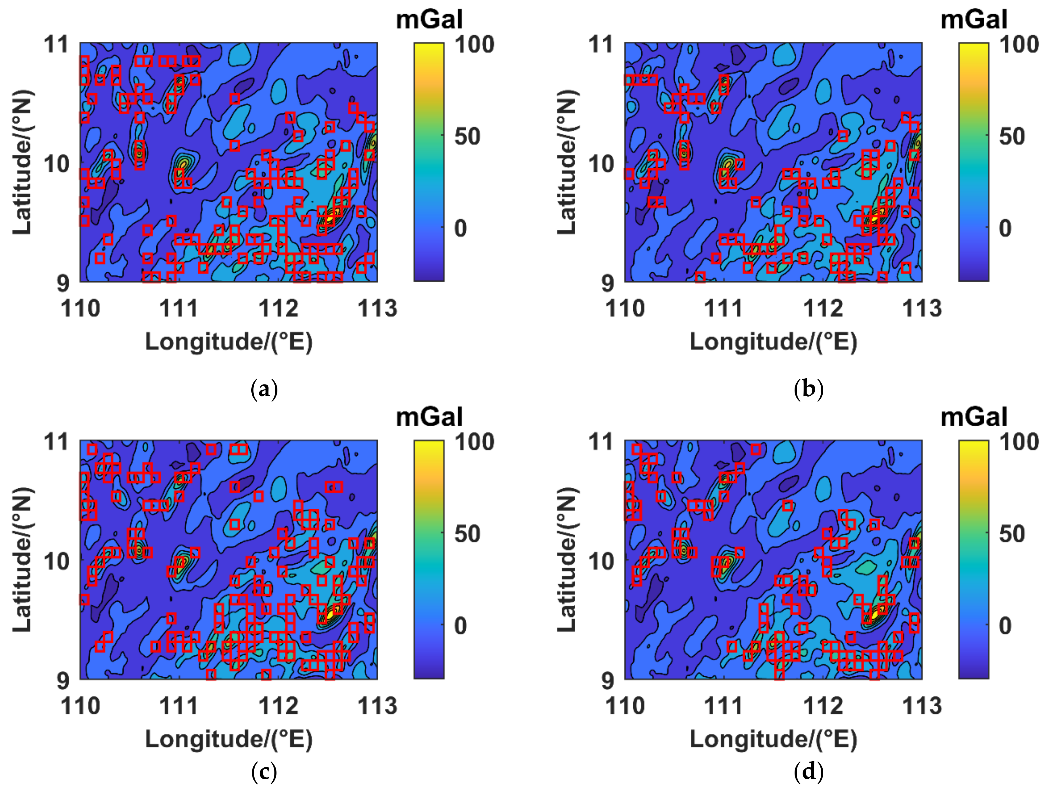
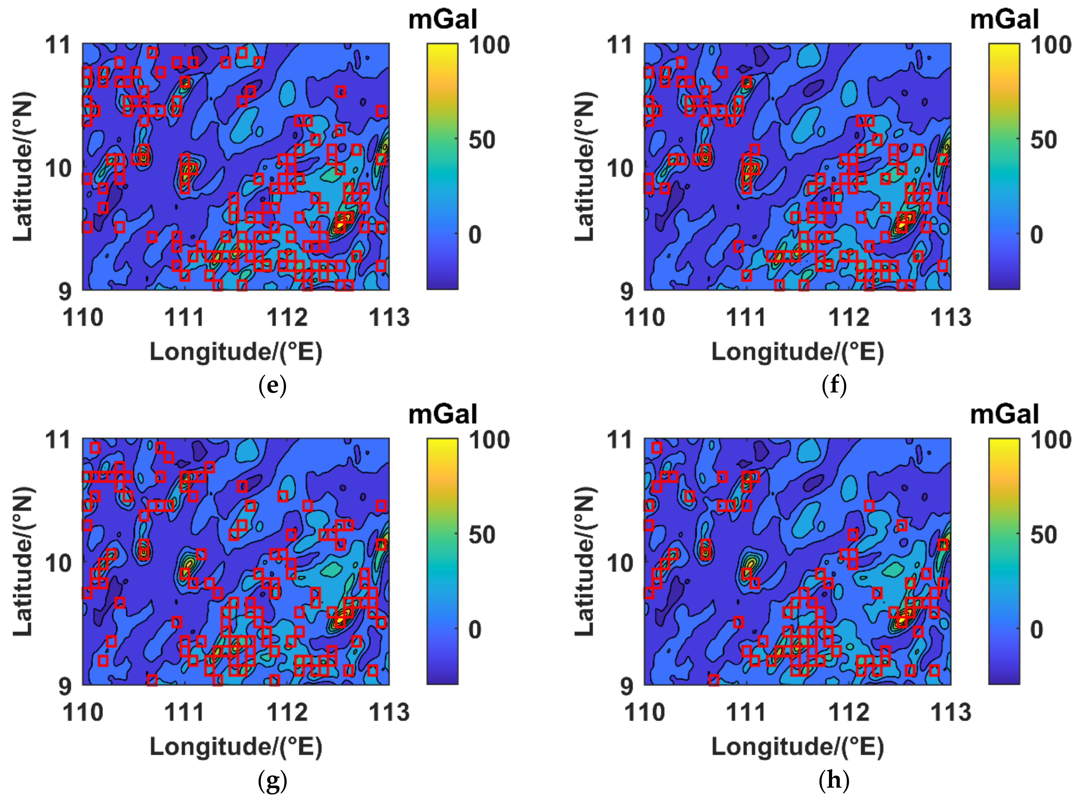
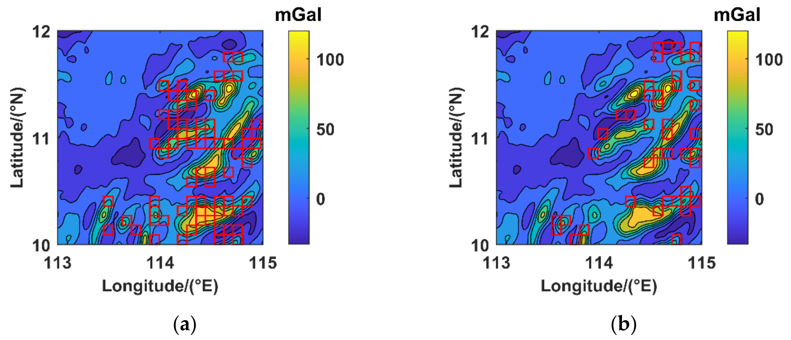
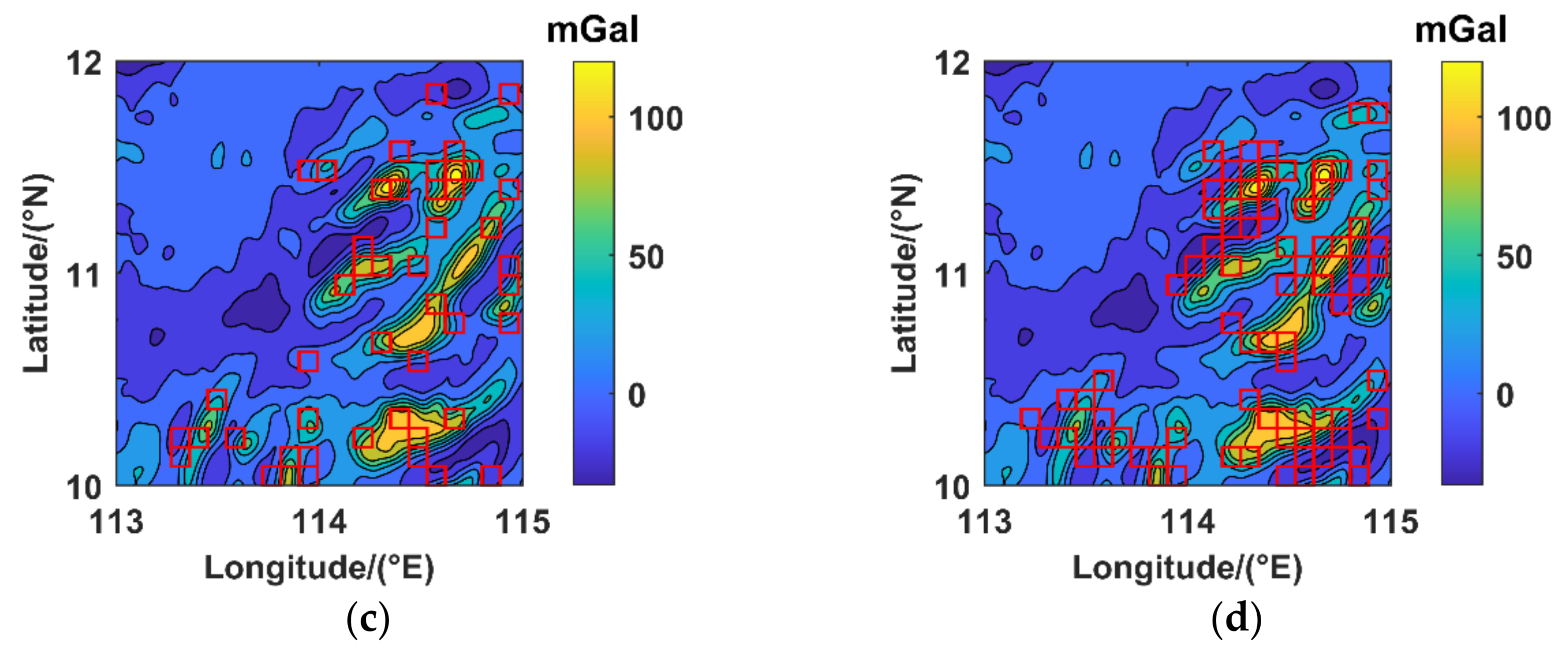
There are significant differences in the value range, unit, or dimension of different characteristic parameters, which will have adverse effects in classification. To eliminate this factor, we adopted the commonly used z-score standardization method to standardize the sample data. The formula is as follows [21]:

$$x_i^{\ast }=\frac{x_i-\mu }{\sigma }$$

(9)

where $\mu$ and $\sigma$ represent the mean and standard deviation of the characteristic parameters $x_i$.

Support vector machine (SVM) is a machine learning method proposed by Vapnik et al. in the 1990s, used to solve classification and regression problems [22,23,24]. It is a supervised learning algorithm that classifies the target samples according to the distribution information of the current samples. The idea of the SVM algorithm is to establish a hyperplane between two types of samples, to maximize the blank area on both sides of the hyperplane while ensuring the classification accuracy to find the optimal solution of the linear classification problem, and finally to obtain the classification discriminant function as follows:

$$f(x)=\mathrm{sgn}\left[\left({\displaystyle \sum _{i=1}{a}_i{y}_{i}K\left(x,x_i\right)}\right)+b\right]$$

(10)

where $x_i$ represents the sample characteristic parameter vector; $y_i$ represents the sample category. The hyperplane equation should be transformed into a constrained optimization problem, and the Lagrange multiplier $\alpha$ and offset vector $b$ should be solved by the sequential minimum optimization algorithm. When the characteristic parameters are linearly inseparable, introducing kernel function to increase the dimension of the feature vector may make the feature vector better divided in high-dimensional space, so the selection of kernel function has a significant influence on the classification effect. Usually, in the absence of prior information, using the Gaussian radial basis function kernel is better, the specific form is: $K\left(x,x_i\right)=\exp \left(-\gamma {‖x-x_i‖}^2\right)$.

In this paper, the accuracy and single-class recall rate are used to further evaluate the effectiveness of the classification model. The accuracy, C, and single-class recall rate, R, are defined as follows [25]:

$$C=\frac{{\displaystyle \sum _{i=1}^{2}N(x_p\in {\omega }_i\cap x_r\in {\omega }_i)}}{N(x)}$$

(11)

$$R_i=\frac{N(x_p\in {\omega }_i\cap x_r\in {\omega }_i)}{N(x_r\in {\omega }_i)},i=1,2$$

(12)

where ${\omega }_1$ and ${\omega }_2$ represent the suitable and unsuitable areas, $x_p$ represents the classification results of the classification model for sample $x$, $x_r$ represents the category of sample $x$ in the pre-calibration results, and $N\left(x_p\in {\omega }_i\cap x_r\in {\omega }_i\right)$ represents the number of samples in which the classification model and the pre-calibration results are the same as ${\omega }_i$.

3. Results

3.1. Verification

We used gravity anomaly data from the University of California San Diego website (http://topex.ucsd.edu/, accessed on 15 August 2021) with the resolution of $1’\times 1’$. Some regions in the South China Sea were selected for research. The longitude and latitude ranges are 110°E−113°E and 9°N−11°N. Then, MATLAB software was used for linear interpolation of the region. The spatial resolution of the interpolation image is approximately 100 m × 100 m, as shown in Figure 3. The maximum value of gravity anomaly in this region is 118.89 mGal, the minimum value is −29.50 mGal, and the average value is 6.28 mGal. In this paper, the sliding window was used to divide this region into 925 areas. The sliding window size is 100 × 100 grids, and the sliding step is 100 grids. The actual size of each area is about 10 km × 10 km. In order to compare and explain the relationship between the characteristic parameters and the positioning error, areas A, B, C, and D were selected for verification. The gravity anomaly in areas A and D changes dramatically, and the gravity anomaly in areas B and C changes gently.

Table 1. Characteristic parameters of the selected areas.

Area	Convolution Slop	Difference between Convolution Rows and Columns	Convolution Variance	Pooling Difference	Range
A	1.3939	1.2144	1.2828	0.0212	1.5310
B	−1.0599	−0.9096	−0.5548	−0.6817	−0.8296
C	−0.4586	−0.7998	−0.4899	−0.5950	−0.6989
D	2.8311	3.9503	4.5418	2.8409	4.1681

shows the characteristic parameters of the four areas after z-score standardization. Theoretically, the larger the parameter values are, the more pronounced the gravity field characteristics of the target area are and the better the matching effect is. Each parameter value in area D is the largest, in which the range and pooling difference are more significant than the average level, reflecting that area D has a large span of the gravity anomaly. The large convolution slope and convolution variance reflect that the gravity anomaly fluctuation in area D is more violent. On the other hand, the values of each parameter in areas B and C are negative, indicating that the gravity anomaly distribution in this region is gentle. Overall, the parameters’ values of areas A, D and B, C are significantly different. Compared with the gravity field distribution in Figure 3, the selected characteristic parameters can effectively reflect the gravity field characteristics.

Then, the navigation experiment was carried out in each area. The parameters were set as follows: the constant drift of gyroscope in the inertial navigation system was set to 0.01 °/h, the constant error of accelerometer was set to 1 × 10⁻³ m/s², the simulated speed was 7 m/s, and the initial position error was set to 700 m. The number of sampling points was 60, and the sampling period was 10 s. The random error of the sampling value with the standard deviation of 1 mGal was used as the real-time measurement data of the gravimeter, and the Tercom algorithm was used for trajectory matching. The effect is shown in Figure 4.

It can be seen from Figure 4b that the gravity anomaly in this area changes dramatically, ranging from 70 mGal to 100 mGal. In this case, the measurement error of adding 1 mGal has little effect, and the matching error is also small. However, the gravity anomaly in the area shown in Figure 4d changes gently, and the range is only −15 mGal to −13 mGal. At this time, the measurement error has a significant influence. Compared with Figure 4a,c, the positioning error of Figure 4a is significantly less than that of Figure 4c, indicating that under the same parameters, the matching accuracy of the area with dramatic changes in gravity characteristics is significantly better than that of the flat area. The positioning error of the A, B, C, and D areas is shown in Figure 5.

As shown in Figure 5 and

Table 2. Statistics of experimental results of area A, B, C, and D.

Area	Average Positioning Error/m	The Standard Deviation of Positioning Error/m
A	60.98	36.36
B	911.34	617.71
C	234.42	141.95
D	59.67	49.76

that the average positioning error of area B is 911.34 m, the standard deviation reaches 617.71 m, and the matching effect of this region is the worst. The average positioning error of area C is 234.42 m, the standard deviation of positioning is 141.95 m, and the matching effect is relatively poor. In contrast, the effect of A and D area is better: the average positioning error of A area is 60.98 m, and the standard deviation is 36.36 m. The average positioning error of the D area is 59.67 m, and the standard deviation is 49.76 m. The positioning error is relatively high, the matching effect is stable, and the standard deviation is less than 100 m.

The convolution slope parameter-support vector machine combined method needs to solve the classification model according to the characteristic parameter distribution and the category of the samples. Therefore, it was necessary to calibrate the suitability of each area in advance and then train the classification model. The classification results of the model were compared with the pre-calibration results to verify its effectiveness. According to the above navigation experiment results, with the average positioning error as the standard, the areas with accuracy higher than 100√2 m were calibrated as a suitable area, and the others were unsuitable. The statistical results are shown in

Table 3. Pre-calibration results of sample areas.

Direction	Number of the Suitable Area	Number of Unsuitable Areas
East-west	126	799
North-south	136	789
Northeast	138	787
Northwest	124	801

.

The 925 sample areas were randomly divided into the training set and test set, in which the training set contains 825 samples, and the test set is the remaining 100 samples. SVM algorithm used LIBSVM tools developed by Lin et al. [26], and the code compiler environment was MATLAB R2021a. The γ in kernel function and cost function C corresponding to different directions are as follows: east-west heading: γ = 0.25, C = 16; north-south heading: γ = 0.5, C = 32; northeast heading: γ = 0.5, C = 64; and northwest heading: γ = 0.5, C = 64. Due to the randomness of the partition of the training and test set, when the number of suitable and unsuitable areas in the training set is balanced, or the selected samples reflect the relationship between the distribution of characteristic parameters and suitability, the classification model can accurately divide the sample set. The classification results are poor when the training set only contains one certain category of samples or the training set samples cannot reflect the relationship between characteristic parameters and suitability. According to Table 3, the number of suitable areas is relatively small, and the sample imbalance is inevitable. Therefore, in this study, we conducted multiple random divisions to obtain a better classification model and then recorded the classification accuracy of the test set samples, the recall rate of the single category, and the accuracy of all samples in

Table 4. Statistic for classification results.

Direction	Classification Accuracy of the Test Set	Recall Rate of the Single Category		Classification Accuracy of All Samples
		Recall Rate of the Suitable Area	Recall Rate of the Unsuitable Area
East-west	93.00%	75.00%	96.43%	92.43%
North-south	92.00%	70.00%	94.44%	93.19%
Northeast	93.00%	72.73%	95.51%	94.92%
Northwest	95.00%	80.00%	96.67%	93.19%

. The comparison results are shown in Figure 6. The left side is the distribution of the suitable area of the pre-calibration results, and the right side is the division result of the classification model. In Figure 6, each rectangular box shows a suitable area, and the rest are unsuitable areas.

According to the comparison results of Figure 6, it is not difficult to find that there are more samples of the suitable area in the pre-calibration results, which are basically in the range of gravity anomaly mutations in the northwest, southeast, and central parts of the map. The suitable areas divided by the classification model are also mainly distributed in the areas with dramatic changes in gravity anomaly, which are consistent with the results of pre-calibration. Further analysis of the data in Table 4 shows that most samples in the test set can be correctly divided by the classification model. The classification accuracy of test set is over 90%. Due to the large proportion of unsuitable areas in the training set, the recall rate of unsuitable areas is more than 94%. In contrast, the recall rate of suitable areas is relatively low but still exceeds 70%. The global classification accuracy of all samples is more than 92%, and the highest is 94.92% of the northeast direction. It indicates that the convolution slop parameter-support vector machine combined method adopted in this paper effectively divides the matching area. On the other hand, due to the imbalance of the number of samples, the classification model is conservative in the recognition strategy of the suitable area, which also reduces the risk of dividing the unsuitable area into the suitable area and is conducive to the application in practical navigation.

3.2. Appliction

The classification model trained above was applied to other parts of the South China Sea, and the selected range was 113°E–115°E east longitude and 10°N–12°N north latitude. The maximum value of gravity anomaly in this region is 131.40 mGal, and the minimum value is −32.80 mGal. The average value within the range is 15.32 mGal. After linear interpolation, the spatial resolution of the image is approximately 100 m × 100 m, as shown in Figure 7. The sliding window method was used to divide this region into 484 areas, as described in Figure 8. The areas indicated by the rectangular box are suitable areas.

Figure 8 depicts that the suitable area is mainly concentrated in the southeast part of this region, and its gravity anomaly changes significantly. To further verify the suitability of the area shown in Figure 8, we randomly selected several suitable areas to navigate 100 times in each direction. The positioning error records are shown in Figure 9. The average and standard deviation of positioning error and the correct rate, defined as the probability of positioning error less than a grid diagonal length (100√2 m) in 100 experiments, are demonstrated in

Table 5. Statistic of matching result.

Direction	Average Positioning Error/m	The Standard Deviation of Positioning Error/m	Correct Rate
East-west	65.20	56.31	91%
North-south	63.17	60.14	92%
Northeast	71.75	57.26	91%
Northwest	72.35	83.37	93%

.

According to Figure 9, in most cases, the positioning error of the suitable area is better than 100√2 m, but there are also a few times of low positioning error. The possible reason is that the trajectory is located at the edge of the target area, where the gravity anomaly changes relatively gently, which leads to a poor matching effect. However, excessive errors do not frequently occur, indicating that the matching effect of other parts of the area is still good. Further analysis of the statistical results in Table 5 shows that the average positioning error and standard deviation in the suitable area can be maintained within 100 m. The correct rate is more than 90%. In the statistical results, the average east-west direction positioning error is 65.20 m, the positioning standard deviation is 56.31 m, and the correct rate is 91%. The average north-south direction positioning error is 63.17 m, the positioning standard deviation is 60.14 m, and the correct rate is 92%. The average northeast direction positioning error is 71.75 m, the positioning standard deviation is 57.26 m, and the correct rate is 91%. The average northwest direction positioning error is 72.35 m, the positioning standard deviation is 83.37 m, and the correct rate is 93%. It is proven that the method used in this paper has good applicability and can effectively judge the suitability of unknown regions in practical applications to facilitate subsequent path planning.

4. Conclusions

In this paper, the suitability of the navigation area was carried out, and a convolution slope parameter-support vector machine combined method was proposed to divide the matching area of underwater GAINS.

(1)

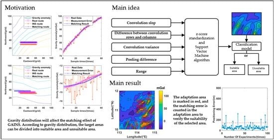
The Sobel operator was used for convolution of the gravity anomaly map, and the convolution slope parameter was constructed. The difference between convolution rows and columns, convolution variance of the feature map, pooling difference, and range parameter of gravity anomaly map was calculated. SVM algorithm was used to fuse these five parameters, and a convolution slope parameter-support vector machine combined method is proposed.

(2)

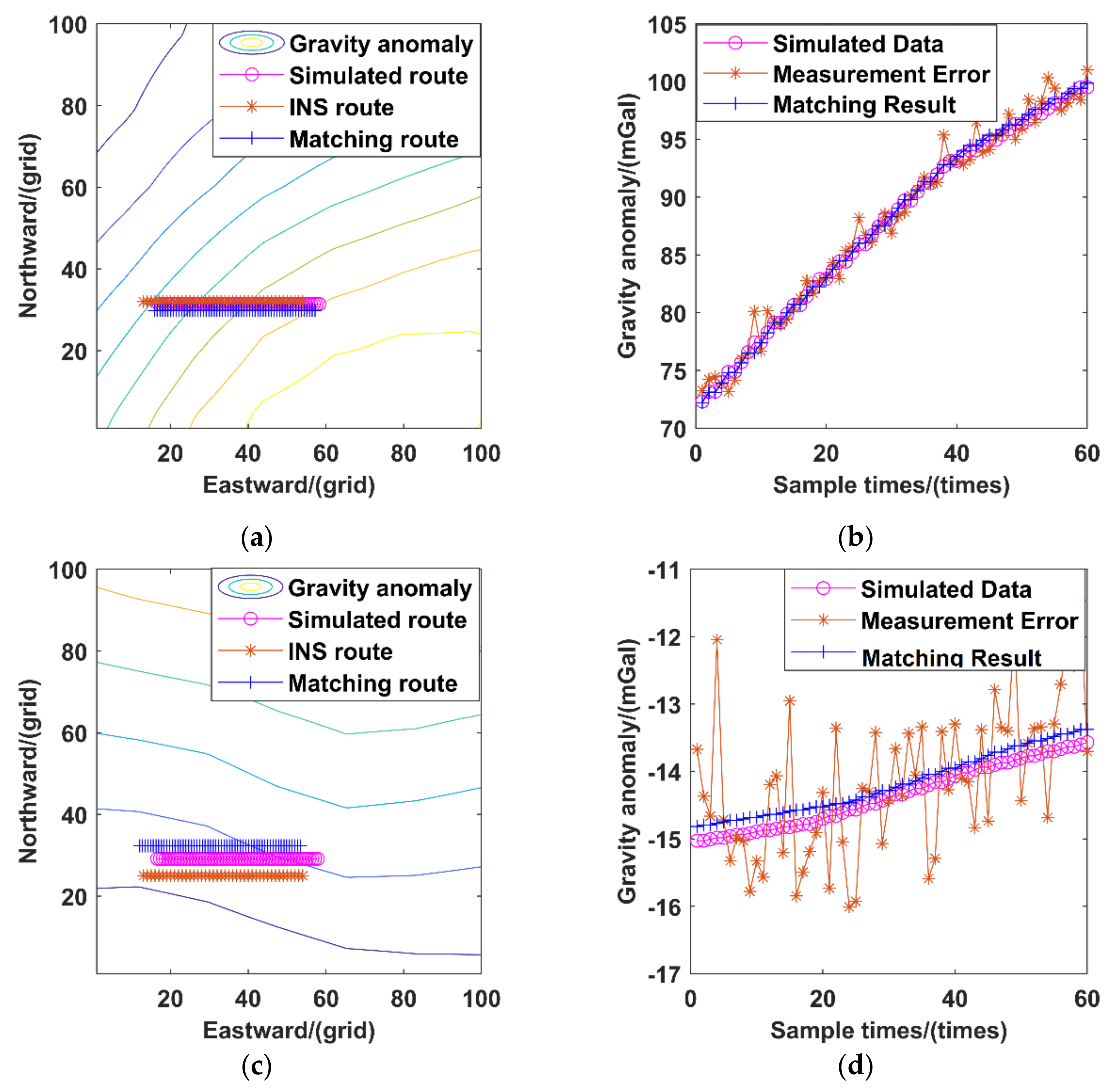
The samples of the target area were divided into the training set and test set. The training set data were used to calculate the classification model, which separates the test-set samples and compares them with the pre-calibration results. In the experimental results, the classification accuracy of the test set is over 92%.

(3)

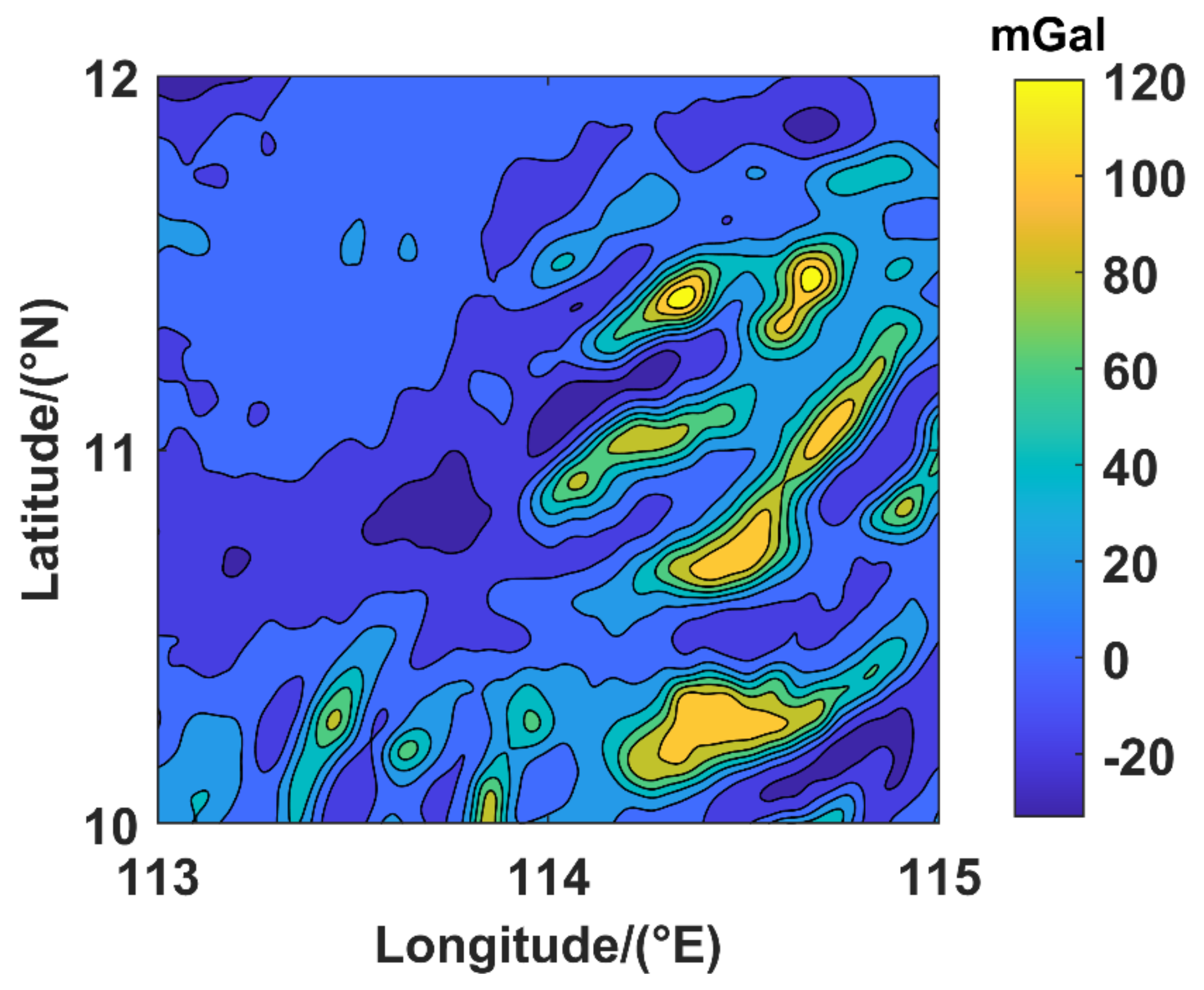
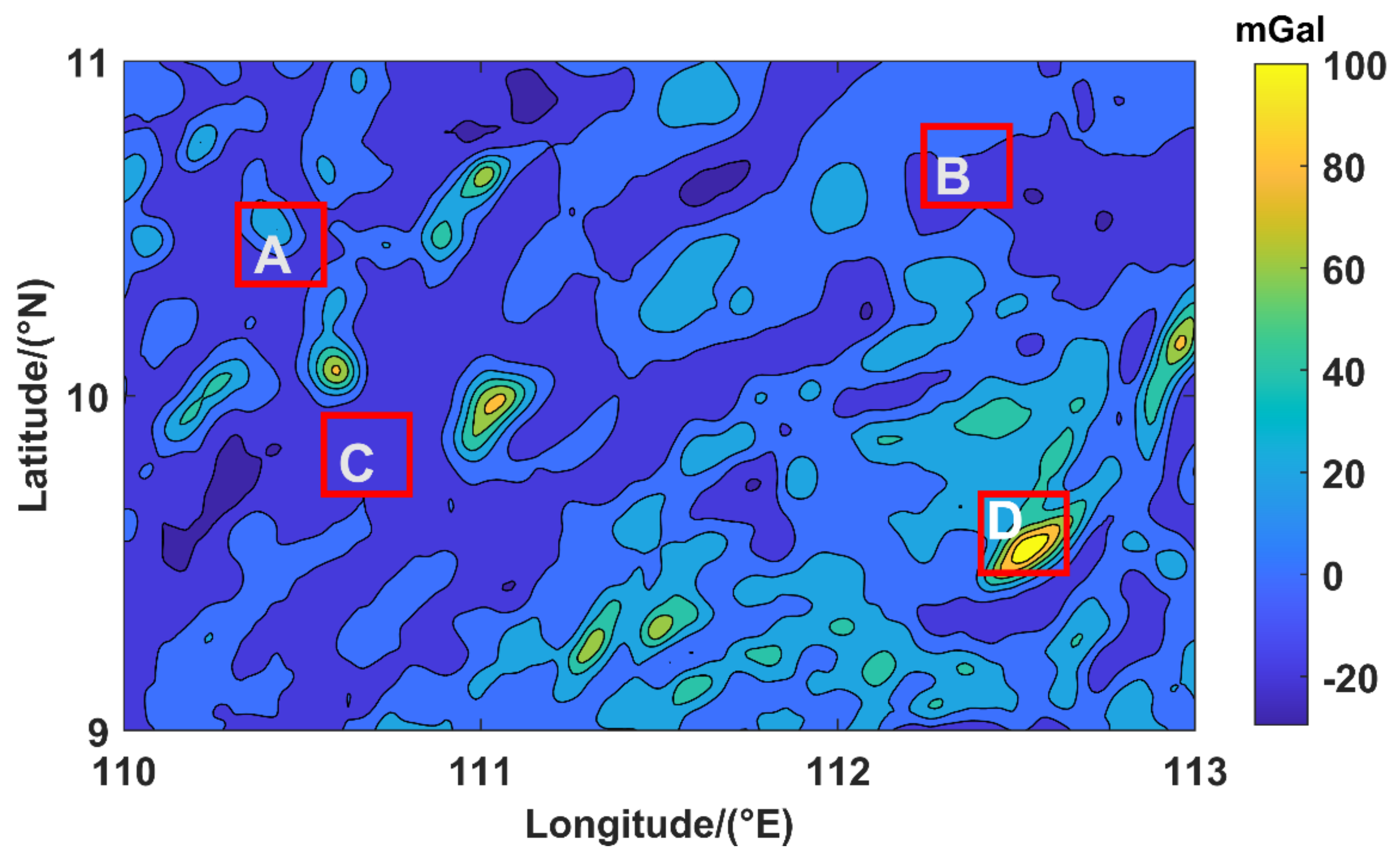
To verify the effectiveness of the classification results, the classification model was applied to another region, and the suitable areas and unsuitable areas were divided. The navigation experiment was carried out in the suitable areas. The results show that the positioning error is better than 100 m, and the accuracy can be more than 91%. It is proven that this method can effectively divide the matching area of GAINS.

References

1. Alamgir, M.S.M.; Sultana, M.N.; Chang, K. Link Adaptation on an Underwater Communications Network Using Machine Learning Algorithms: Boosted Regression Tree Approach. IEEE Access 2020, 8, 73957–73971. [Google Scholar] [CrossRef]
2. Dai, T.; Miao, L.; Shao, H.; Shi, Y. Solving gravity anomaly matching problem under large initial errors in gravity aided navigation by using an affine transformation based artificial bee colony algorithm. Front. Neurorobot. 2019, 13, 19. [Google Scholar] [CrossRef]
3. Han, Y.; Wang, B.; Deng, Z.; Fu, M. A Matching Algorithm Based on the Nonlinear Filter and Similarity Transformation for Gravity-Aided Underwater Navigation. IEEE/ASME Trans. Mechatron. 2018, 23, 646–654. [Google Scholar] [CrossRef]
4. Han, Y.; Wang, B.; Deng, Z.; Wang, S.; Fu, M. A mismatch diagnostic method for TERCOM-Based underwater gravity-aided navigation. IEEE Sens. J. 2017, 17, 2880–2888. [Google Scholar] [CrossRef]
5. Li, Z.; Zheng, W.; Wu, F. Improving the Reliability of Underwater Gravity Matching Navigation Based on a Priori Recursive Iterative Least Squares Mismatching Correction Method. IEEE Access 2020, 8, 8648–8657. [Google Scholar] [CrossRef]
6. Wang, B.; Zhu, J.; Ma, Z.; Deng, Z.; Fu, M. Improved Particle Filter-Based Matching Method with Gravity Sample Vector for Underwater Gravity-Aided Navigation. IEEE Trans. Ind. Electron. 2021, 68, 5206–5216. [Google Scholar] [CrossRef]
7. Wang, K.; Zhu, T.; Qin, Y.; Jiang, R.; Li, Y. Matching error of the iterative closest contour point algorithm for terrain-aided navigation. Aerosp. Sci. Technol. 2018, 73, 210–222. [Google Scholar] [CrossRef]
8. Tang, J.; Xiong, L.; Li, K.; Ma, J. Research on matching area selection based on multiple features fusion of full tensor gravity gradient. MIPPR 2015 Autom. Target Recognit. Navig. 2015, 9812, 98120F. [Google Scholar] [CrossRef]
9. Wang, B.; Zhu, Y.; Deng, Z.; Fu, M. The Gravity Matching Area Selection Criteria for Underwater Gravity-Aided Navigation Application Based on the Comprehensive Characteristic Parameter. IEEE/ASME Trans. Mechatron. 2016, 21, 2935–2943. [Google Scholar] [CrossRef]
10. Wang, H.; Wu, L.; Chai, H.; Xiao, Y.; Hsu, H.; Wang, Y. Characteristics of marine gravity anomaly reference maps and accuracy analysis of gravity matching-aided navigation. Sensors 2017, 17, 1851. [Google Scholar] [CrossRef] [Green Version]
11. Liu, F.; Li, F.; Jing, X. Navigability Analysis of Local Gravity Map With Projection Pursuit-Based Selection Method by Using Gravitation Field Algorithm. IEEE Access 2019, 7, 75873–75889. [Google Scholar] [CrossRef]
12. Wang, B.; Zhou, M.; Deng, Z.; Fu, M. Sum vector-difference-based matching area selection method for underwater gravity-aided navigation. IEEE Access 2019, 7, 123616–123624. [Google Scholar] [CrossRef]
13. Wang, C.; Wang, B.; Deng, Z.; Fu, M. A co-occurrence matrix-based matching area selection algorithm for underwater gravity-aided inertial navigation. IET Radar Sonar Navig. 2021, 15, 250–260. [Google Scholar] [CrossRef]
14. Wang, C.; Wang, B.; Deng, Z.; Fu, M. A delaunay triangulation-based matching area selection algorithm for underwater gravity-aided inertial navigation. IEEE/ASME Trans. Mechatron. 2021, 26, 908–917. [Google Scholar] [CrossRef]
15. Tian, R.; Sun, G.; Liu, X.; Zheng, B. Sobel edge detection based on weighted nuclear norm minimization image denoising. Electronics 2021, 10, 655. [Google Scholar] [CrossRef]
16. Gonzalez, C.I.; Melin, P.; Castro, J.R.; Mendoza, O.; Castillo, O. An improved sobel edge detection method based on generalized type-2 fuzzy logic. Soft Comput. 2016, 20, 773–784. [Google Scholar] [CrossRef]
17. Yildirim, O.; Baloglrf, U.B. Regp: A new pooling algorithm for deep convolutional neural networks. Neural Netw. World 2019, 29, 45–60. [Google Scholar] [CrossRef]
18. Tong, Z.; Tanaka, G. Hybrid pooling for enhancement of generalization ability in deep convolutional neural networks. Neurocomputing 2019, 333, 76–85. [Google Scholar] [CrossRef]
19. Zhang, C.Z.; Feng, H.J.; Xu, Z.H.; Li, Q.; Chen, Y.T. Piecewise noise variance estimation of images based on wavelet transform. J. Zhejiang Univ. Eng. Sci. 2018, 52, 1804–1810. [Google Scholar] [CrossRef]
20. Li, D.G.; Zheng, S. Joint Median and Range Chart with Two-stage Sampling. Math. Pract. Theory 2010, 40, 137–140. [Google Scholar]
21. Singh, D.; Singh, B. Investigating the impact of data normalization on classification performance. Appl. Soft Comput. 2020, 97, 105524. [Google Scholar] [CrossRef]
22. Vapnik, V.; Golowich, S.E.; Smola, A. Support vector method for function approximation, regression estimation, and signal processing. In Advances in Neural Information Processing Systems; Neural Information Processing Systems Foundation: La Jolla, CA, USA, 1997; pp. 281–287. Available online: http://citeseerx.ist.psu.edu/viewdoc/summary?doi=10.1.1.41.3139 (accessed on 15 August 2021).
23. Ju, H.; Hou, Q.; Jing, L. Fuzzy and interval-valued fuzzy nonparallel support vector machine. J. Intell. Fuzzy Syst. 2019, 36, 2677–2690. [Google Scholar] [CrossRef]
24. Ding, S.; Zhu, Z.; Zhang, X. An overview on semi-supervised support vector machine. Neural Comput. Appl. 2017, 28, 969–978. [Google Scholar] [CrossRef]
25. Bazi, Y.; Melgani, F. Toward an optimal SVM classification system for hyperspectral remote sensing images. IEEE Trans. Geosci. Remote Sens. 2006, 44, 3374–3385. [Google Scholar] [CrossRef]
26. Chang, C.C.; Lin, C.J. LIBSVM: A Library for support vector machines. ACM Trans. Intell. Syst. Technol. 2011, 2, 1–27. [Google Scholar] [CrossRef]
Figure 1. The Sobel Operator: (a) horizontal edge-detection operator; (b) vertical edge-detection operator; (c) 45° edge-detection operator; (d) 135° edge-detection operator.
Remotesensing 13 03940 g001
Figure 2. Coverage area of diagonal heading route in target area: (a) Northeast direction; (b) Northwest direction.
Remotesensing 13 03940 g002
Figure 3. Distribution of gravity anomaly in the verification area.
Remotesensing 13 03940 g003
Figure 4. Matching result: (a) routes distribution of suitable area-matching result; (b) gravity anomaly sequence of simulated route and matching route in (a); (c) routes distribution of unsuitable area-matching result; (d) gravity anomaly sequence of simulated route and matching route in (c).
Remotesensing 13 03940 g004
Figure 5. The positioning error of areas A, B, C, and D.
Remotesensing 13 03940 g005
Figure 6. Comparison for pre-calibration and classification results of suitable areas: (a) pre-calibration results of suitable areas for east-west direction; (b) classification results of suitable areas for east-west direction; (c) pre-calibration results of suitable areas for north-south direction; (d) classification results of suitable areas for north-south direction; (e) pre-calibration results of suitable areas for northeast direction; (f) classification results of suitable areas for northeast direction; (g) pre-calibration results of suitable areas for northwest direction; (h) classification results of suitable areas for northwest direction.
Remotesensing 13 03940 g006aRemotesensing 13 03940 g006b
Figure 7. Distribution of gravity anomaly in the application area.
Remotesensing 13 03940 g007
Figure 8. Distribution of suitable areas in application area: (a) suitable areas for east-west direction; (b) suitable areas for north-south direction; (c) suitable areas for northeast direction; (d) suitable areas for northwest direction.
Remotesensing 13 03940 g008aRemotesensing 13 03940 g008b
Figure 9. Positioning error of suitable areas: (a) east-west direction suitable areas; (b) north-south direction suitable area; (c) northeast direction suitable areas; (d) northwest direction suitable areas.
Remotesensing 13 03940 g009