Cross-Dimension Attention Guided Self-Supervised Remote Sensing Single-Image Super-Resolution

Abstract

In recent years, the application of deep learning has achieved a huge leap in the performance of remote sensing image super-resolution (SR). However, most of the existing SR methods employ bicubic downsampling of high-resolution (HR) images to obtain low-resolution (LR) images and use the obtained LR and HR images as training pairs. This supervised method that uses ideal kernel (bicubic) downsampled images to train the network will significantly degrade performance when used in realistic LR remote sensing images, usually resulting in blurry images. The main reason is that the degradation process of real remote sensing images is more complicated. The training data cannot reflect the SR problem of real remote sensing images. Inspired by the self-supervised methods, this paper proposes a cross-dimension attention guided self-supervised remote sensing single-image super-resolution method (CASSISR). It does not require pre-training on a dataset, only utilizes the internal information reproducibility of a single image, and uses the lower-resolution image downsampled from the input image to train the cross-dimension attention network (CDAN). The cross-dimension attention module (CDAM) selectively captures more useful internal duplicate information by modeling the interdependence of channel and spatial features and jointly learning their weights. The proposed CASSISR adapts well to real remote sensing image SR tasks. A large number of experiments show that CASSISR has achieved superior performance to current state-of-the-art methods.

1. Introduction

In the field of remote sensing, HR remote sensing images have rich textures and critical information. They play an important role in remote sensing image analysis tasks such as fine-grained classification [1,2], target recognition [3,4], target tracking [5,6] and land monitoring [7]. However, due to equipment limitations, it is hard to obtain HR remote sensing images. At present, most datasets are composed of LR images instead of HR images. Therefore, image SR technology has shown great potential and has been a research hotspot in recent decades.

Image SR is the process of restoring an HR image from a given LR image. It is a very ill-posed process because multiple HR solutions are mapped to one LR input. Many image SR methods have been proposed to solve this ill-posed problem, including early interpolation-based methods [8], reconstruction-based methods [9], and recent learning-based methods [10,11,12,13].

Recently, image SR methods [10,14,15] based on deep convolutional neural networks (CNN) have made significant progress. For the first time, Dong et al. [10] proposed an SRCNN containing a three-layer convolutional neural network, which achieved better performance than traditional methods. Affected by the residual network (ResNet) [16], VDSR [11] and DRCN [17] increased the network depth to 20 and used a large number of residual structures, and the effect was significantly improved compared to SRCNN. Later, more CNN-based image SR methods [18,19,20] used residual learning strategies. With the introduction of the attention mechanism [21,22], several methods [23,24] began to aggregate the attention mechanism into the SR model, which greatly enhanced the representation ability of static CNN and improved the performance of the image SR network.

These deep learning-based methods [11,17,20] design a very deep and complex CNN and train it for a long time (days or weeks) through a large number of high-quality external datasets. Most of these kinds of external datasets use fixed bicubic downsampling operations to construct training data pairs, such as the DIV2K [25] dataset. Similarly, the input image in the test phase is still obtained by bicubic core downsampling. However, real LR remote sensing images do not meet these conditions. In this ‘non-ideal’ situation, these supervised methods often produce poor results. The main reason is that the bicubic downsampled image cannot reflect the degradation process of the real LR image.

Inspired by many unsupervised image enhancement methods [26,27,28,29,30,31,32,33] and attention mechanism model [21,22], in this paper, we introduce cross-dimension attention guided self-supervised remote sensing single-image super-resolution method (CASSISR). The CASSISR does not require pre-training on a dataset, uses the internal reproducibility of the internal information of a single image, and merely utilizes the lower-resolution images extracted from the input image itself to train the attention guided convolutional network. Therefore, the CASSISR has great advantages in ‘non-ideal’ situations.

The cross-scale recurrence of small pieces of information in a single image has proven to be a very powerful feature of natural images [26,34]. Through our research, we found that the cross-scale repetition of internal information in remote sensing images is more powerful than natural images. As shown in Figure 1, the small-scale information in the red frame can be found in other places within the same picture (large-scale information in the blue frame). The CASSISR takes advantage of the cross-scale internal reproducibility of image-specific information and trains attention guided convolutional networks with LR images and their downsampled lower-resolution images to infer the LR–HR relationship. Then, the trained network is applied to the LR input image to produce the SR output.

In order to better learn the cross-scale information within the image and improve the performance of the image SR network, we propose a cross-dimension attention mechanism module (CDAM). Different from SENet [21] and CBAM [22], we consider the interactivity between the channel dimension and the spatial dimension by modeling the interdependence of the channel and the spatial feature, jointly learning the feature weight of the channel and spatial, and selectively capturing more useful internal duplicate information. In order to verify the validity of CASSISR, we construct the ‘ideal’ remote sensing dataset, ‘non-ideal’ remote sensing dataset, and real-world remote sensing dataset. We conduct a lot of experiments on these three types of datasets. Although the effect of CASSISR on the ‘ideal’ remote sensing dataset does not exceed that of the supervised SOTA-SR methods, the generated results are still surprising, even if CASSISR only trains through one image. However, for the ‘non-ideal’ remote sensing dataset and real-world remote sensing dataset, CASSISR greatly exceeds the SOTA-SR methods, and the visual effects also have obvious advantages.

In summary, our contributions in this paper are summarized as follows:

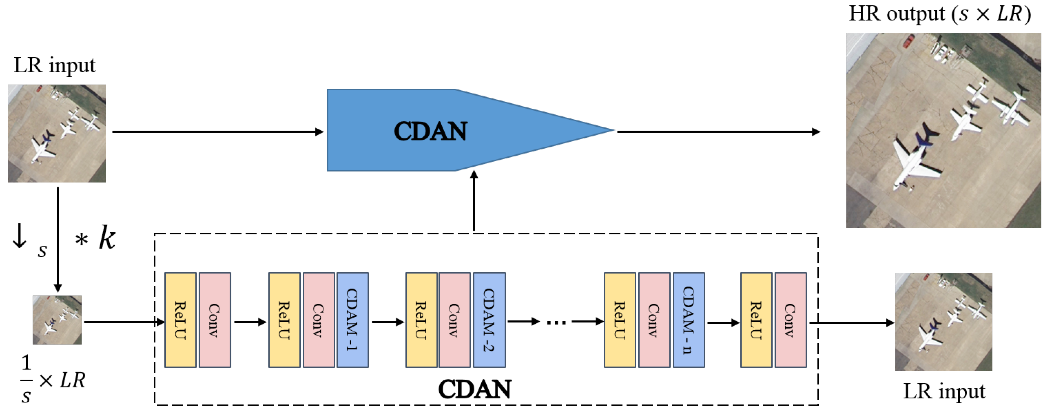
• We introduce a cross-dimension attention guided self-supervised remote sensing single-image super-resolution method (CASSISR). Our CASSISR only needs one image for training. It takes advantage of the reproducibility of the internal information of a single image, does not require prior training in the dataset, and only uses the lower-resolution images extracted from a single input image itself to train the attention guided convolutional network (CDAN), which can better adapt to real remote sensing image super-resolution tasks.
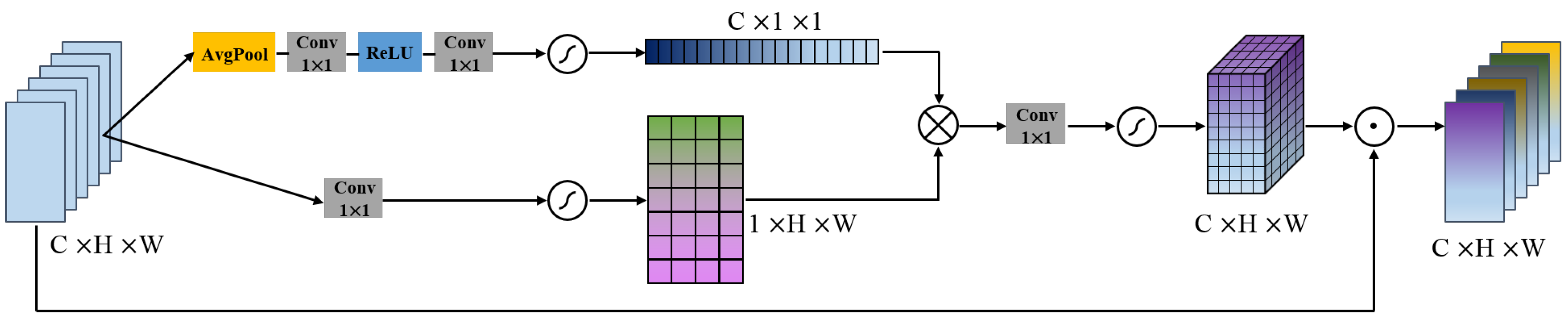
• We propose a cross-dimension attention mechanism module (CDAM). It considers the interaction between the channel dimension and the spatial dimension by modeling the interdependence between the channel and the spatial feature, jointly learning the feature weight of the channel and the spatial, selectively capturing more useful internal duplicate information, improving the learning ability of static CNN.
• We conduct a large number of experiments on the ‘ideal’ remote sensing dataset, ‘non-ideal’ remote sensing dataset, and real-world remote sensing dataset, and compare the experimental results with the SOTA-SR methods. Although there is only one training image for CASSISR, it still obtains more favorable results.

2. Related Work

After the efforts of a large number of researchers, the computer vision community has proposed a large number of image SR methods, including interpolation-based methods [8], reconstruction-based methods [9], and CNN-based methods [10,11]. This section briefly reviewed the related work of the CNN-based SR methods, remote sensing SR methods, and attention mechanisms.

2.1. CNN-Based SR Method

Recently, CNN-based SR networks have been extensively studied. As a pioneering work, Dong et al. [10] propose a shallow three-layer convolutional network (SRCNN) for image SR and achieves satisfactory performance. They use bicubic interpolation to enlarge the LR image to the target size and then adopt a three-layer convolutional network to fit the non-linear mapping. Subsequently, Kim et al. [11] introduce the residual structure and design a VDSR model with a deeper network structure so that the model has a wider receptive field. Dong et al. [35] directly learn the mapping of LR images to HR images by using deconvolution in FSRCNN. To further improve the performance, Lim et al. [18] propose a deep and wide network EDSR composed of the remaining blocks modified by stacking and removed the batch normalization (BN) layer. Zhang et al. [15] utilize all hierarchical features of all convolutional layers in RDN through dense connections.

2.2. Remote Sensing SR Method

SR algorithms based on deep learning have also been applied to SR tasks in the field of remote sensing. Inspired by VDSR [11], Huang et al. [36] propose a remote sensing deep residual learning network RS-DRL. Lei et al. [37] propose a ‘Multi-Fork’ CNN architecture for training in an end-to-end manner. Xu et al. [38] introduce a new deep memory connection network (DMCN), which reduces the time required to reconstruct the resolution of remote sensing images. Gu et al. [39] use residual squeeze and excitation blocks to model the dependence among channels, which improves the representation ability. Wang et al. [40] propose an adaptive multi-scale feature fusion network and use sub-pixel convolution for image reconstruction. However, these remote sensing SR methods require long-term training through a large number of synthetic external datasets, and it is difficult to adapt to real-world LR remote sensing images.

2.3. Attention Mechanism

In recent years, the attention mechanism has been widely used in various computer vision tasks and has become an essential part of the neural network structure. Jaderberg et al. [41] propose for the first time an effective spatial attention mechanism (STN) that can locate the target and learn the corresponding deformation and then preprocess it to reduce the difficulty of model learning. Hu et al. [21] introduce an effective channel attention learning mechanism (SENet), which models the importance of each feature channel to enhance or suppress the importance of different channels for different tasks. Gao et al. [42] introduce GSoP and introduce a second-order pool to achieve more effective functional aggregation. Hu et al. [43] use deep convolution to explore spatial expansion to gather features. Woo et al. [22] propose CBAM, which uses average pooling and maximum pooling to aggregate features, and combines channel attention and spatial attention. Introducing the attention mechanism into the SR model further improves the SR performance [23]. However, these attention models model independently in the spatial dimension or the channel dimension, ignoring the interaction between the channel dimension and the spatial dimension.

3. Materials and Methods

In this section, we first introduce the overall overview of cross-dimension attention guided self-supervised remote sensing single-image super-resolution (CASSISR). Then we give the detailed structure of the proposed cross-dimension attention mechanism module (CDAM). Finally, we introduce the loss function and parameter settings of the network.

3.1. Overall Network Overview

The LR image can be assumed to be the result of convolution downsampling of the HR image and the blur kernel $\mathit{k}$ and adding noise $\mathit{n}$. The relationship between the LR image and HR image can be modeled as:

$$I_{LR}=(I_{HR}\ast k){\downarrow }_s+ n$$

(1)

where $I_{LR}$ denotes the LR image, $I_{HR}$ denotes the HR image, ∗ denotes the convolution operation, k denotes the blur kernel, ${\downarrow }_s$ denotes the downsampling with a scale factor of s and n denotes the noise. For the SR of real-world remote sensing images, $I_{HR}$ is unknown, and k and n are also not fixed. It is unreasonable for the supervised CNN-based SR methods to use fixed bicubic downsampling to construct the training data pair. These methods ideally model the relationship between the LR image and SR image:

$$I_{LR}=I_{HR}{\downarrow }_s$$

(2)

where $I_{LR}$ and $I_{HR}$ represent the LR and HR image, respectively, and ${\downarrow }_s$ represents the downsampling with a scale factor of s. This kind of network trained on a large number of ideal datasets will certainly generate better results when used for images that have also been downsampled by the bicubic kernel. However, when the input is a real-world image or an image that is not bicubic downsampled, the generated result will be blurry. The LR images of this ideal bicubic downsampling structure do not conform to the complex situation of the real-world LR images. Therefore, in the case of real-world SR, there is only one original LR image. How can we solve this problem?

We mainly use the powerful internal information repetitiveness of remote sensing images. In the same remote sensing image, specific information will repeatedly appear at different scales and positions. Therefore, the CASSISR does not require prior training on paired datasets and only requires a given single low-resolution image as input. Figure 2 shows the overall network structure. Given a low-resolution input image $\mathit{LR}$, a lower-resolution image obtained by reducing the scale of the image $\mathit{LR}$ is $\frac{1}{s}\times LR$ (where $\mathit{s}$ is the super-resolution scale factor). We design a cross-dimension attention network (CDAN) and train it to reconstruct the input low-resolution image $\mathit{LR}$ from the lower-resolution image $\frac{1}{s}\times LR$. Then, we use the image LR as the input of the trained CDAN to generate the required high-resolution image $\mathit{HR}$ ($\mathit{HR}=\mathit{s}\times \mathit{LR}$). The cross-dimension attention network can better capture the non-local features of the image and improve the learning ability of the network. Among them, CDAM is the proposed cross-dimension attention module, which we will introduce in detail in the next section.

3.2. Cross-Dimension Attention Module

The existing channel attention mechanism mainly focuses on channel dimension information and ignores the spatial dimension information, while the spatial attention mechanism ignores the channel dimension information. These models do not consider the interactivity between the channel dimension and the spatial dimension. To solve this problem, we propose a cross-dimension attention module (CDAM), which can selectively capture more useful internal duplicate information by modeling the interdependence of channel and spatial features, and jointly learning the feature weights of the channel and spatial. The structure of the proposed CDAM is shown in Figure 3.

Suppose that the feature maps $\mathit{F}\in {\mathbb{R}}^{C\times H\times W}$ are the input of CDAM, $\mathit{C}$ is the number of channels, $\mathit{H}$ and $\mathit{W}$ are the height and the width of the feature maps, respectively. We use global average pooling to compress the global spatial information into a channel descriptor, and then obtain the weight matrix ${\mathit{T}}_{\mathit{c}}\in {\mathbb{R}}^{C\times 1\times 1}$ of different channel information through the convolutional layer, Relu and sigmoid activation functions. We obtain the weight matrix ${\mathit{T}}_{\mathit{s}}\in {\mathbb{R}}^{1\times H\times W}$ of different spatial information through the convolutional layer and the sigmoid activation function. Then we matrix multiply the channel information weight matrix and the spatial information weight matrix, and then obtain the cross-scale channel spatial attention weight $\mathit{T}\in {\mathbb{R}}^{C\times H\times W}$ through the convolutional layer and the sigmoid activation function. Finally, the cross-dimension channel-spatial attention weight $\mathit{T}$ and the input feature $\mathit{F}$ are subjected to element-wise multiplication to obtain a weighted feature map $\tilde{\mathit{F}}\in {\mathbb{R}}^{C\times H\times W}$. The cross-dimension attention module can be formulated as follows:

$${\mathit{T}}_{\mathit{c}}=Sigmoid\left(f^{1\times 1}\left(ReLU\left(f^{1\times 1}\left(Avg\left(\mathit{F}\right)\right)\right)\right)\right)$$

(3)

$${\mathit{T}}_{\mathit{s}}=Sigmoid\left(f^{1\times 1}\left(\mathit{F}\right)\right)$$

(4)

$$\tilde{\mathit{F}}=\left(Sigmoid\left(f^{1\times 1}({\mathit{T}}_{\mathit{c}}\otimes {\mathit{T}}_{\mathit{s}})\right)\right)\odot \mathit{F}$$

(5)

where $\mathit{Avg}$ is the global average pooling, $f^{1\times 1}$ is the convolution operation with a filter size of $1\times 1$, ⊗ is the matrix multiplication and ⊙ is the element-wise multiplication. Different from the previous spatial attention and channel attention [21,22,44], we model the cross-dimension interdependence of channel and spatial feature information through jointly learning channel and spatial feature weights and the mutual influence and interdependence between channels and spatial features to learn the channel-spatial attention weight better.

3.3. Network Settings and Loss Function

Because the training of a single image does not require a deep and complex network, we set the number of cross-dimension attention modules (CDAM) of the cross-dimension attention network (CDAN) to only 6. We use the Adam optimizer [45], where the learning rate starts from $0.0001$, and the reconstruction error is linearly fitted periodically. When the standard deviation is greater than the slope of the linear fitting, the learning rate is divided by 10, and training is stopped when the learning rate reaches ${10}^{-6}$. At the same time, we also enhance the data by rotating ($0^{\circ }$, ${90}^{\circ }$, ${180}^{\circ }$, ${270}^{\circ }$) and specular reflection in the vertical and horizontal directions. We use the ${\mathit{L}}_1$ loss function to minimize the error between the true value and the predicted value and optimize the ${\mathit{L}}_1$ loss.

$$L_1\left(\theta \right)=\sum _{i=1}^n|LR-\mathrm{CDAN}(\frac{1}{s}\times LR)|$$

(6)

where $\theta$ is the CDAN parameter, $\mathit{LR}$ is the input low-resolution image, and $\frac{1}{s}\times LR$ is the lower-resolution image obtained by reducing the $\mathit{s}$ times scale of the image $\mathit{LR}$.

4. Results

In this section, we first introduce the ‘ideal’ remote sensing dataset, the ‘non-ideal’ remote sensing dataset, and the real-world remote sensing dataset. Then we conduct experiments on these three types of datasets to compare the CASSISR with existing algorithms. For ‘ideal’ remote sensing dataset and ‘non-ideal’ remote sensing dataset, we use PSNR and SSIM as metrics to quantitatively compare the CASSISR algorithm with existing algorithms and show the visualization results. Because the real-world remote sensing dataset has no real images of the ground truth for reference in the testing stage, we only show the qualitative results of visual comparison.

4.1. Datasets Construction

4.1.1. ‘Ideal’ Remote Sensing Dataset

We randomly select images from 6 remote sensing datasets (i.e., RSSCN7 dataset [46], RSC11 dataset [47], WHU-RS19 dataset [48], UC-Merced dataset [49], AID dataset [50], and NWPU45 dataset [51]) according to categories, and then LR images obtained by bicubic downsampling to form an ‘ideal’ remote sensing dataset.

RSSCN7 dataset [46]: This dataset contains 2800 aerial scene images in 7 typical scene categories (i.e., grassland, forest, farmland, parking lot, residential area, industrial area, river, and lake). The size of each image is $400\times 400$ pixels. We randomly select 10 images from each category, obtain LR images through bicubic downsampling, and use these 70 images as the test dataset.

RSC11 dataset [47]: This dataset covers high-resolution remote sensing images of several American cities, including Washington D.C., Los Angeles, San Francisco, New York, San Diego, Chicago, and Houston, including 1232 images of 11 complex scene categories, such as forests, grasslands, ports, tall buildings, low buildings, overpasses, railways, residential areas, roads, sparse forests, and storage tanks. The size of each image is $512\times 512$ pixels. We randomly select 10 images from each category, obtain LR images through bicubic downsampling and use these 110 images as the test dataset.

WHU-RS19 dataset [48]: This dataset consists of 1005 images in 19 different scene categories, including airports, beaches, bridges, commercial areas, deserts, farmland, football fields, forests, industrial areas, grasslands, mountains, parks, parking lots, etc. The size of each image is $600\times 600$ pixels. We randomly select 10 images from each category, obtain LR images through bicubic downsampling and use these 190 images as the test dataset.

UC-Merced dataset [49]: This dataset consists of 2100 images in 21 land use categories, including agriculture, airplanes, baseball fields, beaches, buildings, small churches, etc. The size of each image is $256\times 256$ pixels. We randomly select 10 images from each category, obtain LR images through bicubic downsampling and use these 210 images as the test dataset.

AID dataset [50]: This dataset consists of 10,000 images in 30 aerial scene categories, including airports, bare ground, baseball fields, beaches, bridges, centers, churches, commercials, dense residences, deserts, farmlands, forests, etc. The size of each image is $600\times 600$ pixels. We randomly select 10 images from each category, obtain LR images through bicubic downsampling and use these 300 images as the test dataset.

NWPU45 dataset [51]: This dataset consists of 31,500 images of 45 scene categories, including airport, baseball diamond, basketball court, beach, bridge, chaparral, church, etc. The size of each image is $256\times 256$ pixels. We randomly select 10 images from each category, obtain LR images through bicubic downsampling and use these 450 images as the test dataset.

4.1.2. ‘Non-Ideal’ Remote Sensing Dataset

To better simulate the situation of real-world remote sensing images, we use randomly generated anisotropic Gaussian kernels to blur and downsample the above 6 datasets [52]. The size of the kernels is $11\times 11$, with random lengths ${\lambda }_1,{\lambda }_2\sim \mu (0.6,5)$ distributed independently on each axis, rotated by a random angle $\theta \sim \mu [-\pi ,\pi ]$. In this way, we constructed a ‘non-ideal’ remote sensing datasets, including RSSCN7-blur dataset, RSC11-blur dataset, WHU-RS19-blur dataset, UC-Merced-blur dataset, AID-blur dataset, and NWPU45-blur dataset, which are closer to real LR images.

4.1.3. Real-World Remote Sensing Dataset

To better reflect the advantages of CASSISR, we directly extract the original images from the OSCD dataset [53] as the real remote sensing dataset. This dataset includes 24 pairs of multispectral images taken from the Sentinel-2 satellite between 2015 and 2018, including Brazil, the United States, Europe, the Middle East, and Asia. The spatial resolution of the image is between 10, 20, and 60 m, with different sizes. Since there is no ground truth for reference during the verification phase, we only show the results of the visual comparison.

4.2. Experiments on ‘Ideal’ Remote Sensing Dataset

Research on the ‘ideal’ remote sensing dataset is not our research focus, but we still compare CASSISR with CNN-based SR methods and remote sensing SR methods. As shown in

Table 1. The quantitative results of CASSISR, CNN-based SR methods, and remote sensing SR methods on the ‘ideal’ remote sensing dataset (bicubic downsampling). Our CASSISR results are highlighted, and the best results are underlined. Please note that CASSISR only uses one image for training, while other methods are trained on large datasets.

Method	Scale	RSSCN7	RSC11	WHU-RS19	UC-Merced	AID	NWPU45
		PSNR/SSIM	PSNR/SSIM	PSNR/SSIM	PSNR/SSIM	PSNR/SSIM	PSNR/SSIM
Bicubic	$\times 2$	$31.26$/$0.8595$	$30.55$/$0.8501$	$34.70$/$0.9216$	$31.74$/$0.8872$	$34.63$/$0.9068$	$31.38$/$0.8741$
SRCNN [10]	$\times 2$	$32.74$/$0.8982$	$32.12$/$0.8915$	$36.04$/$0.9497$	$33.85$/$0.9238$	$35.94$/$0.9367$	$33.03$/$0.9128$
FSRCNN [35]	$\times 2$	$32.90$/$0.9007$	$32.28$/$0.8946$	$36.37$/$0.9521$	$34.29$/$0.9288$	$36.24$/$0.9392$	$33.27$/$0.9160$
EDSR [18]	$\times 2$	$33.51$/$0.9082$	$33.15$/$0.9050$	$37.73$/$0.9572$	$35.61$/$0.9391$	$37.48$/$0.9451$	$33.96$/$0.9231$
SRMD [12]	$\times 2$	$33.37$/$0.9063$	$32.71$/$0.9008$	$37.41$/$0.9553$	$35.09$/$0.9347$	$37.23$/$0.9431$	$33.77$/$0.9210$
RDN [15]	$\times 2$	$33.50$/$0.9089$	$33.19$/$0.9060$	$37.54$/$0.9577$	$35.65$/$0.9405$	$37.31$/$0.9455$	$33.95$/$0.9238$
RCAN [23]	$\times 2$	$33.68$/$0.9107$	$33.42$/$0.9081$	$38.01$/$0.9592$	$36.03$/$0.9426$	$\underline{37.70}$/$\underline{0.9469}$	$34.16$/$0.9256$
SAN [13]	$\times 2$	$\underline{33.72}$/$\underline{0.9115}$	$\underline{33.48}$/$\underline{0.9087}$	$\underline{38.18}$/$\underline{0.9599}$	$36.01$/$0.9424$	$37.69$/$0.9468$	$34.37$/$0.9286$
CS-NL [54]	$\times 2$	$33.68$/$0.9105$	$33.41$/$0.9076$	$37.98$/$0.9589$	$\underline{36.06}$/$\underline{0.9429}$	$37.68$/$0.9467$	$34.13$/$0.9252$
LGCNet [37]	$\times 2$	$--$/$--$	$--$/$--$	$--$/$--$	$33.80$/$0.8917$	$--$/$--$	$32.86$/$0.8788$
DMCN [38]	$\times 2$	$--$/$--$	$--$/$--$	$--$/$--$	$34.19$/$0.8941$	$--$/$--$	$33.07$/$0.8842$
DRSEN [39]	$\times 2$	$--$/$--$	$--$/$--$	$--$/$--$	$34.79$/$0.9470$	$--$/$--$	$34.40$/$0.9385$
DCM [40]	$\times 2$	$--$/$--$	$--$/$--$	$--$/$--$	$33.65$/$0.9274$	$--$/$--$	$--$/$--$
AMFFN [55]	$\times 2$	$--$/$--$	$--$/$--$	$--$/$--$	$35.00$/$0.9360$	$--$/$--$	$\underline{35.30}$/$\underline{0.9348}$
CASSISR(Our)	$\times 2$	$\mathbf{33}.\mathbf{01}$/$\mathbf{0}.\mathbf{9027}$	$\mathbf{32}.\mathbf{23}$/$\mathbf{0}.\mathbf{8956}$	$\mathbf{36}.\mathbf{69}$/$\mathbf{0}.\mathbf{9514}$	$\mathbf{34}.\mathbf{21}$/$\mathbf{0}.\mathbf{9261}$	$\mathbf{36}.\mathbf{64}$/$\mathbf{0}.\mathbf{9399}$	$\mathbf{33}.\mathbf{23}$/$\mathbf{0}.\mathbf{9153}$
Bicubic	$\times 4$	$27.36$/$0.6794$	$26.48$/$0.6509$	$28.93$/$0.7468$	$26.50$/$0.6968$	$29.31$/$0.7442$	$26.90$/$0.6851$
SRCNN [10]	$\times 4$	$28.11$/$0.7203$	$27.23$/$0.6937$	$29.84$/$0.7913$	$27.67$/$0.7464$	$30.16$/$0.7827$	$27.82$/$0.7321$
FSRCNN [35]	$\times 4$	$28.20$/$0.7238$	$27.31$/$0.6979$	$29.81$/$0.7928$	$27.81$/$0.7509$	$30.23$/$0.7855$	$27.93$/$0.7367$
EDSR [18]	$\times 4$	$28.74$/$0.7452$	$27.86$/$0.7249$	$30.66$/$0.8159$	$28.81$/$0.7869$	$31.08$/$0.8084$	$28.52$/$0.7615$
SRMD [12]	$\times 4$	$28.63$/$0.7407$	$27.72$/$0.7184$	$30.57$/$0.8124$	$28.53$/$0.7764$	$30.93$/$0.8034$	$28.40$/$0.7563$
RDN [15]	$\times 4$	$28.77$/$0.7471$	$27.87$/$0.7272$	$30.67$/$0.8177$	$28.91$/$0.7917$	$31.10$/$0.8106$	$28.55$/$0.7637$
RCAN [23]	$\times 4$	$28.87$/$0.7510$	$27.98$/$0.7329$	$30.83$/$0.8218$	$29.14$/$0.7988$	$31.26$/$0.8146$	$28.68$/$0.7689$
SAN [13]	$\times 4$	$28.90$/$0.7503$	$\underline{28.08}$/$\underline{0.7338}$	$\underline{30.96}$/$\underline{0.8233}$	$29.20$/$0.7993$	$\underline{31.34}$/$\underline{0.8150}$	$28.74$/$0.7689$
CS-NL [54]	$\times 4$	$\underline{28.92}$/$\underline{0.7508}$	$28.01$/$0.7305$	$30.91$/$0.8218$	$\underline{29.38}$/$\underline{0.8041}$	$31.30$/$0.8135$	$28.71$/$0.7674$
LGCNet [37]	$\times 4$	$--$/$--$	$--$/$--$	$--$/$--$	$27.40$/$0.5963$	$--$/$--$	$27.35$/$0.5633$
DMCN [38]	$\times 4$	$--$/$--$	$--$/$--$	$--$/$--$	$27.57$/$0.6150$	$--$/$--$	$27.52$/$0.5858$
DRSEN [39]	$\times 4$	$--$/$--$	$--$/$--$	$--$/$--$	$28.14$/$0.8153$	$--$/$--$	$28.54$/$0.7846$
DCM [40]	$\times 4$	$--$/$--$	$--$/$--$	$--$/$--$	$27.22$/$0.7528$	$--$/$--$	$--$/$--$
AMFFN [55]	$\times 4$	$--$/$--$	$--$/$--$	$--$/$--$	$28.70$/$0.7772$	$--$/$--$	$\underline{29.47}$/$\underline{0.7763}$
CASSISR(Our)	$\times 4$	$\mathbf{27}.\mathbf{99}$/$\mathbf{0}.\mathbf{7163}$	$\mathbf{27}.\mathbf{13}$/$\mathbf{0}.\mathbf{6913}$	$\mathbf{29}.\mathbf{78}$/$\mathbf{0}.\mathbf{7868}$	$\mathbf{27}.\mathbf{26}$/$\mathbf{0}.\mathbf{7334}$	$\mathbf{30}.\mathbf{19}$/$\mathbf{0}.\mathbf{7813}$	$\mathbf{27}.\mathbf{53}$/$\mathbf{0}.\mathbf{7216}$

, we report the quantitative comparison results of the scale factors $\times 2$ and $\times 4$ on the ‘ideal’ remote sensing image dataset. Among them, SRCNN [10], FSRCNN [35], EDSR [18], SRMD [12], RDN [15], RCAN [23], SAN [13], and CS-NL [54] are CNN-based SR methods, and LGCNet [37], DMCN [38], DRSEN [39], DCM [40], and AMFFN [55] are remote sensing SR methods. The result of the CNN-based SR methods is tested with the pre-trained model of the DIV2K [25] dataset. For remote sensing SR methods, we directly use the results given in the original paper, and these methods are also pre-trained through a large number of synthetic datasets. However, our CASSISR has not been pre-trained with a large number of datasets.

On the ‘ideal’ remote sensing dataset, even if CASSISR does not exceed the advanced CNN-based and remote sensing SR methods, it is better than the early methods. This is because advanced SR methods use deeper and more complex networks, requiring long-term training, which will take up a lot of computing resources. These methods can indeed show excellent on the ideal bicubic downsampled LR image, but they are not suitable for real remote sensing image SR.

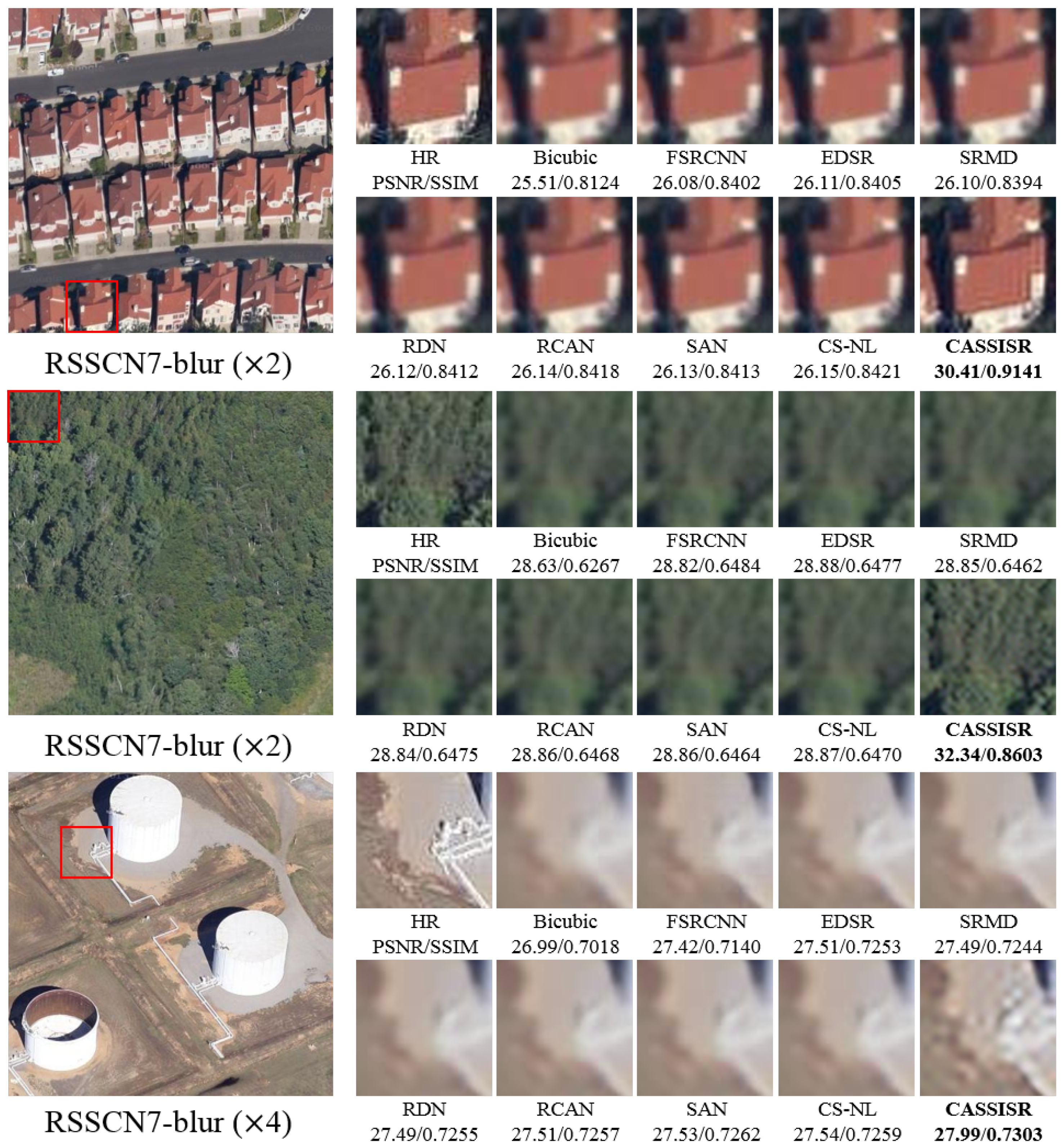
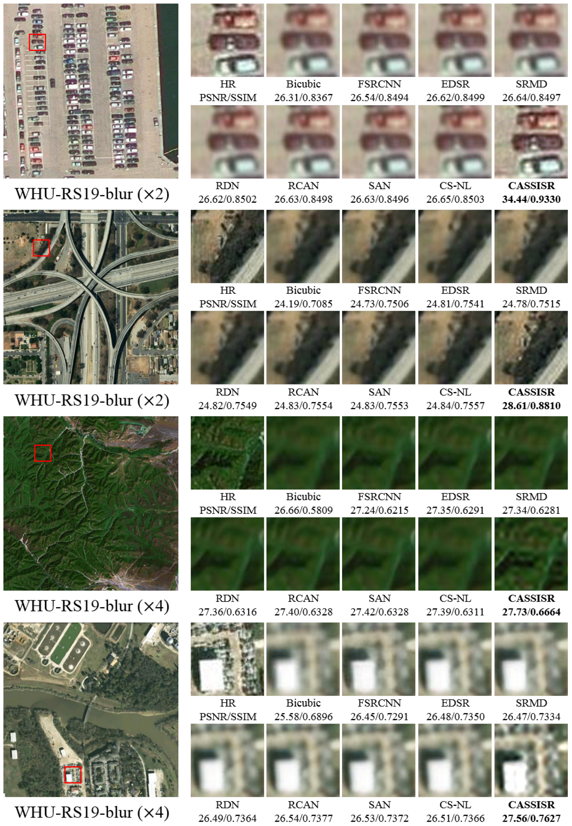
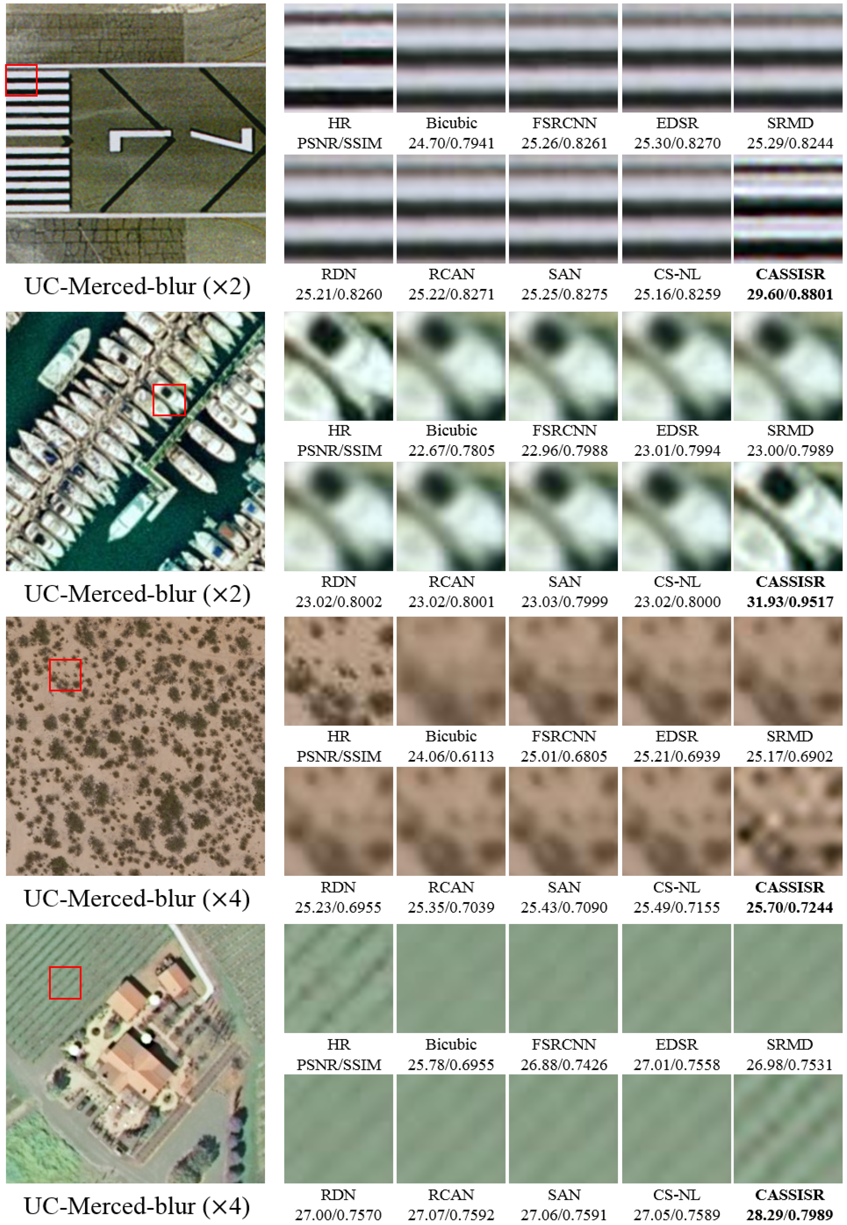
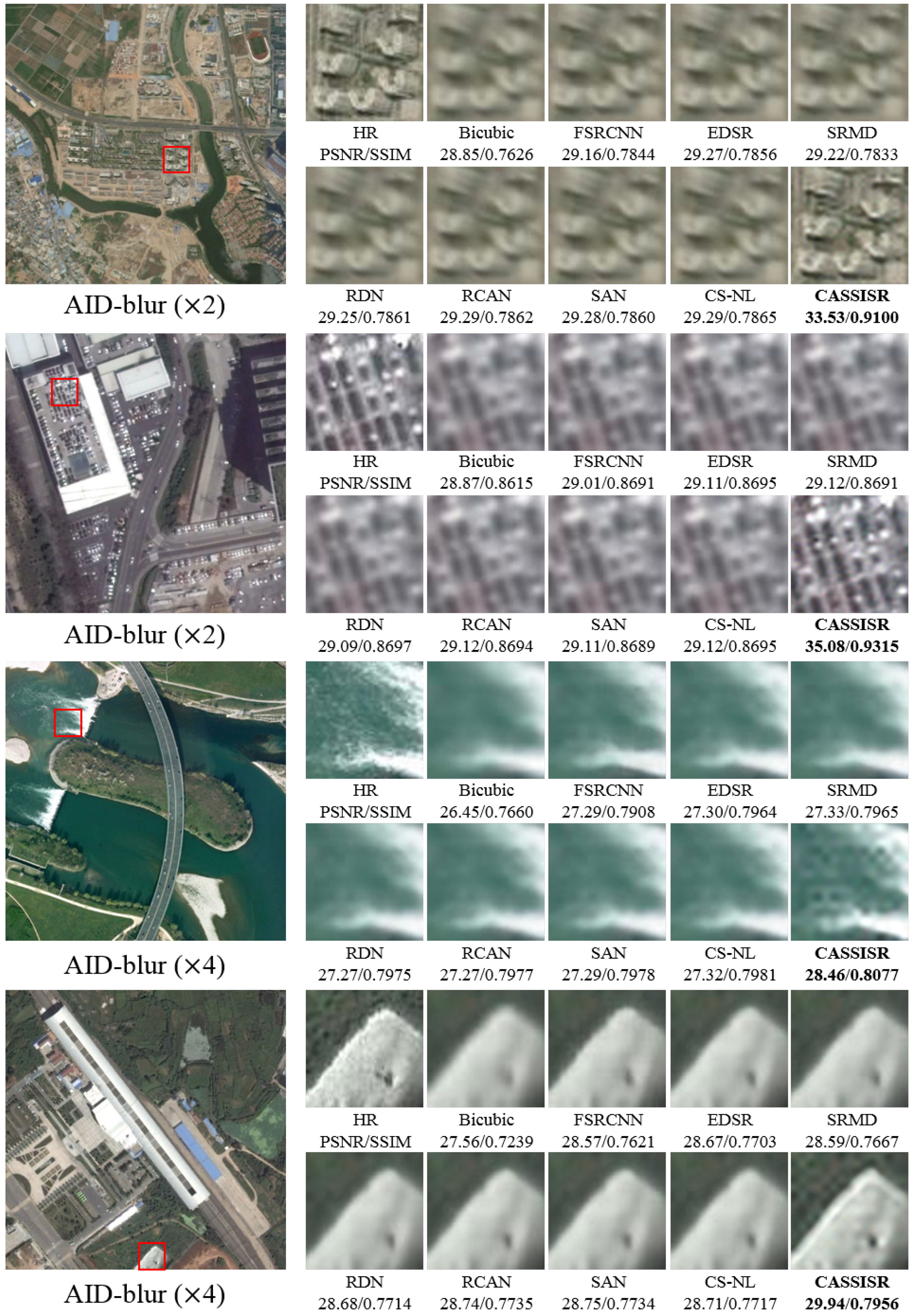
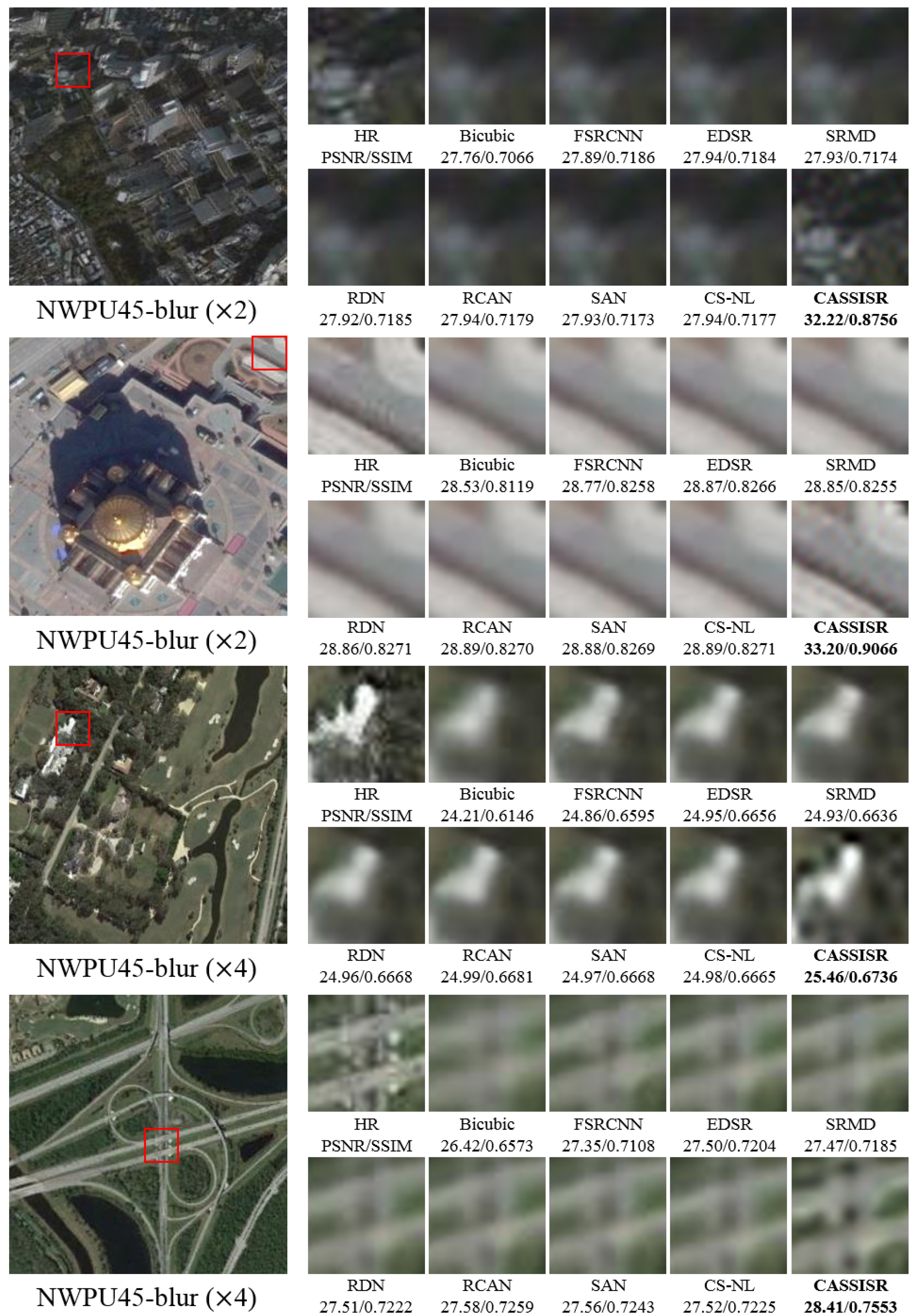
4.3. Experiments on ‘Non-Ideal’ Remote Sensing Dataset

The ‘non-ideal’ remote sensing dataset can better simulate the complex situation of real remote sensing images. We compared CASSISR with CNN-based SR methods quantitatively and qualitatively. The result of the CNN-based SR methods is tested with the pre-trained model.

4.3.1. Quantitative Results

As shown in

Table 2. The quantitative results of CASSISR and CNN-based SR methods on a ‘non-ideal’ remote sensing dataset (random Gaussian kernel downsampling). Our CASSISR results are highlighted, and the best results are underlined. Our CASSISR performs the best.

Method	Scale	RSSCN7-Blur	RSC11-Blur	WHU-RS19-Blur	UC-Merced-Blur	AID-Blur	NWPU45-Blur
		PSNR/SSIM	PSNR/SSIM	PSNR/SSIM	PSNR/SSIM	PSNR/SSIM	PSNR/SSIM
Bicubic	$\times 2$	$27.69$/$0.7133$	$26.86$/$0.6920$	$29.06$/$0.7771$	$26.78$/$0.7354$	$29.30$/$0.7704$	$27.07$/$0.7149$
SRCNN [10]	$\times 2$	$27.86$/$0.7311$	$27.09$/$0.7121$	$29.08$/$0.7936$	$27.01$/$0.7548$	$29.36$/$0.7865$	$27.32$/$0.7348$
FSRCNN [35]	$\times 2$	$27.87$/$0.7313$	$27.11$/$0.7128$	$28.96$/$0.7869$	$27.04$/$0.7559$	$29.48$/$0.7891$	$27.33$/$0.7350$
EDSR [18]	$\times 2$	$27.98$/$0.7325$	$27.18$/$0.7141$	$29.40$/$0.7950$	$27.15$/$0.7573$	$29.63$/$0.7878$	$27.42$/$0.7359$
SRMD [12]	$\times 2$	$27.96$/$0.7313$	$27.17$/$0.7126$	$29.36$/$0.7938$	$27.13$/$0.7561$	$29.71$/$0.7889$	$27.34$/$0.7326$
RDN [15]	$\times 2$	$27.94$/$0.7328$	$27.16$/$0.7145$	$29.30$/$0.7952$	$27.13$/$0.7578$	$29.51$/$0.7873$	$27.39$/$0.7362$
RCAN [23]	$\times 2$	$27.99$/$0.7328$	$27.19$/$0.7146$	$29.41$/$0.7952$	$27.16$/$0.7579$	$29.43$/$0.7820$	$27.43$/$0.7361$
SAN [13]	$\times 2$	$27.98$/$0.7327$	$27.19$/$0.7143$	$29.23$/$0.7901$	$27.16$/$0.7578$	$29.61$/$0.7871$	$27.37$/$0.7341$
CS-NL [54]	$\times 2$	$27.99$/$0.7330$	$27.19$/$0.7147$	$29.40$/$0.7953$	$27.17$/$0.7582$	$29.74$/$0.7905$	$27.36$/$0.7342$
CASSISR(Our)	$\times 2$	$\underline{\mathbf{30}.\mathbf{01}}$/$\underline{\mathbf{0}.\mathbf{8142}}$	$\underline{\mathbf{29}.\mathbf{56}}$/$\underline{\mathbf{0}.\mathbf{8053}}$	$\underline{\mathbf{32}.\mathbf{66}}$/$\underline{\mathbf{0}.\mathbf{8831}}$	$\underline{\mathbf{30}.\mathbf{69}}$/$\underline{\mathbf{0}.\mathbf{8518}}$	$\underline{\mathbf{32}.\mathbf{69}}$/$\underline{\mathbf{0}.\mathbf{8654}}$	$\underline{\mathbf{30}.\mathbf{06}}$/$\underline{\mathbf{0}.\mathbf{8303}}$
Bicubic	$\times 4$	$26.52$/$0.6396$	$25.68$/$0.6103$	$27.65$/$0.6996$	$25.16$/$0.6407$	$27.96$/$0.7027$	$25.81$/$0.6355$
SRCNN [10]	$\times 4$	$27.01$/$0.6723$	$26.19$/$0.6437$	$28.21$/$0.7357$	$25.99$/$0.6848$	$28.37$/$0.7301$	$26.39$/$0.6715$
FSRCNN [35]	$\times 4$	$27.02$/$0.6730$	$26.20$/$0.6445$	$27.98$/$0.7286$	$25.87$/$0.6808$	$28.40$/$0.7285$	$26.46$/$0.6737$
EDSR [18]	$\times 4$	$27.18$/$0.6836$	$26.35$/$0.6565$	$28.47$/$0.7457$	$26.22$/$0.7008$	$28.81$/$0.7432$	$26.61$/$0.6845$
SRMD [12]	$\times 4$	$27.18$/$0.6821$	$26.35$/$0.6548$	$28.48$/$0.7446$	$26.23$/$0.6981$	$28.89$/$0.7434$	$26.61$/$0.6830$
RDN [15]	$\times 4$	$27.16$/$0.6848$	$26.34$/$0.6577$	$28.41$/$0.7467$	$26.09$/$0.6976$	$28.73$/$0.7430$	$26.59$/$0.6856$
RCAN [23]	$\times 4$	$27.20$/$0.6865$	$26.38$/$0.6600$	$28.50$/$0.7483$	$26.25$/$0.7044$	$28.81$/$0.7442$	$26.52$/$0.6837$
SAN [13]	$\times 4$	$27.22$/$0.6862$	$26.40$/$0.6601$	$28.54$/$0.7486$	$26.25$/$0.7042$	$28.84$/$0.7455$	$26.59$/$0.6860$
CS-NL [54]	$\times 4$	$27.21$/$0.6862$	$26.39$/$0.6587$	$28.55$/$0.7486$	$26.28$/$0.7058$	$28.94$/$0.7473$	$26.59$/$0.6855$
CASSISR(Our)	$\times 4$	$\underline{\mathbf{27}.\mathbf{31}}$/$\underline{\mathbf{0}.\mathbf{6896}}$	$\underline{\mathbf{26}.\mathbf{44}}$/$\underline{\mathbf{0}.\mathbf{6613}}$	$\underline{\mathbf{28}.\mathbf{78}}$/$\underline{\mathbf{0}.\mathbf{7558}}$	$\underline{\mathbf{26}.\mathbf{40}}$/$\underline{\mathbf{0}.\mathbf{7082}}$	$\underline{\mathbf{29}.\mathbf{21}}$/$\underline{\mathbf{0}.\mathbf{7493}}$	$\underline{\mathbf{26}.\mathbf{72}}$/$\underline{\mathbf{0}.\mathbf{6867}}$

, we report the quantitative comparison results of the scale factors $\times 2$ and $\times 4$ between CASSISR and CNN-based SR methods on a ‘non-ideal’ remote sensing image dataset.

Compared with CNN-based SR methods, our CASSISR achieves the best results on all datasets of the two scale factors. For different scale factors of different datasets, the metrics PSNR and SSIM have improved to varying degrees. For scale factor $\times 2$, our CASSISR has a significant improvement in PSNR on all datasets. In particular, for the WHU-RS19-blur and UC-Merced-blur datasets, the PSNR of CASSISR is $3.2$ and $3.5$ dB higher than the previous state-of-the-art CNN-based SR methods, respectively. For the RSSCN7-blur, RSC11-blur, AID-blur, and NWPU45-blur datasets, the PSNR of CASSISR has also improved by at least $2.0$ dB. The larger the scale factor, the greater the challenge faced by the image SR methods. The increase in PSNR of our CASSISR with a scale factor of $\times 4$ is not as significant as that with a scale factor of $\times 2$. Our CASSISR still has a 0.05∼0.27 dB improvement in PSNR on different datasets and also achieved the best results.

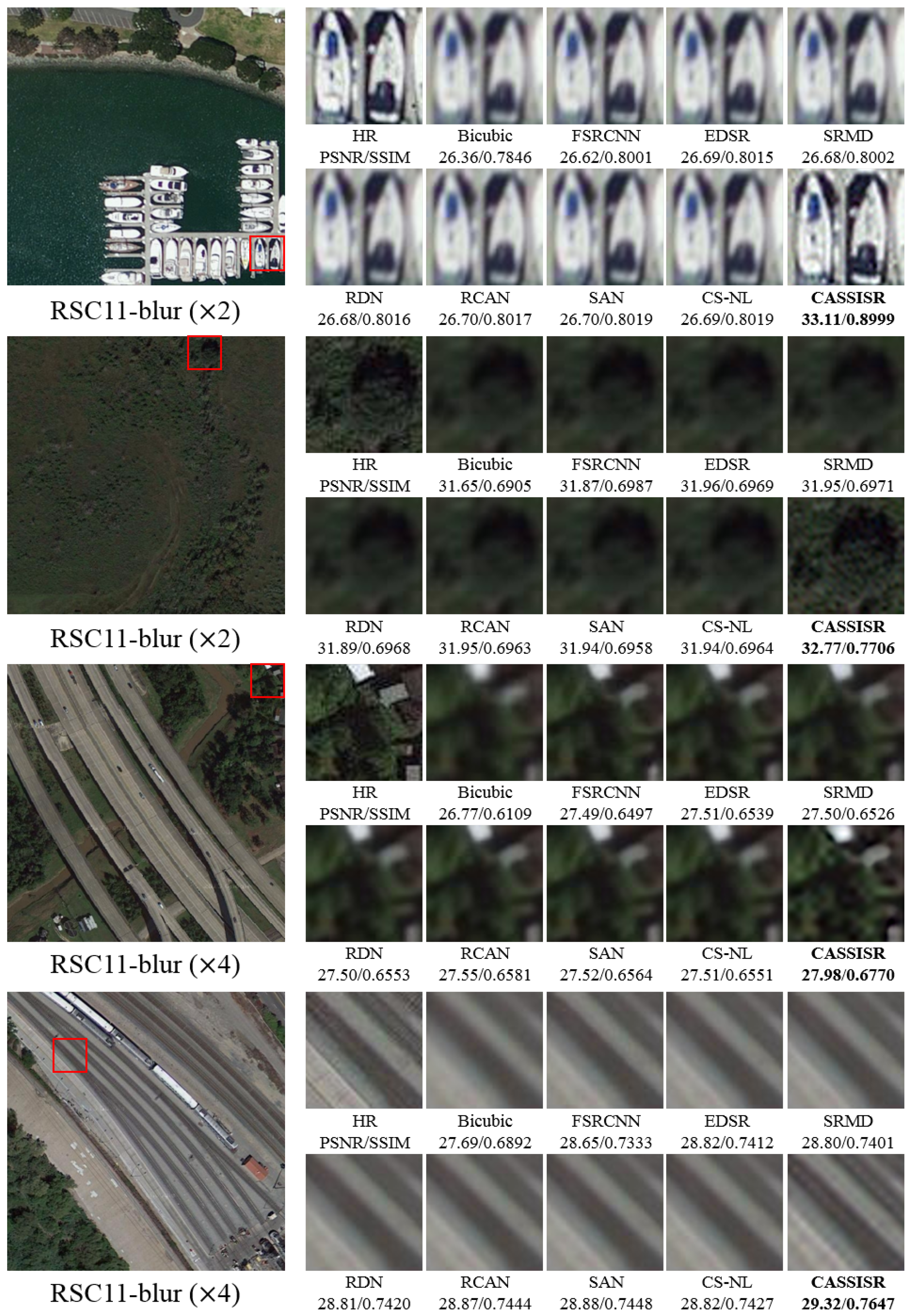
4.3.2. Qualitative Results

As shown in Figure 4, Figure 5, Figure 6, Figure 7, Figure 8 and Figure 9, we show the qualitative comparison results of scale factors $\times 2$ and $\times 4$ between CASSISR and CNN-based SR methods on RSSCN7-blur, RSC11-blur, WHU-RS19-blur, UC-Merced-blur, AID-blur, and NWPU45-blur datasets, respectively. It can be seen from the above visualization results that for the ‘non-ideal’ remote sensing dataset, the results of the CNN-based SR methods are fuzzy. In contrast, our CASSISR can recover more details and generate clearer HR images. Especially when the image has very strong internal repetitive features, the advantages of our CASSISR are more obvious. For example, the red house in Figure 4, the boat in Figure 5 and the car in Figure 6 can find many corresponding repetitive features from the image itself. It can be seen that for these images, our CASSISR improves more than the CNN-based SR methods.

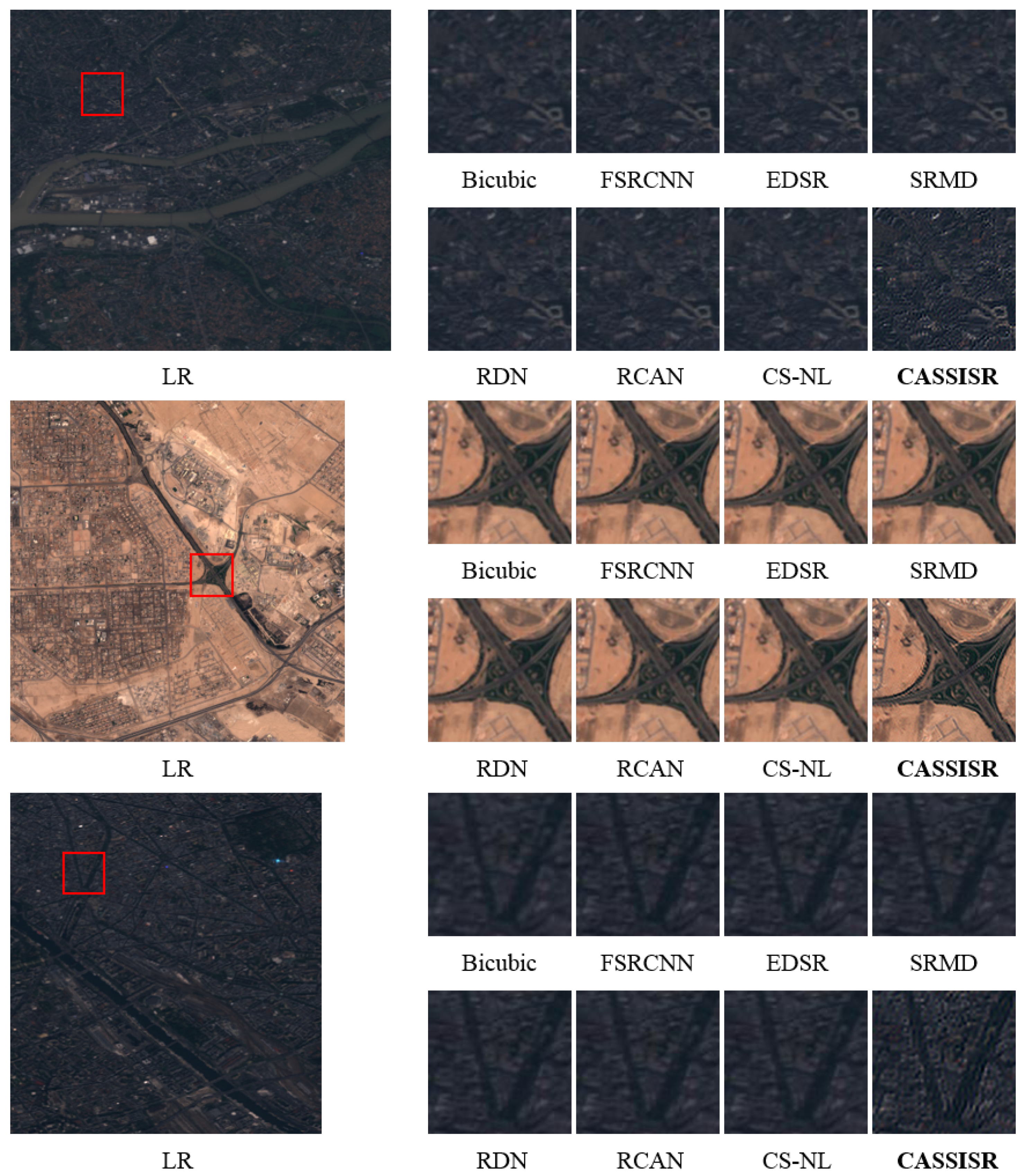
4.4. Experiments on the Real-World Remote Sensing Dataset

We evaluated our CASSISR on the real-world remote sensing dataset. We directly use the original image of OSCD [53] as input. Considering there is no ground truth as a control, we only show the result of the qualitative comparison. The qualitative comparison results of CASSISR and CNN-based SR methods in real-world remote sensing dataset are shown in Figure 10. The results generated by the CNN-based SR methods are low-quality. This is because the degradation process of real-world LR images is not simple bicubic downsampling. However, our CASSISR can make good use of the blur kernel estimated by KernelGAN [52] from the real image to generate a clearer image.

4.5. Ablation Experiment

We replaced our CDAM module with a CBAM [22] module and performed experiments on four datasets of RSSCN7, RSC11, RSSCN7-blur, and RSC11-blur, and performed a quantitative comparison with our CDAM. The experimental results are shown in

Table 3. Quantitative comparison of our CDAM and CBAM. Our CDAM results are highlighted, and the best results are underlined.

Method	Scale	RSSCN7	RSC11	RSSCN7-Blur	RSC11-Blur
		PSNR/SSIM	PSNR/SSIM	PSNR/SSIM	PSNR/SSIM
+CBAM [22]	$\times 2$	$32.87$/$0.8924$	$32.14$/$0.8826$	$29.87$/$0.8036$	$29.45$/$0.7952$
+CDAM(Our)	$\times 2$	$\underline{\mathbf{33}.\mathbf{01}}$/$\underline{\mathbf{0}.\mathbf{9027}}$	$\underline{\mathbf{32}.\mathbf{23}}$/$\underline{\mathbf{0}.\mathbf{8956}}$	$\underline{\mathbf{30}.\mathbf{01}}$/$\underline{\mathbf{0}.\mathbf{8142}}$	$\underline{\mathbf{29}.\mathbf{56}}$/$\underline{\mathbf{0}.\mathbf{8053}}$
+CBAM [22]	$\times 4$	$27.86$/$0.7058$	$27.03$/$0.6808$	$27.26$/$0.6848$	$26.33$/$0.6469$
+CDAM(Our)	$\times 4$	$\underline{\mathbf{27}.\mathbf{99}}$/$\underline{\mathbf{0}.\mathbf{7163}}$	$\underline{\mathbf{27}.\mathbf{13}}$/$\underline{\mathbf{0}.\mathbf{6913}}$	$\underline{\mathbf{27}.\mathbf{31}}$/$\underline{\mathbf{0}.\mathbf{6896}}$	$\underline{\mathbf{26}.\mathbf{44}}$/$\underline{\mathbf{0}.\mathbf{6613}}$

. On these four datasets, our CDAM is better than CBAM. Compared with CBAM, our CDAM infers effective 3-D weights by modeling the relationship between channel and spatial, which is more conducive to the learning of internal features of remote sensing images and improves the performance of remote sensing image SR.

5. Discussion

At present, most CNN-based SR methods and remote sensing SR methods usually assume that the image degradation process is bicubic downsampling, as shown in Equation (2). These methods use bicubic downsampling to construct a large number of training data pairs for long-term supervised training. However, the real image degradation process is complicated and is not simple bicubic downsampling. When these supervised SR methods are tested on real remote sensing images, their performance will drop significantly. Therefore, we need an SR algorithm that can process real-world remote sensing images.

In this study, we introduced the idea of self-supervised learning, took advantage of the cross-scale reproducibility of the powerful internal features of remote sensing images, and proposed the cross-dimension attention guided self-supervised remote sensing single-image super-resolution algorithm (CASSISR) that only requires one image for training. To better learn the internal characteristics of remote sensing images, we proposed a novel cross-dimension attention mechanism module (CDAM). Different from other attention models, we model the interdependence between the channel and the spatial features, jointly learn the feature weights of the channel and spatial, and consider the interaction between the channel dimension and the spatial dimension.

Through comparative experiments on three different types of datasets, our CASSISR outperforms other SOTA-SR methods in both a ‘non-ideal’ remote sensing dataset and real-world remote sensing dataset. On the ‘ideal’ remote sensing dataset, although our CASSISR was trained with only one image, it still achieved competitive results. This supervised network trained on a large number of datasets can produce better results when used on images that are also downsampled by the bicubic kernel, but this is not the focus of our research.

Our self-supervised method can better adapt to different Gaussian blur kernel downsampling and real-world LR remote sensing images. For the ‘non-ideal’ remote sensing dataset, our CASSISR obtains the best results under both $\times 2$ and $\times 4$ scale factors. It can be seen from Table 2 that both PSNR and SSIM have been significantly increased.

The PSNR: $+2.02$ dB and $+0.09$ dB for $\times 2$ and $\times 4$ scale on RSSCN7-blur, $+2.37$ dB and $+0.04$ dB for $\times 2$ and $\times 4$ scale on RSC11-blur, $+3.25$ dB and $+0.23$ dB for $\times 2$ and $\times 4$ scale on WHU-RS19-blur, $+3.52$ dB and $+0.12$ dB for $\times 2$ and $\times 4$ scale on UC-Merced-blur, $+2.95$ dB and $+0.27$ dB for $\times 2$ and $\times 4$ scale on AID-blur, $+2.63$ dB and $+0.11$ dB for $\times 2$ and $\times 4$ scale on NWPU45-blur.

The SSIM: $+0.0812$ and $+0.0034$ for $\times 2$ and $\times 4$ scale on RSSCN7-blur, $+0.0906$ and $+0.0012$ for $\times 2$ and $\times 4$ scale on RSC11-blur, $+0.0878$ and $+0.0072$ for $\times 2$ and $\times 4$ scale on WHU-RS19-blur, $+0.0936$ and $+0.0024$ for $\times 2$ and $\times 4$ scale on UC-Merced-blur, $+0.0749$ and $+0.0020$ for $\times 2$ and $\times 4$ scale on AID-blur, $+0.0941$ and $+0.0007$ for $\times 2$ and $\times 4$ scale on NWPU45-blur.

It can also be seen from the visualization results in Figure 4, Figure 5, Figure 6, Figure 7, Figure 8 and Figure 9 that the HR images generated by our CASSISR are clearer. For real-world remote sensing images, our CASSISR can still generate better results than other CNN-based SR methods. As can be seen from Figure 10, the result generated by our CASSISR has more details and textures, while the image generated by the CNN-based SR methods is blurred. The results show that the CNN-based SR methods trained with an ‘ideal’ dataset are effective in processing bicubic downsampled images, but the ability to process unknown Gaussian blur kernel downsampling and real-world LR remote sensing images is insufficient. However, our CASSISR uses a self-supervised method to learn inter-scale repetitive features within remote sensing images for SR of remote sensing images. In ‘non-ideal’ and real-world situations, the performance of CASSISR trained on only one image is better than the SOTA-SR methods trained on large datasets.

6. Conclusions

In this paper, we propose a cross-dimension attention guided self-supervised remote sensing single-image super-resolution method (CASSISR), which does not require datasets for prior training. Only one image is needed to train the cross-dimension attention network (CDAN). The proposed cross-dimension attention mechanism module (CDAM) models the interdependence between the channel and spatial feature and jointly learns the feature weights of the channel and spatial to better capture the global features inside the image. Experiments have proved that CASSISR can better adapt to real remote sensing image SR tasks. Using only one image to train the SR model can save a lot of computing resources, which provides a new idea for the SR of remote sensing images.

References

1. Minh-Tan, P.; Aptoula, E.; Lefèvre, S. Feature profiles from attribute filtering for classification of remote sensing images. IEEE J. Sel. Top. Appl. Earth Observ. Remote Sens. 2017, 11, 249–256. [Google Scholar]
2. Maxwell, A.E.; Warner, T.A.; Fang, F. Implementation of machine-learning classification in remote sensing: An applied review. Int. J. Remote Sens. 2018, 39, 2784–2817. [Google Scholar] [CrossRef] [Green Version]
3. Gencer, S.; Cinbis, R.G.; Aksoy, S. Fine-grained object recognition and zero-shot learning in remote sensing imagery. IEEE Trans. Geosci. Remote Sens. 2017, 56, 770–779. [Google Scholar]
4. Kong, X.; Huang, Y.; Li, S.; Lin, H.; Benediktsson, J.A. Extended random walker for shadow detection in very high resolution remote sensing images. IEEE Trans. Geosci. Remote Sens. 2017, 56, 867–876. [Google Scholar] [CrossRef]
5. Lin, H.; Shi, Z.; Zou, Z. Fully convolutional network with task partitioning for inshore ship detection in optical remote sensing images. IEEE Geosci. Remote Sens. Lett. 2017, 14, 1665–1669. [Google Scholar] [CrossRef]
6. Wu, T.; Luo, J.; Fang, J.; Ma, J.; Song, X. Unsupervised object-based change detection via a Weibull mixture model-based binarization for high-resolution remote sensing images. IEEE Geosci. Remote Sens. Lett. 2017, 15, 63–67. [Google Scholar] [CrossRef]
7. Liu, Z.; Li, G.; Mercier, G.; He, Y.; Pan, Q. Change detection in heterogenous remote sensing images via homogeneous pixel transformation. IEEE Trans. Image Process. 2017, 27, 1822–1834. [Google Scholar] [CrossRef]
8. Zhang, L.; Wu, X. An edge-guided image interpolation algorithm via directional filtering and data fusion. IEEE Trans. Image Process. 2006, 15, 2226–2238. [Google Scholar] [CrossRef] [Green Version]
9. Zhang, K.; Gao, X.; Tao, D.; Li, X. Single image super-resolution with non-local means and steering kernel regression. IEEE Trans. Image Process. 2012, 21, 4544–4556. [Google Scholar] [CrossRef]
10. Dong, C.; Loy, C.C.; He, K.; Tang, X. Learning a deep convolutional network for image super-resolution. In Proceedings of the European Conference on Computer Vision, Zurich, Switzerland, 6–12 September 2014; pp. 184–199. [Google Scholar]
11. Kim, J.; Lee, J.K.; Lee, K.M. Accurate image super-resolution using very deep convolutional networks. In Proceedings of the IEEE Conference on Computer Vision and Pattern Recognition, Las Vegas, NV, USA, 26 June–1 July 2016; pp. 1646–1654. [Google Scholar]
12. Zhang, K.; Zuo, W.; Zhang, L. Learning a single convolutional super-resolution network for multiple degradations. In Proceedings of the IEEE Conference on Computer Vision and Pattern Recognition, Salt Lake City, UT, USA, 18–23 June 2018; pp. 3262–3271. [Google Scholar]
13. Dai, T.; Cai, J.; Zhang, Y.; Xia, S.T.; Zhang, L. Second-order attention network for single image super-resolution. In Proceedings of the IEEE Conference on Computer Vision and Pattern Recognition, Long Beach, CA, USA, 16–20 June 2019; pp. 11065–11074. [Google Scholar]
14. Haris, M.; Shakhnarovich, G.; Ukita, N. Deep back-projection networks for super-resolution. In Proceedings of the IEEE Conference on Computer Vision and Pattern Recognition, Salt Lake City, UT, USA, 18–23 June 2018; pp. 1664–1673. [Google Scholar]
15. Zhang, Y.; Tian, Y.; Kong, Y.; Zhong, B.; Fu, Y. Residual dense network for image super-resolution. In Proceedings of the IEEE Conference on Computer Vision and Pattern Recognition, Salt Lake City, UT, USA, 18–23 June 2018; pp. 2472–2481. [Google Scholar]
16. He, K.; Zhang, X.; Ren, S.; Sun, J. Deep residual learning for image recognition. In Proceedings of the IEEE Conference on Computer Vision and Pattern Recognition, Las Vegas, NV, USA, 26 June–1 July 2016; pp. 770–778. [Google Scholar]
17. Kim, J.; Lee, J.K.; Lee, K.M. Deeply-recursive convolutional network for image super-resolution. In Proceedings of the IEEE Conference on Computer Vision and Pattern Recognition, Las Vegas, NV, USA, 26 June–1 July 2016; pp. 1637–1645. [Google Scholar]
18. Lim, B.; Son, S.; Kim, H.; Nah, S.; Lee, K.M. Enhanced deep residual networks for single image super-resolution. In Proceedings of the IEEE Conference on Computer Vision and Pattern Recognition, Honolulu, HI, USA, 21–26 July 2017; pp. 136–144. [Google Scholar]
19. Tai, Y.; Yang, J.; Liu, X. Image super-resolution via deep recursive residual network. In Proceedings of the IEEE Conference on Computer Vision and Pattern Recognition, Honolulu, HI, USA, 21–26 July 2017; pp. 3147–3155. [Google Scholar]
20. Sajjadi, M.S.; Scholkopf, B.; Hirsch, M. Enhancenet: Single image super-resolution through automated texture synthesis. In Proceedings of the 2017 IEEE International Conference on Computer Vision, Venice, Italy, 22–29 October 2017; pp. 4491–4500. [Google Scholar]
21. Hu, J.; Shen, L.; Sun, G. Squeeze-and-excitation networks. In Proceedings of the IEEE Conference on Computer Vision and Pattern Recognition, Salt Lake City, UT, USA, 18–23 June 2018; pp. 7132–7141. [Google Scholar]
22. Woo, S.; Park, J.; Lee, J.Y.; Kweon, I.S. Cbam: Convolutional block attention module. In Proceedings of the European Conference on Computer Vision, Munich, Germany, 8–14 September 2018; pp. 3–19. [Google Scholar]
23. Zhang, Y.; Li, K.; Li, K.; Wang, L.; Zhong, B.; Fu, Y. Image super-resolution using very deep residual channel attention networks. In Proceedings of the European Conference on Computer Vision, Munich, Germany, 8–14 September 2018; pp. 286–301. [Google Scholar]
24. Hu, Y.; Li, J.; Huang, Y.; Gao, X. Channel-wise and spatial feature modulation network for single image super-resolution. IEEE Trans. Circuits Syst. Video Technol. 2019, 30, 3911–3927. [Google Scholar] [CrossRef] [Green Version]
25. Agustsson, E.; Timofte, R. Ntire 2017 challenge on single image super-resolution: Dataset and study. In Proceedings of the IEEE Conference on Computer Vision and Pattern Recognition, Honolulu, HI, USA, 21–26 July 2017; pp. 126–135. [Google Scholar]
26. Glasner, D.; Bagon, S.; Irani, M. Super-resolution from a single image. In Proceedings of the IEEE International Conference on Computer Vision, Kyoto, Japan, 29 September–2 October 2009; pp. 349–356. [Google Scholar]
27. Huang, J.B.; Singh, A.; Ahuja, N. Single image super-resolution from transformed self-exemplars. In Proceedings of the IEEE Conference on Computer Vision and Pattern Recognition, Boston, MA, USA, 7–12 June 2015; pp. 5197–5206. [Google Scholar]
28. Michaeli, T.; Irani, M. Nonparametric blind super-resolution. In Proceedings of the 2013 IEEE International Conference on Computer Vision, Sydney, Australia, 1–8 December 2013; pp. 945–952. [Google Scholar]
29. Bahat, Y.; Efrat, N.; Irani, M. Non-uniform blind deblurring by reblurring. In Proceedings of the 2017 IEEE International Conference on Computer Vision, Venice, Italy, 22–29 October 2017; pp. 3286–3294. [Google Scholar]
30. Bahat, Y.; Irani, M. Blind dehazing using internal patch recurrence. In Proceedings of the IEEE International Conference on Computer Photography, Evanston, IL, USA, 13–15 May 2016; pp. 1–9. [Google Scholar]
31. Shocher, A.; Cohen, N.; Irani, M. “zero-shot” super-resolution using deep internal learning. In Proceedings of the IEEE Conference on Computer Vision and Pattern Recognition, Salt Lake City, UT, USA, 18–23 June 2018; pp. 3118–3126. [Google Scholar]
32. Xu, X.; Sun, D.; Pan, J.; Zhang, Y.; Pfister, H.; Yang, M.H. Learning to super-resolve blurry face and text images. In Proceedings of the 2017 IEEE International Conference on Computer Vision, Venice, Italy, 22–29 October 2017; pp. 251–260. [Google Scholar]
33. Zhang, X.; Chen, Q.; Ng, R.; Koltun, V. Zoom to learn, learn to zoom. In Proceedings of the IEEE Conference on Computer Vision and Pattern Recognition, Long Beach, CA, USA, 16–20 June 2019; pp. 3762–3770. [Google Scholar]
34. Zontak, M.; Irani, M. Internal statistics of a single natural image. In Proceedings of the IEEE Conference on Computer Vision and Pattern Recognition, Providence, RI, USA, 20–25 June 2011; pp. 977–984. [Google Scholar]
35. Dong, C.; Loy, C.C.; Tang, X. Accelerating the super-resolution convolutional neural network. In Proceedings of the European Conference on Computer Vision, Amsterdam, The Netherlands, 8–16 October 2016; pp. 391–407. [Google Scholar]
36. Huang, N.; Yang, Y.; Liu, J.; Gu, X.; Cai, H. Single-image super-resolution for remote sensing data using deep residual-learning neural network. In Proceedings of the Springer International Conference on Neural Information Processing, Guangzhou, China, 14–18 November 2017; pp. 622–630. [Google Scholar]
37. Lei, S.; Shi, Z.; Zou, Z. Super-Resolution for Remote Sensing Images via Local–Global Combined Network. IEEE Geosci. Remote Sens. Lett. 2017, 14, 1243–1247. [Google Scholar] [CrossRef]
38. Xu, W.; Xu, G.; Wang, Y.; Sun, X.; Lin, D.; Wu, Y. Deep memory connected neural network for optical remote sensing image restoration. Remote Sens. 2018, 10, 1893. [Google Scholar] [CrossRef] [Green Version]
39. Gu, J.; Sun, X.; Zhang, Y.; Fu, K.; Wang, L. Deep Residual Squeeze and Excitation Network for Remote Sensing Image Super-Resolution. Remote Sens. 2019, 11, 1817. [Google Scholar] [CrossRef] [Green Version]
40. Haut, J.M.; Paoletti, M.E.; Fernandez-Beltran, R.; Plaza, J.; Plaza, A.; Li, J. Remote Sensing Single-Image Superresolution Based on a Deep Compendium Model. IEEE Geosci. Remote Sens. Lett. 2019, 16, 1432–1436. [Google Scholar] [CrossRef]
41. Jaderberg, M.; Simonyan, K.; Zisserman, A.; Kavukcuoglu, K. Spatial transformer networks. In Proceedings of the Advances in Neural Information Processing Systems 28, Montreal, QC, Canada, 7–12 December 2015; pp. 2017–2025. [Google Scholar]
42. Gao, Z.; Xie, J.; Wang, Q.; Li, P. Global second-order pooling convolutional networks. In Proceedings of the IEEE Conference on Computer Vision and Pattern Recognition, Long Beach, CA, USA, 16–20 June 2019; pp. 3024–3033. [Google Scholar]
43. Hu, J.; Shen, L.; Albanie, S.; Sun, G.; Vedaldi, A. Gather-excite: Exploiting feature context in convolutional neural networks. In Proceedings of the NIPS 2018: The 32nd Annual Conference on Neural Information Processing Systems, Montreal, QC, Canada, 3–8 December 2018; pp. 1–11. [Google Scholar]
44. Park, J.; Woo, S.; Lee, J.Y.; Kweon, I.S. BAM: Bottleneck Attention Module. In Proceedings of the 2018 British Machine Vision Conference, Newcastle, UK, 3–6 September 2018; pp. 147–163. [Google Scholar]
45. Kingma, D.P.; Ba, J. Adam: A method for stochastic optimization. arXiv 2018, arXiv:1412.6980. [Google Scholar]
46. Zou, Q.; Ni, L.; Zhang, T.; Wang, Q. Deep learning based feature selection for remote sensing scene classification. IEEE Geosci. Remote Sens. Lett. 2015, 12, 2321–2325. [Google Scholar] [CrossRef]
47. Zhao, L.; Tang, P.; Huo, L. Feature significance-based multibag-of-visual-words model for remote sensing image scene classification. J. Appl. Remote Sens. 2016, 10, 035004. [Google Scholar] [CrossRef]
48. Sheng, G.; Yang, W.; Xu, T.; Sun, H. High-resolution satellite scene classification using a sparse coding based multiple feature combination. Int. J. Remote Sens. 2012, 33, 2395–2412. [Google Scholar] [CrossRef]
49. Yang, Y.; Newsam, S. Bag-of-visual-words and spatial extensions for land-use classification. In Proceedings of the 18th SIGSPATIAL International Conference on Advances in Geographic Information Systems, San Jose, CA, USA, 2–5 November 2010; pp. 270–279. [Google Scholar]
50. Xia, G.S.; Hu, J.; Hu, F.; Shi, B.; Bai, X.; Zhong, Y.; Zhang, L. AID: A benchmark data set for performance evaluation of aerial scene classification. IEEE Trans. Geosci. Remote Sens. 2017, 55, 3965–3981. [Google Scholar] [CrossRef] [Green Version]
51. Cheng, G.; Han, J.; Lu, X. Remote sensing image scene classification: Benchmark and state of the art. Proc. IEEE 2017, 105, 1865–1883. [Google Scholar] [CrossRef] [Green Version]
52. Bell-Kligler, S.; Shocher, A.; Irani, M. Blind super-resolution kernel estimation using an internal-gan. In Proceedings of the Advances in Neural Information Processing Systems, Vancouver, BC, Canada, 8–14 December 2019; pp. 284–293. [Google Scholar]
53. Daudt, R.C.; Saux, B.L.; Boulch, A.; Gousseau, Y. Urban change detection for multispectral earth observation using convolutional neural networks. In Proceedings of the IEEE International Geoscience and Remote Sensing Symposium, Valencia, Spain, 22–27 July 2018; pp. 2115–2118. [Google Scholar]
54. Mei, Y.; Fan, Y.; Zhou, Y.; Huang, L.; Huang, T.S.; Shi, H. Image Super-Resolution With Cross-Scale Non-Local Attention and Exhaustive Self-Exemplars Mining. In Proceedings of the IEEE Conference on Computer Vision and Pattern Recognition, Seattle, WA, USA, 14–19 June 2020; pp. 5690–5699. [Google Scholar]
55. Wang, X.; Wu, Y.; Ming, Y.; Lv, H. Remote Sensing Imagery Super Resolution Based on Adaptive Multi-Scale Feature Fusion Network. Remote Sens. 2020, 20, 1142. [Google Scholar] [CrossRef] [Green Version]
Figure 1. Cross-scale internal information reproducibility of remote sensing images. The information inside the same picture (small-scale information in the red frame) can be found in other places (large-scale information in the blue frame) for the existence of different scales.
Remotesensing 13 03835 g001
Figure 2. The overall structure of cross-dimension attention guided self-supervised remote sensing single-image super-resolution (CASSISR). Among them, CDAM is the proposed cross-dimension attention module.
Remotesensing 13 03835 g002
Figure 3. The structure of the cross-dimension attention module. C × H × W denotes a feature map with the number of channels C , the height of H and the width of W . ⊗ denotes matrix multiplication. ⊙ denotes element-wise multiplication.
Remotesensing 13 03835 g003
Figure 4. Qualitative comparison of scaling factors × 2 and × 4 between CASSISR and CNN-based SR methods on RSSCN7-blur dataset. Our CASSISR results are highlighted.
Remotesensing 13 03835 g004
Figure 5. Qualitative comparison of scaling factors × 2 and × 4 between CASSISR and CNN-based SR methods on RSC11-blur dataset. Our CASSISR results are highlighted.
Remotesensing 13 03835 g005
Figure 6. Qualitative comparison of scaling factors × 2 and × 4 between CASSISR and CNN-based SR methods on WHU-RS19-blur dataset. Our CASSISR results are highlighted.
Remotesensing 13 03835 g006
Figure 7. Qualitative comparison of scaling factors × 2 and × 4 between CASSISR and CNN-based SR methods on UC-Merced-blur dataset. Our CASSISR results are highlighted.
Remotesensing 13 03835 g007
Figure 8. Qualitative comparison of scaling factors × 2 and × 4 between CASSISR and CNN-based SR methods on AID-blur dataset. Our CASSISR results are highlighted.
Remotesensing 13 03835 g008
Figure 9. Qualitative comparison of scaling factors × 2 and × 4 between CASSISR and CNN-based SR methods on NWPU45-blur dataset. Our CASSISR results are highlighted.
Remotesensing 13 03835 g009
Figure 10. Qualitative comparison between CASSISR and CNN-based SR methods on real-world remote sensing dataset.
Remotesensing 13 03835 g010