
Integrating Multi-Sensors Data for Species Distribution Mapping Using Deep Learning and Envelope Models

 , ,
, ,  , and
, and
Abstract
:
1. Introduction
2. Materials and Methods
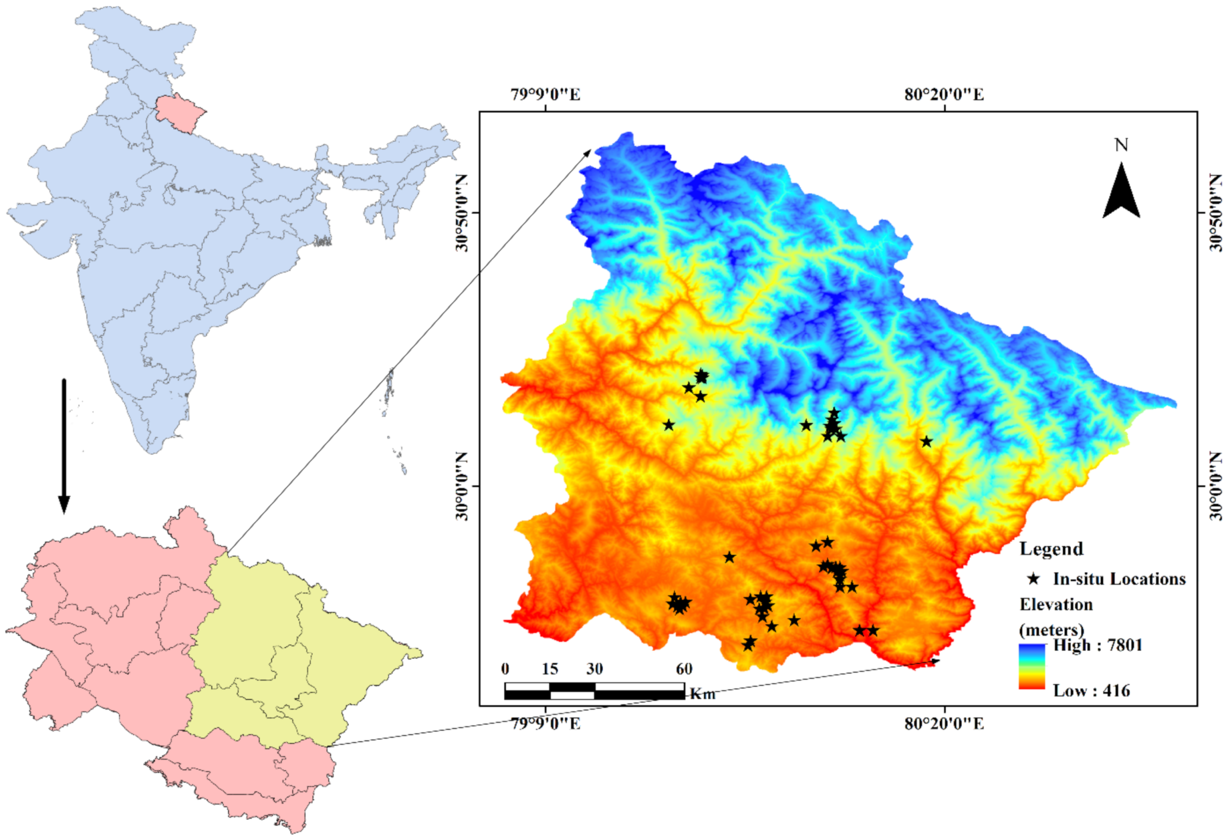
2.1. Study Area
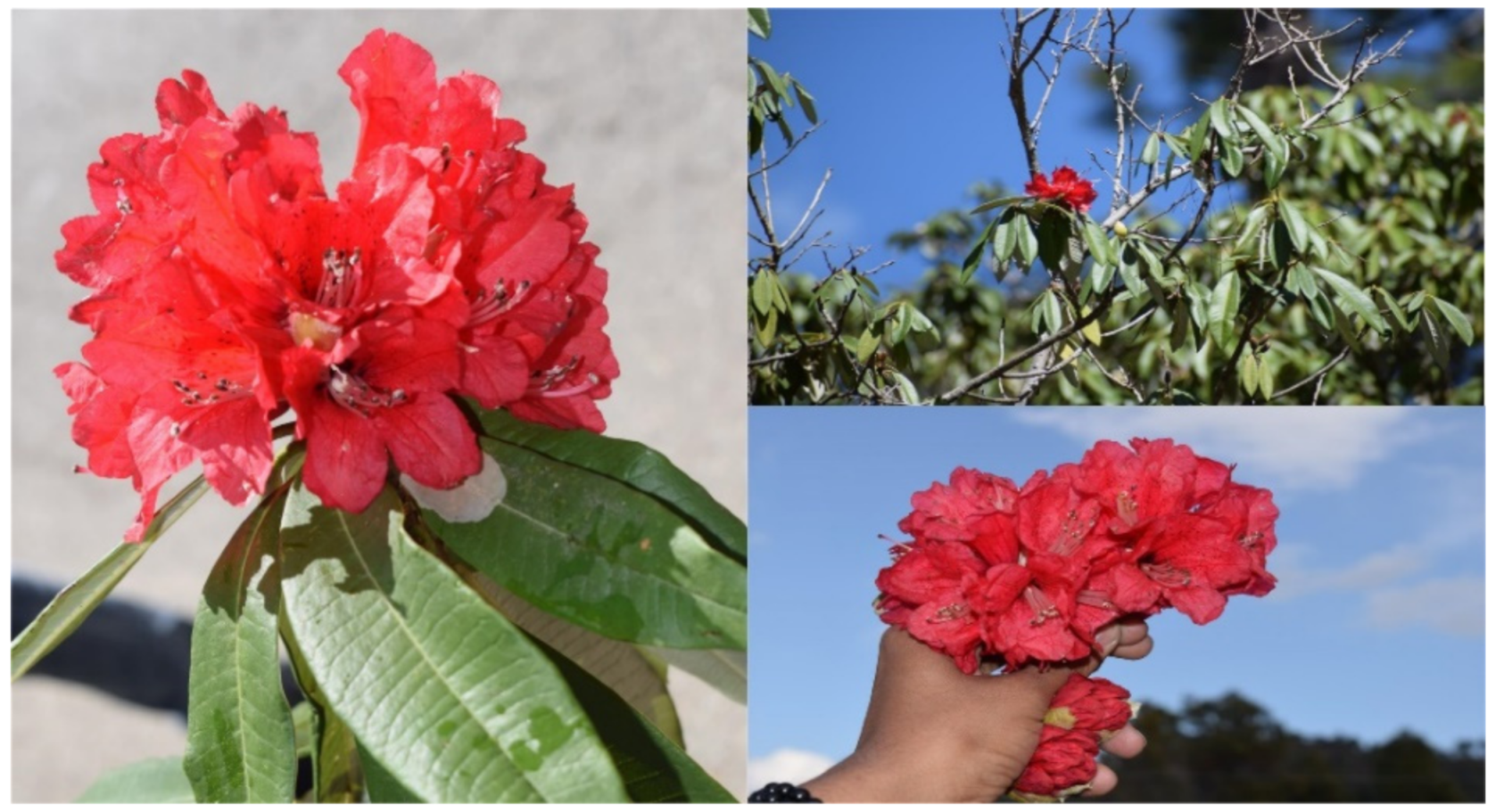
2.2. Target Species and Occurrence Data
2.3. Environmental Variables
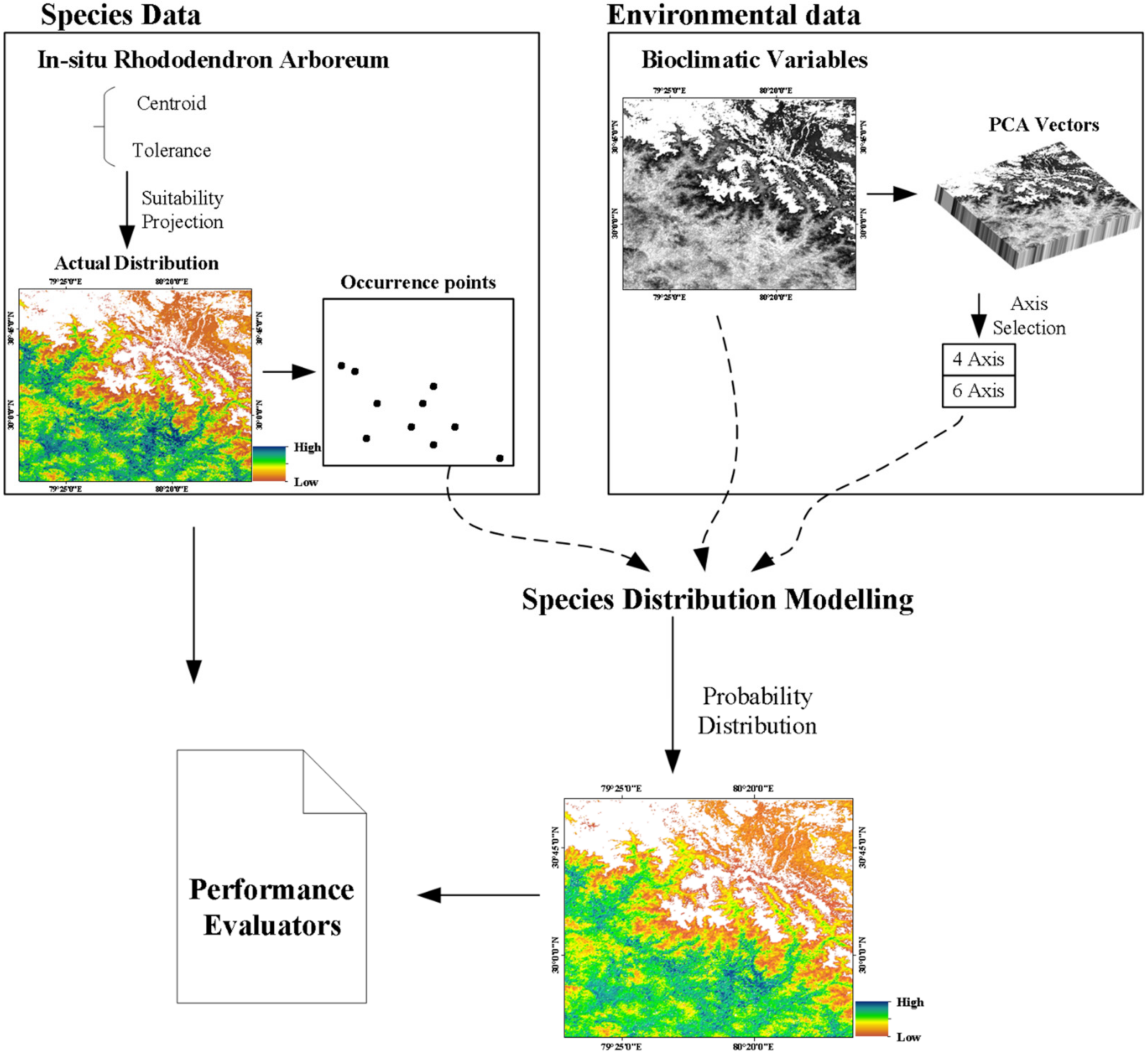
2.4. Ecological Niche Modelling
2.4.1. BIOCLIM
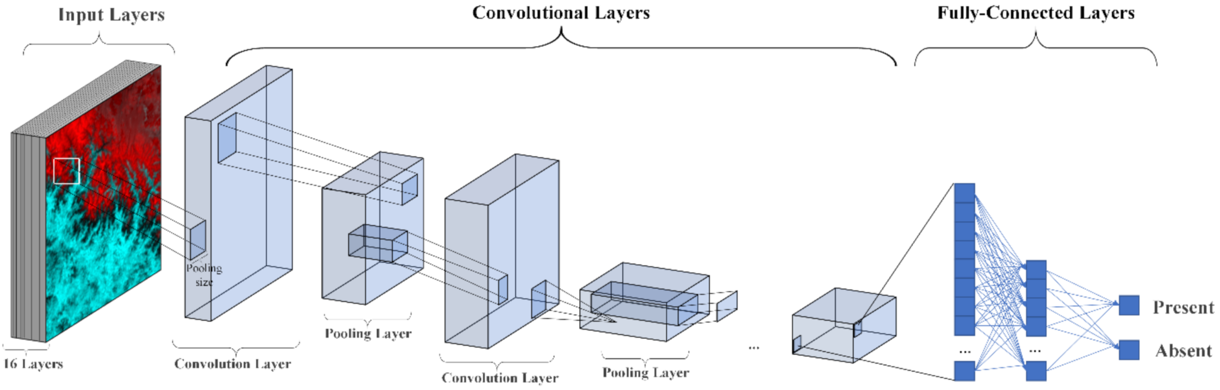
2.4.2. CNN
2.5. Model Validation
3. Results
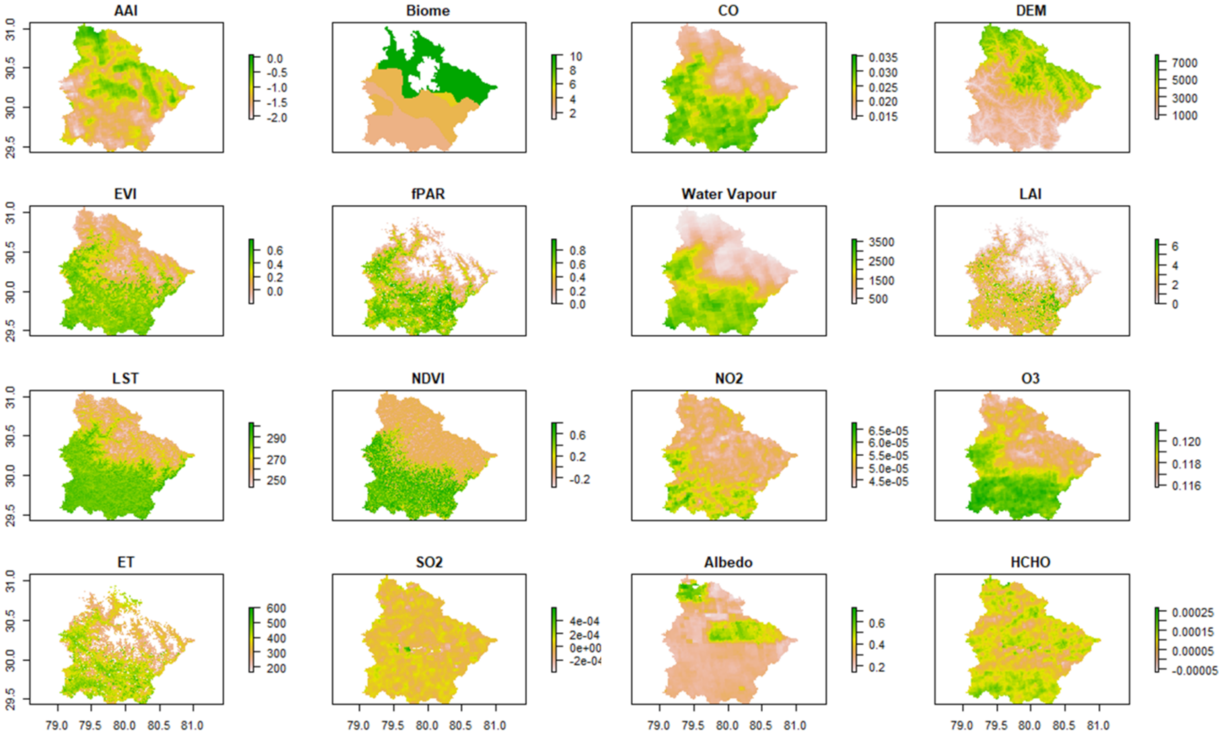
3.1. Assessing the Distribution of Input Parameters
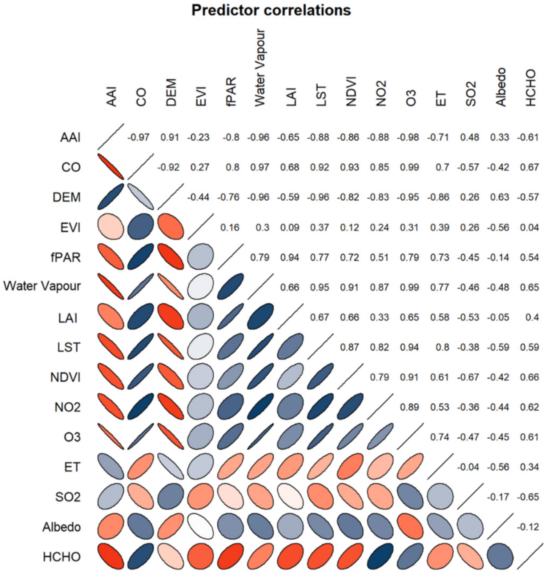
3.2. Understanding Parameter Intercorrelation
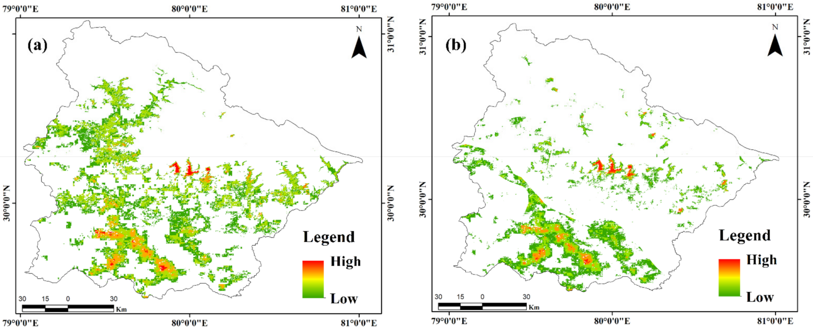
3.3. Spatial Distribution of Rhododendron arboreum
3.4. Model Validation and Comparison
4. Discussion
5. Conclusions
Supplementary Materials
Author Contributions
Funding
Institutional Review Board Statement
Informed Consent Statement
Data Availability Statement
Acknowledgments
Conflicts of Interest
References
- Sabin, T.; Krishnan, R.; Vellore, R.; Priya, P.; Borgaonkar, H.; Singh, B.B.; Sagar, A. Climate change over the Himalayas. In Assessment of Climate Change over the Indian Region; Krishnan, R., Sanjay, J., Gnanaseelan, C., Mujumdar, M., Kulkarni, A., Chakraborty, S., Eds.; Springer: Singapore, 2020; pp. 207–222. [Google Scholar]
- Kraaijenbrink, P.D.; Bierkens, M.; Lutz, A.; Immerzeel, W. Impact of a global temperature rise of 1.5 degrees Celsius on Asia’s glaciers. Nature 2017, 549, 257–260. [Google Scholar] [CrossRef]
- Kala, C.P. Status and conservation of rare and endangered medicinal plants in the Indian trans-Himalaya. Biol. Conserv. 2000, 93, 371–379. [Google Scholar] [CrossRef]
- Veera, S.N.; Panda, R.M.; Behera, M.D.; Goel, S.; Roy, P.S.; Barik, S.K. Prediction of upslope movement of Rhododendron arboreum in Western Himalaya. Trop. Ecol. 2019, 60, 518–524. [Google Scholar] [CrossRef]
- Srivastava, P. Rhododendron arboreum: An overview. J. Appl. Pharm. Sci. 2012, 2, 158–162. [Google Scholar]
- Bhandari, M.S.; Meena, R.K.; Shankhwar, R.; Shekhar, C.; Saxena, J.; Kant, R.; Pandey, V.V.; Barthwal, S.; Pandey, S.; Chandra, G. Prediction mapping through maxent modeling paves the way for the conservation of Rhododendron arboreum in Uttarakhand Himalayas. J. Indian Soc. Remote Sens. 2020, 48, 411–422. [Google Scholar] [CrossRef]
- Jain, A.; Pandit, M.K.; Elahi, S.; Jain, A.; Bhaskar, A.; Kumar, V. Reproductive behaviour and genetic variability in geographically isolated populations of Rhododendron arboreum (Ericaceae). Curr. Sci. 2000, 79, 1377–1381. [Google Scholar]
- Sharma, G. Development and Charaterization of UGMS Markers for Genetic Diversity Analysis in Rhododendron Arboreum; Guru Kashi University: Punjab, India, 2013. [Google Scholar]
- Chauhan, D.; Lal, P.; Singh, D. Composition, population structure and regeneration of Rhododendron arboreum Sm. temperate broad-leaved evergreen forest in Garhwal Himalaya, Uttarakhand, India. J. Earth Sci. Clim. Chang. 2017, 8, 430. [Google Scholar] [CrossRef]
- Humboldt, A.V.; Bonpland, A. Ideen Zu Einer Geographie Der Pflanzen Nebst Einem Naturgemälde Der Tropenländer; Cotta: Tübingen, Germany, 1807. [Google Scholar]
- De Candolle, A. Géographie Botanique Raisonnée Ou Exposition Des Faits Principaux Et Des Lois Concernant La Distribution Géographique Des Plantes De L’époque Actuelle; V. Masson: Paris, France, 1855; Volume 2. [Google Scholar]
- Udvardy, M.F. Notes on the ecological concepts of habitat, biotope and niche. Ecology 1959, 40, 725–728. [Google Scholar] [CrossRef]
- Priti, H.; Aravind, N.; Shaanker, R.U.; Ravikanth, G. Modeling impacts of future climate on the distribution of Myristicaceae species in the Western Ghats, India. Ecol. Eng. 2016, 89, 14–23. [Google Scholar] [CrossRef]
- Adhikari, D.; Barik, S.; Upadhaya, K. Habitat distribution modelling for reintroduction of Ilex khasiana Purk., a critically endangered tree species of northeastern India. Ecol. Eng. 2012, 40, 37–43. [Google Scholar] [CrossRef] [Green Version]
- Franklin, J. Moving beyond static species distribution models in support of conservation biogeography. Divers. Distrib. 2010, 16, 321–330. [Google Scholar] [CrossRef]
- Vasconcelos, T.S.; Rodríguez, M.Á.; Hawkins, B.A. Species distribution modelling as a macroecological tool: A case study using New World amphibians. Ecography 2012, 35, 539–548. [Google Scholar] [CrossRef]
- Rodríguez, J.P.; Brotons, L.; Bustamante, J.; Seoane, J. The application of predictive modelling of species distribution to biodiversity conservation. Divers. Distrib. 2007, 13, 243–251. [Google Scholar] [CrossRef]
- Lorena, A.C.; Jacintho, L.F.; Siqueira, M.F.; De Giovanni, R.; Lohmann, L.G.; De Carvalho, A.C.; Yamamoto, M. Comparing machine learning classifiers in potential distribution modelling. Expert Syst. Appl. 2011, 38, 5268–5275. [Google Scholar] [CrossRef]
- Elith, J.; Leathwick, J.R. Species distribution models: Ecological explanation and prediction across space and time. Annu. Rev. of Ecol. Evol. Syst. 2009, 40, 677–697. [Google Scholar] [CrossRef]
- Rana, S.K.; Rana, H.K.; Luo, D.; Sun, H. Estimating climate-induced ‘Nowhere to go’range shifts of the Himalayan Incarvillea Juss. using multi-model median ensemble species distribution models. Ecol. Indic. 2021, 121, 107127. [Google Scholar] [CrossRef]
- Beaumont, L.J.; Hughes, L.; Poulsen, M. Predicting species distributions: Use of climatic parameters in BIOCLIM and its impact on predictions of species’ current and future distributions. Ecol. Model. 2005, 186, 251–270. [Google Scholar] [CrossRef]
- Doran, B.; Olsen, P. Customizing BIOCLIM to investigate spatial and temporal variations in highly mobile species. In Proceedings of the 6th International Conference in GeoComputation, Brisbane, Australia, 24–26 September 2001. [Google Scholar]
- Xu, Y.; Zhou, P.-Y.; Wang, Y.; Chen, Z.-X.; Ma, R.; Yu, S.-F. Assessment of risk of introduction of pine wood nematode, bursaphelenchus xylophilus in Yunnan Province using BIOCLIM ecological niche model. J. Yunnan Agric. Univ. 2008, 23, 746–753. [Google Scholar]
- Bhatta, K.P.; Robson, B.A.; Suwal, M.K.; Vetaas, O.R. A pan-Himalayan test of predictions on plant species richness based on primary production and water-energy dynamics. Front. Biogeogr. 2021, 13, e49459. [Google Scholar]
- Mamgain, A.; Uniyal, P.L. Species Distribution Modelling of Rhododendron arboreum Sm.–A Keystone Species, in India and Adjoining Region. Int. J. Ecol. Environ. Sci. 2018, 44, 261–286. [Google Scholar]
- Goodfellow, I.; Bengio, Y.; Courville, A. Deep Learning; MIT press: Cambridge, MA, USA, 2016. [Google Scholar]
- Lek, S.; Delacoste, M.; Baran, P.; Dimopoulos, I.; Lauga, J.; Aulagnier, S. Application of neural networks to modelling nonlinear relationships in ecology. Ecol. Model. 1996, 90, 39–52. [Google Scholar] [CrossRef]
- Thuiller, W. BIOMOD–optimizing predictions of species distributions and projecting potential future shifts under global change. Glob. Chang. Biol. 2003, 9, 1353–1362. [Google Scholar] [CrossRef]
- Zhang, J.; Li, S. A Review of Machine Learning Based Species’ Distribution Modelling. In Proceedings of the 2017 International Conference on Industrial Informatics-Computing Technology, Intelligent Technology, Industrial Information Integration (ICIICII), Wuhan, China, 2–3 December 2017; pp. 199–206. [Google Scholar]
- Kumar, K. Water Management in Himalayan Ecosystem: A Study of Natural Springs of Almora; Indus Publishing: New Delhi, India, 1996. [Google Scholar]
- Phillips, S.J.; Anderson, R.P.; Schapire, R.E. Maximum entropy modeling of species geographic distributions. Ecol. Model. 2006, 190, 231–259. [Google Scholar] [CrossRef] [Green Version]
- Tewari, A.P. Recent changes in the position of the snout of the Pindari glacier (Kumaon Himalaya), Almora District, Uttar Pradesh, India. In Proceedings of the Role of Snow and Ice in Hydrology, Banff Symposia, September 1972; WMO-IAHS-Unesco: Geneva, Switzerland, 1973; pp. 1144–1149. [Google Scholar]
- Singh, K.; Rai, L.; Gurung, B. Conservation of rhododendrons in Sikkim Himalaya: An overview. World J. Agric. Sci. 2009, 5, 284–296. [Google Scholar]
- Secretariat, G. GBIF backbone taxonomy. Checklist Dataset 2017, 10. Available online: https://www.gbif.org/dataset/d7dddbf4-2cf0-4f39-9b2a-bb099caae36c (accessed on 5 June 2021).
- Rawat, P.; Rai, N.; Kumar, N.; Bachheti, R. Review on Rhododendron arboreum—A magical tree. Orient. Pharm. Exp. Med. 2017, 17, 297–308. [Google Scholar] [CrossRef]
- Paul, A.; Khan, M.L.; Arunachalam, A.; Arunachalam, K. Biodiversity and conservation of rhododendrons in Arunachal Pradesh in the Indo-Burma biodiversity hotspot. Curr. Sci. 2005, 89, 623–634. [Google Scholar]
- Chauhan, N.S. Medicinal and Aromatic Plants of Himachal Pradesh; Indus Publishing: New Delhi, India, 1999. [Google Scholar]
- Watts, J.S. When a Billion Chinese Jump: How China Will Save Mankind—Or Destroy It; Simon and Schuster: New York, NY, USA, 2010. [Google Scholar]
- Singh, V.K.; Ali, Z.A. Herbal Drugs of Himalaya; Today & Tomorrow’s Printers and Publishers: Delhi, India, 1998. [Google Scholar]
- Singh, N.; Ram, J.; Tewari, A.; Yadav, R. Phenological events along the elevation gradient and effect of climate change on Rhododendron arboreum Sm. in Kumaun Himalaya. Curr. Sci. 2015, 108, 106–110. [Google Scholar]
- Paul, A.; Khan, M.L.; Das, A.K. Utilization of Rhododendrons by Monpas in Western Arunachal Pradesh, India; Assam University: Silchar, India, 2010. [Google Scholar]
- Negi, V.S.; Maikhuri, R.; Rawat, L.; Chandra, A. Bioprospecting of Rhododendron arboreum for livelihood enhancement in central Himalaya, India. Environ. We Int. Jouranl Sci. Technol. 2013, 8, 61–70. [Google Scholar]
- Uniyal, S.K.; Singh, K.; Jamwal, P.; Lal, B. Traditional use of medicinal plants among the tribal communities of Chhota Bhangal, Western Himalaya. J. Ethnobiol. Ethnomedi. 2006, 2, 1–8. [Google Scholar] [CrossRef] [PubMed] [Green Version]
- Sharma, P.; Samant, S. Diversity, distribution and indigenous uses of medicinal plants in Parbati Valley of Kullu district in Himachal Pradesh, Northwestern Himalaya. Asian J. Adv. Basic Sci. 2014, 2, 77–98. [Google Scholar]
- Zhasa, N.; Hazarika, P.; Tripathi, Y. Indigenous knowledge on utilization of plant biodiversity for treatment and cure of diseases of human beings in Nagaland, India: A case study. Int. Res. J. Biol. Sci. 2015, 4, 89–106. [Google Scholar]
- Kumar, P. Assessment of impact of climate change on Rhododendrons in Sikkim Himalayas using Maxent modelling: Limitations and challenges. Biodivers. Conserv. 2012, 21, 1251–1266. [Google Scholar] [CrossRef]
- Wisz, M.S.; Hijmans, R.; Li, J.; Peterson, A.T.; Graham, C.; Guisan, A.; NCEAS Predicting Species Distributions Working Group. Effects of sample size on the performance of species distribution models. Divers. Distrib. 2008, 14, 763–773. [Google Scholar] [CrossRef]
- Yang, W.; Tan, B.; Huang, D.; Rautiainen, M.; Shabanov, N.V.; Wang, Y.; Privette, J.L.; Huemmrich, K.F.; Fensholt, R.; Sandholt, I. MODIS leaf area index products: From validation to algorithm improvement. IEEE Trans. Geosci. Remote Sens. 2006, 44, 1885–1898. [Google Scholar] [CrossRef]
- Martin, R.; Parrish, D.; Ryerson, T.; Nicks, D., Jr.; Chance, K.; Kurosu, T.; Jacob, D.J.; Sturges, E.; Fried, A.; Wert, B. Evaluation of GOME satellite measurements of tropospheric NO2 and HCHO using regional data from aircraft campaigns in the southeastern United States. J. Geophys. Res. Atmos. 2004, 109, 1–11. [Google Scholar] [CrossRef]
- Olson, D.; Dinerstein, E.; Wikramanayake, E.; Burgess, N.; Powell, G.; Underwood, E.; d’Amico, J.; Itoua, I.; Strand, H.; Morrison, J. Terrestrial ecoregions of the world: A new map of life on earth. BioScience 2001, 51, 933–938. [Google Scholar] [CrossRef]
- Kamei, J.; Pandey, H.; Barik, S. Tree species distribution and its impact on soil properties, and nitrogen and phosphorus mineralization in a humid subtropical forest ecosystem of northeastern India. Can. J. For. Res. 2009, 39, 36–47. [Google Scholar] [CrossRef]
- Kala, C.P.; Mathur, V.B. Patterns of plant species distribution in the Trans-Himalayan region of Ladakh, India. J. Veg. Sci. 2002, 13, 751–754. [Google Scholar] [CrossRef]
- Pearson, R.G. Species’ distribution modeling for conservation educators and practitioners. Synth. Am. Mus. Nat. Hist. 2007, 50, 54–89. [Google Scholar]
- Nix, H.A. A biogeographic analysis of Australian elapid snakes. Atlas Elapid Snakes Aust. 1986, 7, 4–15. [Google Scholar]
- Haydon, D.T.; Pianka, E.R. Metapopulation theory, landscape models, and species diversity. Ecoscience 1999, 6, 316–328. [Google Scholar] [CrossRef]
- Guisan, A.; Thuiller, W. Predicting species distribution: Offering more than simple habitat models. Ecol. Lett. 2005, 8, 993–1009. [Google Scholar] [CrossRef]
- Parthasarathy, U.; Saji, K.; Jayarajan, K.; Parthasarathy, V. Biodiversity of Piper in South India–application of GIS and cluster analysis. Curr. Sci. 2006, 91, 652–658. [Google Scholar]
- Rameshprabu, N.; Swamy, P. Prediction of environmental suitability for invasion of Mikania micrantha in India by species distribution modelling. J. Environ. Biol. 2015, 36, 565. [Google Scholar]
- Booth, T.H.; Nix, H.A.; Busby, J.R.; Hutchinson, M.F. BIOCLIM: The first species distribution modelling package, its early applications and relevance to most current MAXENT studies. Divers. Distrib. 2014, 20, 1–9. [Google Scholar] [CrossRef]
- Schmidhuber, J. Deep learning in neural networks: An overview. Neural Netw. 2015, 61, 85–117. [Google Scholar] [CrossRef] [Green Version]
- Guo, Y.; Liu, Y.; Oerlemans, A.; Lao, S.; Wu, S.; Lew, M.S. Deep learning for visual understanding: A review. Neurocomputing 2016, 187, 27–48. [Google Scholar] [CrossRef]
- Fukuda, S.; De Baets, B.; Waegeman, W.; Verwaeren, J.; Mouton, A.M. Habitat prediction and knowledge extraction for spawning European grayling (Thymallus thymallus L.) using a broad range of species distribution models. Environ. Model. Softw. 2013, 47, 1–6. [Google Scholar] [CrossRef]
- Harris, D.J. Generating realistic assemblages with a joint species distribution model. Methods Ecol. Evol. 2015, 6, 465–473. [Google Scholar] [CrossRef]
- Lin, M.; Chen, Q.; Yan, S. Network in network. arXiv Prepr. 2013, arXiv:1312.4400. [Google Scholar]
- Agarap, A.F. Deep learning using rectified linear units (relu). arXiv Prepr. 2018, arXiv:1803.08375. [Google Scholar]
- Schmidt-Hieber, J. Nonparametric regression using deep neural networks with ReLU activation function. Ann. Stat. 2020, 48, 1875–1897. [Google Scholar]
- Hanley, J.A.; McNeil, B.J. The meaning and use of the area under a receiver operating characteristic (ROC) curve. Radiology 1982, 143, 29–36. [Google Scholar] [CrossRef] [Green Version]
- Pandey, P.C.; Anand, A.; Srivastava, P.K. Spatial distribution of mangrove forest species and biomass assessment using field inventory and earth observation hyperspectral data. Biodivers. Conserv. 2019, 28, 2143–2162. [Google Scholar] [CrossRef]
- Anand, A.; Malhi, R.K.M.; Pandey, P.C.; Petropoulos, G.P.; Pavlides, A.; Sharma, J.K.; Srivastava, P.K. Use of Hyperion for Mangrove Forest Carbon Stock Assessment in Bhitarkanika Forest Reserve: A Contribution Towards Blue Carbon Initiative. Remote Sens. 2020, 12, 597. [Google Scholar] [CrossRef] [Green Version]
- Malhi, R.K.M.; Anand, A.; Srivastava, P.K.; Kiran, G.S.; Petropoulos, G.P.; Chalkias, C. An Integrated Spatiotemporal Pattern Analysis Model to Assess and Predict the Degradation of Protected Forest Areas. ISPRS Int. J. Geo-Inf. 2020, 9, 530. [Google Scholar] [CrossRef]
- Malhi, R.K.M.; Anand, A.; Mudaliar, A.N.; Pandey, P.C.; Srivastava, P.K.; Sandhya Kiran, G. Synergetic use of in situ and hyperspectral data for mapping species diversity and above ground biomass in Shoolpaneshwar Wildlife Sanctuary, Gujarat. Trop. Ecol. 2020, 61, 106–115. [Google Scholar] [CrossRef]
- Elith, J.; Graham, C.H.; Anderson, R.P.; Dudík, M.; Ferrier, S.; Guisan, A.; Hijmans, R.J.; Huettmann, F.; Leathwick, J.R.; Lehmann, A. Novel methods improve prediction of species’ distributions from occurrence data. Ecography 2006, 29, 129–151. [Google Scholar] [CrossRef] [Green Version]
- Graham, C.H.; Elith, J.; Hijmans, R.J.; Guisan, A.; Townsend Peterson, A.; Loiselle, B.A.; Group, N.P.S.D.W. The influence of spatial errors in species occurrence data used in distribution models. J. Appl. Ecol. 2008, 45, 239–247. [Google Scholar] [CrossRef] [Green Version]
- Hallman, T.A.; Robinson, W.D. Comparing multi-and single-scale species distribution and abundance models built with the boosted regression tree algorithm. Landsc. Ecol. 2020, 35, 1161–1174. [Google Scholar] [CrossRef]
- Busby, J.R. BIOCLIM-a bioclimate analysis and prediction system. Plant. Prot. Q. 1991, 61, 8–9. [Google Scholar]

| Satellite/Vector Data | Parameter | Unit | Spatial Resolution | Description |
| MODIS | LAI | Unitless | 500 m | Defined as the projected area of leaves per unit of ground surface area. |
| fPAR | Unitless | 500 m | The fraction of photosynthetically active radiation (400–700 nm) absorbed by an integrated plant canopy. | |
| Sentinel-5P | Aerosol Absorption Index | Unitless | 0.01 arc degree | Indicates the elevated absorbed aerosols in the atmosphere. |
| Vertically integrated CO column density | mol/m2 | 0.01 arc degree | CO is an important atmospheric trace gas and a major atmospheric pollutant. A major source of CO is biomass burning and the oxidation of hydrocarbons. | |
| Water vapour column | mol/m2 | 0.01 arc degree | A major greenhouse gas that directly impacts plant growth as well as photosynthesis. | |
| The total vertical column of NO2 | mol/m2 | 0.01 arc degree | A trace gas mostly found in the troposphere and stratosphere that can harm plant growth with an increase in its concentration | |
| The total atmospheric column of O3 | mol/m2 | 0.01 arc degree | Acts as a shield for the biosphere from solar ultraviolet radiation. It is an important greenhouse gas, and its high concentration can be harmful to the vegetation. | |
| SO2 vertical column density | mol/m2 | 0.01 arc degree | Has a major impact on local and global climate change and is directly and indirectly related to plant growth and distribution. | |
| Surface Albedo | Unitless | 0.01 arc degree | The flux per unit area received at the surface, and it shows low values in dense forest sue to its high absorption. | |
| Tropospheric HCHO column number density | mol/m2 | 0.01 arc degree | An intermediate gas in most of the oxidation chains of non-methane organic compounds. The inter-annual variations of HCHO distribution result from the oxidation in organic hydrocarbons from vegetation, fires, industrial sources, and temperature changes. | |
| Sentinel-2 | NDVI | Unitless | 10 m | A simple indicator to assess whether or not the observed target contains green vegetation. |
| EVI | Unitless | 10 m | An optimized vegetation index to enhance the vegetation signal by decoupling the canopy background signal and reduction in atmospheric noises. | |
| ECOSTRESS | Evapotranspiration | W/m2 | 70 m | The latent heat flux coming from the earth’s surface in the form of evaporation and plant transpiration. |
| Land Surface Temperature | Kelvin | 70 m | The radiative skin temperature of the earth’s surface derived from solar radiation. | |
| SRTM | DEM | Meters | 30 m | An array of equally spaced elevation values referenced horizontally by a geographical coordinate system. |
| Terrestrial Ecoregions | Biome | Vector data | The classification of different types of forest present worldwide. The biome classification used for the present study has 14 different types of forest classes. |
| BIOCLIM | CNN | |
| AUC | 0.68 | 0.917 |
| Kappa | 0.76 | 0.94 |
| TSS | 0.44 | 0.652 |
Publisher’s Note: MDPI stays neutral with regard to jurisdictional claims in published maps and institutional affiliations. |
© 2021 by the authors. Licensee MDPI, Basel, Switzerland. This article is an open access article distributed under the terms and conditions of the Creative Commons Attribution (CC BY) license (https://creativecommons.org/licenses/by/4.0/).
Share and Cite
Anand, A.; Pandey, M.K.; Srivastava, P.K.; Gupta, A.; Khan, M.L. Integrating Multi-Sensors Data for Species Distribution Mapping Using Deep Learning and Envelope Models. Remote Sens. 2021, 13, 3284. https://doi.org/10.3390/rs13163284
Anand A, Pandey MK, Srivastava PK, Gupta A, Khan ML. Integrating Multi-Sensors Data for Species Distribution Mapping Using Deep Learning and Envelope Models. Remote Sensing. 2021; 13(16):3284. https://doi.org/10.3390/rs13163284
Chicago/Turabian StyleAnand, Akash, Manish K. Pandey, Prashant K. Srivastava, Ayushi Gupta, and Mohammed Latif Khan. 2021. "Integrating Multi-Sensors Data for Species Distribution Mapping Using Deep Learning and Envelope Models" Remote Sensing 13, no. 16: 3284. https://doi.org/10.3390/rs13163284
APA StyleAnand, A., Pandey, M. K., Srivastava, P. K., Gupta, A., & Khan, M. L. (2021). Integrating Multi-Sensors Data for Species Distribution Mapping Using Deep Learning and Envelope Models. Remote Sensing, 13(16), 3284. https://doi.org/10.3390/rs13163284