Article

Remote Sensing Image Defogging Networks Based on Dual Self-Attention Boost Residual Octave Convolution

1
College of Automation, Chongqing University of Posts and Telecommunications, Chongqing 400065, China
2
Computer Information Systems Department, State University of New York at Buffalo State, Buffalo, NY 14222, USA
3
College of Computer Science and Technology, Chongqing University of Posts and Telecommunications, Chongqing 400065, China
4
College of Computer Science, Chongqing University, Chongqing 400044, China
*
Author to whom correspondence should be addressed.
Remote Sens. 2021, 13(16), 3104; https://doi.org/10.3390/rs13163104
Submission received: 30 June 2021 / Revised: 26 July 2021 / Accepted: 27 July 2021 / Published: 6 August 2021

Abstract

:
Remote sensing images have been widely used in military, national defense, disaster emergency response, ecological environment monitoring, among other applications. However, fog always causes definition of remote sensing images to decrease. The performance of traditional image defogging methods relies on the fog-related prior knowledge, but they cannot always accurately obtain the scene depth information used in the defogging process. Existing deep learning-based image defogging methods often perform well, but they mainly focus on defogging ordinary outdoor foggy images rather than remote sensing images. Due to the different imaging mechanisms used in ordinary outdoor images and remote sensing images, fog residue may exist in the defogged remote sensing images obtained by existing deep learning-based image defogging methods. Therefore, this paper proposes remote sensing image defogging networks based on dual self-attention boost residual octave convolution (DOC). Residual octave convolution (residual OctConv) is used to decompose a source image into high- and low-frequency components. During the extraction of feature maps, high- and low-frequency components are processed by convolution operations, respectively. The entire network structure is mainly composed of encoding and decoding stages. The feature maps of each network layer in the encoding stage are passed to the corresponding network layer in the decoding stage. The dual self-attention module is applied to the feature enhancement of the output feature maps of the encoding stage, thereby obtaining the refined feature maps. The strengthen-operate-subtract (SOS) boosted module is used to fuse the refined feature maps of each network layer with the upsampling feature maps from the corresponding decoding stage. Compared with existing image defogging methods, comparative experimental results confirm the proposed method improves both visual effects and objective indicators to varying degrees and effectively enhances the definition of foggy remote sensing images.

Graphical Abstract

1. Introduction

Following the fast development of remote-sensing techniques, remote-sensing satellites have been widely applied to obtain natural and artificial landscape information on the earth’s surface, so the related analysis of remote sensing images has broad prospects [1]. Remote sensing images are widely used in target detection, segmentation, remote-sensing interpretation, and so on [2]. However, remote sensing images are often affected by the scattering effect of dispersed particles in the air such as fog and haze. As a result, ground objects in remote sensing images are often distorted and blurred, which causes many difficulties concerning the accuracy and extensiveness of remote sensing image applications.
Fog/haze always causes the quality of remote sensing images to deteriorate, including color distortion, contrast, definition, and sharpness reduction [3,4]. So, the effective fog/haze removal is quite valuable for the reduction of the corresponding negative interferences on the quality of remote sensing images, which not only improves the image definition, but also restores the true colors and details of objects. Single image defogging-based methods can effectively achieve fog removal in ordinary outdoor foggy images [5,6,7]. The fog in the foggy images captured by ordinary cameras has relatively large particle size. Due to the different imaging mechanisms, most of fog in remote sensing images captured by remote-sensing sensors has molecular size. The scattering effects caused by different fog particle sizes are different [8]. Therefore, defogging methods for ordinary outdoor foggy images may not be able to effectively defog remote sensing images.

1.1. Traditional Remote-Sensing Image Defogging Methods

The traditional remote sensing image defogging methods are mainly categorized into two types: image enhancement-based methods and physical model-based methods. The image enhancement-based remote sensing image defogging methods are relatively mature and widely used, including wavelet transform [9] and homomorphic filtering [10]. They focus on the enhancement of image quality, but do not consider the reasons that cause the image quality reduction of remote sensing images. So, they can only improve the image definition to a limited extent, which is not suitable for the images with dense fog [11]. Physical model-based remote sensing image defogging methods construct the corresponding physical model to regress and restore images before degradation. After the dark channel prior (DCP) algorithm was proposed by He [12], the dehazing effect has made great progress. On the basis of DCP, a series of remote sensing image defogging methods have been proposed [13,14]. The physical model-based remote sensing image defogging methods rely on the corresponding a priori knowledge [12,15] to obtain the scene depth information, which is uncertain and may affect the defogging performance.
For the remote sensing image defogging methods based on image enhancement, Du [9] analyzed the low-frequency information of the scene space of a foggy image, and decomposed the foggy image into different spatial layers through wavelet transform, detected, and eliminated the spatially varying fog. However, this method requires low-fog-density or fog-free remote sensing images as reference images. Shen [10] restored the ground information during the removal of thin clouds. Since thin clouds are considered as low-frequency information, this method is based on classic homomorphic filters and executed in the frequency domain. In order to preserve the clear pixels and ensure the high fidelity of the defogging results, the blurred pixels are detected and processed. This type of image enhancement-based methods uses image enhancement to improve the contrast of remote sensing images and highlight image details to generate clear fog-free images.
For remote sensing image defogging methods based on physical models, Long [13] used a low-pass Gaussian filter to refine the estimated atmosphere based on dark channel priors and common haze imaging models. On this basis, Long redefined the transfer function to prevent the color distortion of the restored remote sensing images [16]. Pan [17] considered the differences between the statistical characteristics of the dark channels in remote sensing images and outdoor images and improved the atmospheric scattering model by using a translation term. The estimation of atmospheric light was improved, and the estimation equation of the transfer function was re-derived according to the combination of both the transformed model and prior dark channels. Xie [14] proposed the dark channel saturation prior by analyzing the relationship between the dark channels and the saturation of the fog-free remote sensing image. According to the proposed dark channel saturation prior, the best transfer function was estimated and the haze imaging model is applied to defog. Singh [18] proposed an image dehazing method that used fourth-order partial differential equations based trilateral filter (FPDETF) to enhance the rough estimation of the atmosphere. This method improved the visibility recovery phase to reduce the color distortion of the defogging images. Liu [19] used a haze thickness map (HTM) to represent haze and proposed a ground radiance suppressed HTM (GRS-HTM) for the suppression of ground radiation to accurately estimate the haze distribution, which recovered clear images by removing the haze components of each wave band. This type of method first analyzes the reasons that cause the deterioration of image quality in the physical process of haze/fog formation, and then deduces the fog-free images of the real-world scenes.

1.2. Deep Learning-Based Image Defogging Methods

As deep learning has made great progress in image processing, deep learning has been widely used in various computer vision task systems [20,21,22,23,24]. Deep learning techniques also have been applied to image defogging. There are two main types of deep learning-based image defogging methods. As one type, physical-model based methods use neural networks to estimate the model parameters [25]. As the other type, end-to-end defogging methods do not need to estimate the parameters of physical-models as the network output. Instead, a foggy image is input into the networks and the defogged image is directly output. Although deep learning methods are applied to the estimation of parameters to restore a clear image, they still need to use a physical model to regress the defogged image. Therefore, if the unknown parameters of a physical model cannot be well estimated, it results in low-quality defogged images. Therefore, existing deep learning-based image defogging methods are inclined to use end-to-end defogging.
For the defogging methods based on the atmospheric degradation model, DehazeNet proposed by Cai [26] uses neural networks to estimate the transfer function in the atmospheric degradation model and restores the fog-free images by the atmospheric degradation model, in which a new nonlinear activation function (BReLU) is used to improve the quality of restored images. Zhang [27] proposed a densely connected pyramid dehazing network (DCPDN). DCPDN contains two generators, which are used to generate the transfer function and atmospheric light value respectively. Then the defogged image is obtained by the atmospheric scattering model. DCPDN contains multi-level pooling modules, which use the features of different levels to estimate the transmission mapping. According to the structural relationship between the transfer function and defogged image, a generative adversarial network (GAN) based on a joint discriminator was proposed to determine whether the paired samples (transfer function and defogged image) come from the real-world data distribution, so as to optimize the performance of the generators. Jiang [25] proposed a remote-sensing image defogging framework of multi-scale residual convolutional neural networks (MRCNN). This method uses the convolution kernel to extract the relevant information of the spatial spectrum and the abstract features of the surrounding neighborhood for the estimation of the haze transfer function, and recovers the fog-free remote-sensing image with the help of the haze imaging model.
The deep learning-based image defogging methods are categorized as the end-to-end image defogging methods. Li [28] used a lightweight CNN to directly generate a clear image for the first time without separately estimating the transfer function and atmospheric light. As an end-to-end design, this method can be embedded in other models. Ren [29] proposed the threshold fusion networks to restore foggy images, which were composed of encoding and decoding networks. The encoding networks were used to perform feature coding on the foggy image and its various transformed images, and the decoding networks were used to estimate the weights corresponding to these transformed images. The weight matrix was used to fuse all the transformed images to obtain the final defogged image. Chen [30] used the GAN networks to achieve end-to-end image defogging without relying on any a priori knowledge. The smooth dilated convolution was used to solve the issues of grid artifacts caused by the original dilated convolution. Engin [31] integrated the cycle consistency and perceptual loss to enhance CycleGAN, thereby improving the quality of texture information restoration and generating fog-free images with good visual quality. Pan [32] proposed general dual convolutional neural networks (DualCNN) to solve the low-level vision issues. DualCNN includes two parallel branches. A shallow subnet is used to estimate the structure, and a deep subnet is used to estimate the details. The restored structure and details are used to generate the target signals according to the formation model of each particular application. At present, the latest neural network-based defogging methods are inclined to directly output the restored fog-free images.
At present, there are few end-to-end remote sensing image defogging methods. This paper mainly focuses on the defogging of remote sensing images. So, a DOC-based image defogging framework is proposed, which is mainly composed of encoding and decoding stages. The networks perform feature map extraction in the encoding stage, and then reconstruct the feature maps in the decoding stage. In the whole process, the convolution operations use residual OctConv. The residual OctConv decomposes a foggy image into high- and low-frequency components, processes the high- and low-frequency components of the feature maps in the process of convolution respectively, and performs information interaction on the high- and low-frequency components. In addition, this paper also proposes a dual self-attention module and uses an SOS boosted module [33] for the fusion of the feature maps between encoding and decoding stages. Dual self-attention is used to perform the feature enhancement operations on the output feature maps of each layer except the last layer in the encoding stage, thereby obtaining the refined feature maps. Then, the refined feature maps are input into the SOS boosted module to fuse with the feature maps of the corresponding layer in the decoding stage. The feature maps are obtained by the upsampling operations of the fused feature maps of the next layer corresponding to the current layer in the decoding stage. Finally, the processed feature maps are regressed to the defogged remote sensing image by convolution.
This paper has three main contributions:
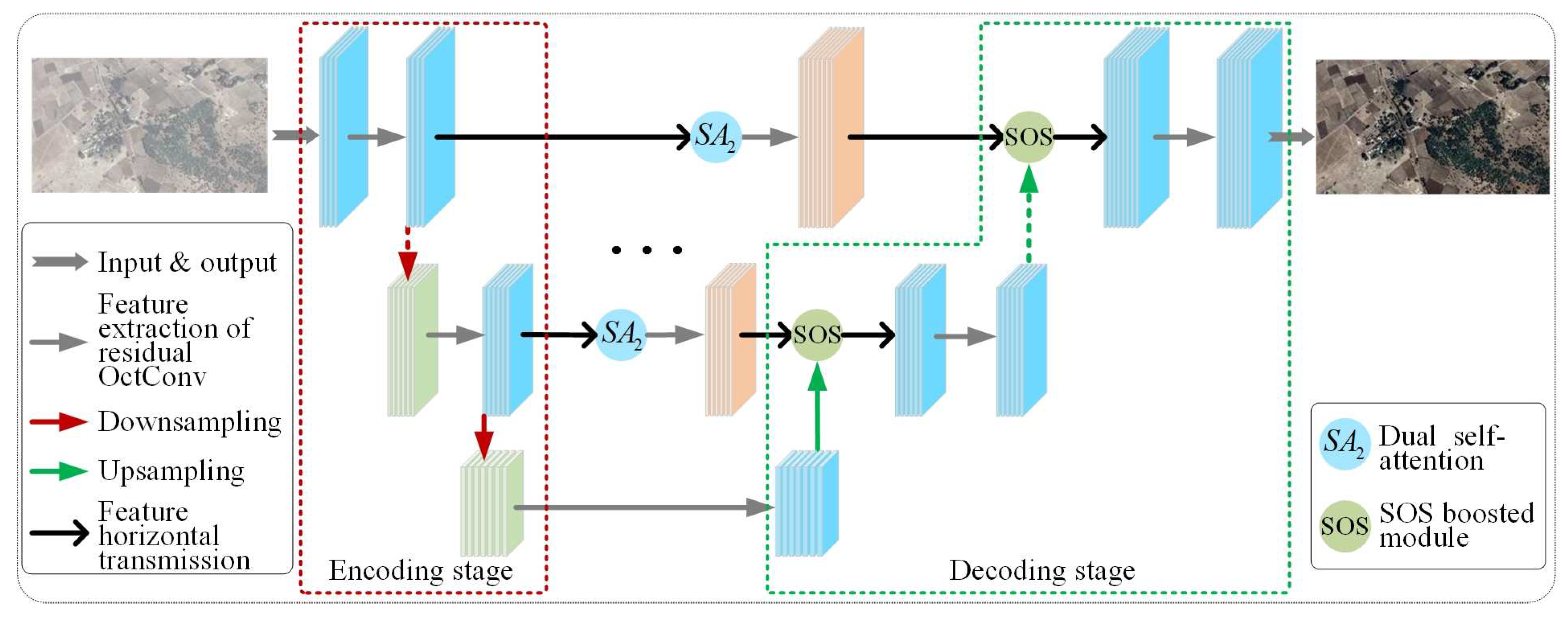
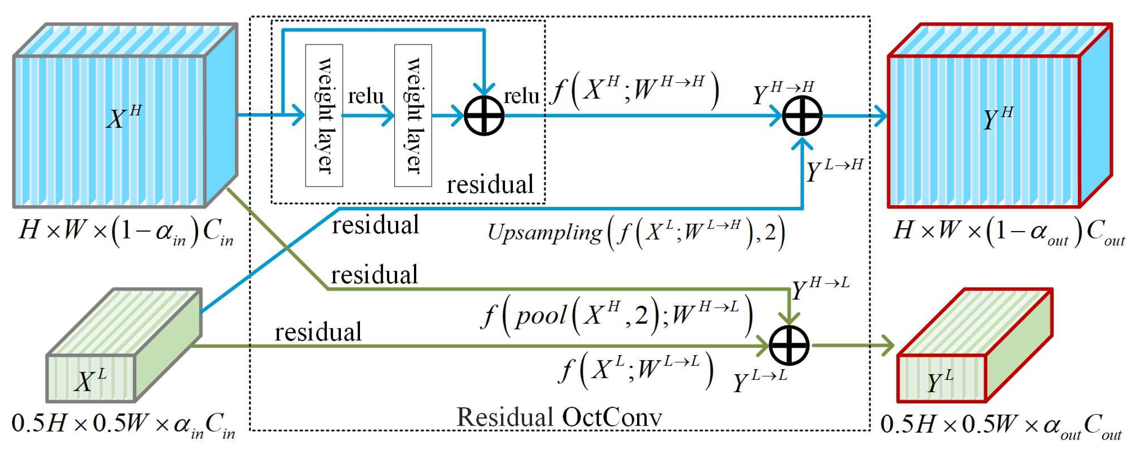
  • This paper proposes remote sensing image defogging backbone networks based on residual octave convolution. Both high-frequency spatial information and low-frequency image information of a foggy remote sensing image can be extracted simultaneously by residual octave convolution. So, the proposed networks can restore both the details of high-frequency components and structure information of low-frequency components, thereby improving the overall quality of the defogged remote sensing image.
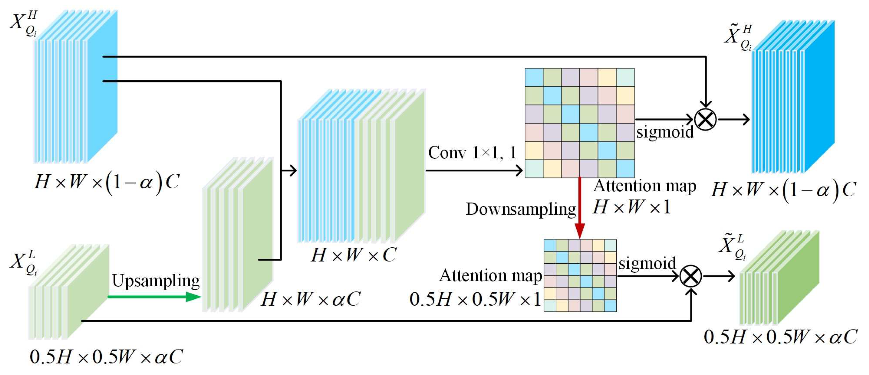
  • This paper proposes a dual self-attention mechanism. Due to the unevenly distributed fog/haze and too much detailed information of a foggy remote sensing image, the proposed dual self-attention mechanism can improve the defogging performance and detail retention ability of the proposed networks in thick fog scenes by paying different attention to different details and different thicknesses of fog.
  • The SOS boosted module is applied to the feature refinement, so the proposed networks can estimate the remote sensing image information and foggy areas separately, which ensures defogging does not destroy the image details and color information during the network transmission process of image features.
The rest of this paper is organized as follows. Section 2 elaborates the proposed method in detail; Section 3 and Section 4 analyze the comparative experimental results; and Section 5 concludes the paper.

2. Methods

This paper proposes a Boost residual octave convolutional remote-sensing image defogging networks based on dual self-attention. As shown in Figure 1, the proposed method uses residual OctConv to extract feature maps. The residual connection method [34] is used to connect the convolutional layers in the octave convolution to form a residual OctConv. In the process of convolution, the octave convolution performs convolution operations in low- and high-frequency flows at the same time [35], which allows the networks to process high- and low-frequency components clearly. This paper improves the process of transferring the feature map of the encoding stage to the decoding stage. Dual self-attention is first used to enhance the feature map; then the SOS boosted module [33] is used to fuse the features of the encoding and decoding stages. The above processes are repeated until the feature fusion result of the last layer is output.

2.1. Feature Map Extraction Based on Residual OctConv

Different from the general convolution, octave convolution considers that the input and output feature maps or channels of the convolutional layer have high- and low-frequency components. The low-frequency components are used to support the overall shape of the object, but they are often redundant, which can be alleviated in the encoding process. The high-frequency components are used to restore the edges (contours) and detailed textures of the original foggy image. In octave convolution, the low-frequency components refer to the feature map obtained after Gaussian filtering processing, and the high-frequency components refer to the original feature map without Gaussian filtering. Due to the redundancy of the low-frequency components, the feature map size of the low-frequency components is set to half the feature map size of the high-frequency components.
The input feature map X and convolution kernel W in the convolutional layer are divided into high- and low-frequency components as follows.
X = X L , X H W = W L , W H
where X L and X H respectively represent the low- and high-frequency components of the feature map. W represents a k × k convolution kernel, W L represents a convolution kernel used for low-frequency components, and W H represents a convolution kernel used for high-frequency components. Residual OctConv performs effective communication between the feature representations of low- and high-frequency components while extracting low-frequency and high-frequency features, as shown in Figure 2. Since the sizes of the high- and low-frequency feature maps are not consistent, the convolution operation cannot be performed. Therefore, in order to achieve effective communication between high- and low-frequency features, it is necessary to upsample the low-frequency components, when the information is updated from low frequency to high frequency (the process W L H ).
Y H = f X H ; W H H + U p s a m p l i n g f X L ; W L H , k
where f X ; W represents the convolution with convolution kernel W parameters. U p s a m p l i n g f · , k represents upsampling, and the calculation is performed according to the nearest interpolation k = 2 .
In the process of W H L , average pooling is applied to downsampling the high-frequency components as follows.
Y L = f X L ; W L L + f p o o l X H , k ; W H L
where p o o l X ; k represents the average pooling operation to achieve downsampling, and the stride k is 2.
The final output is represented by Y H and Y L as follows.
Y = Y L , Y H
where Y H = Y H H + Y L H , and Y L = Y L L + Y H L .

2.2. Feature Enhancement Strategy Based on Dual Self-Attention

Since feature maps obtained after feature extraction by residual OctConv have high- and low-frequency components, this paper performs the feature information fusion on the high- and low-frequency feature maps by dual self-attention. As shown in Figure 3, spatial self-attention [36] is used to enhance the important information in feature maps, and high- and low-frequency components are simultaneously processed in a dual-frequency manner. First, the low-frequency component X Q i L from a certain layer of the encoding stage is upsampled to the same scale as the high-frequency component X Q i H for channel splicing and integration. Then, feature maps are convolved by the convolution kernel with 1 × 1 size to generate a spatial attention weight map. For the high-frequency components of feature maps, the generated attention weight map is first normalized by the sigmoid function, and then directly multiplied with feature maps of the high-frequency components to obtain the high-frequency feature maps X ˜ Q i H enhanced by the spatial self-attention mechanism as follows.
X ˜ Q i H = δ C o n v 1 × 1 X Q i H ; X Q i L X Q i H
where δ · represents the sigmoid function, and C o n v 1 × 1 · represents the convolution of feature maps after channel splicing and fusion with the 1 × 1 convolution kernel size and 1 step size. ⊗ means that the generated attention map is multiplied by the corresponding points of each high-frequency feature map. X Q i H and X Q i L respectively represent the output of the high- and low-frequency components of the i-th layer of the encoding stage.
For the low-frequency components of feature maps, the generated attention map is first downsampled to the same scale as the low-frequency components, and then the sigmoid function is used to normalize it, and finally it is multiplied with the low-frequency components to obtain the low-frequency feature maps X ˜ Q i L enhanced by the spatial self-attention mechanism as follows.
X ˜ Q i L = δ S u b C o n v 1 × 1 X Q i H ; X Q i L X Q i L
where S u b · represents downsampling.
In the above process, the effective communication between low- and high-frequency features is realized. At the same time, the high- and low-frequency feature maps from a certain layer in the encoding stage are transferred to the corresponding layer in the decoding stage after feature enhancement for feature fusion.

2.3. Feature Map Information Fusion Based on SOS Boosted Module

As shown in Figure 4, the SOS boosted module is used to fuse the enhanced feature maps ( X ˜ Q i H , X ˜ Q i L ) passed from the i-th layer of the encoding stage with the feature map ( Y P i + 1 H , Y P i + 1 L ) of the i+1-th layer of the decoding stage.
The i-th layer X ˜ Q i H from the encoding stage is effectively fused with the i + 1-th layer Y P i + 1 H from the decoding stage. Since X ˜ Q i H and Y P i + 1 H have different sizes, upsampling is performed on Y P i + 1 H to keep its size consistent with X ˜ Q i H . The specific process of integration is shown as follows.
X P i H = O c t C o n v X ˜ Q i H + U p Y P i + 1 H U p Y P i + 1 H
where U p · represents upsampling. O c t C o n v · represents the convolution operation. The fusion result X P i H is processed by residual OctConv to obtain the high-frequency feature components Y P i H corresponding to the i-th layer of the decoding stage. Similarly, X P i L is obtained after processing in the SOS Boosted module as follows.
X P i L = O c t C o n v X ˜ Q i L + U p Y P i + 1 L U p Y P i + 1 L
where Y P i L is obtained by applying the convolution operations to X P i L , and Y P i L is the final output of the i-th layer of the decoding stage.
Each layer corresponding to encoding-decoding is processed in the above manner until the last upsampling is completed. The final high- and low-frequency feature maps components Y H and Y L are obtained by applying residual OctConv to the last feature maps processed by the SOS Boosted module. Finally, the fog-free remote sensing image is obtained by outputting the convolution.

2.4. Usage Comparison of SOS between an Existing Method and the Proposed Method

The SOS enhancement strategy proposed in [33] is mainly used to enhance the feature maps that are passed from the encoding stage to the decoding stage. Specifically, the feature maps output by the i-th layer of the coding stage in the network structure are horizontally transferred to the SOS boosted module of the corresponding layer as the feature maps to be enhanced. Additionally, the feature maps from the (i + 1)-th layer of the decoding stage are upsampled and input into the SOS boosted module as latent feature maps. The latent feature maps and the feature maps to be enhanced are first fused at the pixel level to obtain enhanced feature maps. Then, the enhanced feature maps are subjected to a convolution operation to remove the latent feature maps used for enhancement. Finally, refined feature maps are obtained as the output of the SOS boosted module.
In the network structure of the proposed method, feature extraction is performed in the form of dual frequency. For the horizontal output of feature maps in the coding structure, the feature maps first need to highlight the important spatial regions in the feature maps through a dual self-attention mechanism, and then they are input into the SOS boosted module. Next, latent feature maps are used in the SOS Boosted module to perform feature enhancement. Finally, the refined feature maps are output. The dual self-attention highlights the important spatial regions in the feature maps, which is different from [33]. So, the feature enhancement in the SOS boosted module can focus on the feature information on the important spatial regions.

3. Results

3.1. Experiment Preparations

200 fog-free remote sensing images were first collected from Google Earth, and then synthetic fog was added to them by an existing atmospheric scattering model [37] to obtain the training dataset. All image sizes are uniformly scaled to 512 × 512 in the training process. The training of the proposed defogging method was performed on the obtained training dataset. To verify the performance of the proposed defogging method on remote sensing images, 150 remote sensing images (including 100 foggy images and 50 fog-free images) were collected from Google Earth as the testing dataset. The collected sample images include ground vegetation, soil, lakes, swamp, roads, and various buildings. 50 fog-free images are used to obtain synthetic remote sensing images. All the synthetic remote sensing images used in the comparative experiments were synthesized by an existing atmospheric scattering model [37]. Although the proposed method is specialized for remote sensing image defogging, it is also applied to HazeRD dataset [38], which contains 75 synthetic ordinary outdoor foggy images. All 75 foggy images in HazeRD dataset are used as the testing dataset. The defogging performance of the proposed method is compared with the corresponding defogging performance of AMP [6], CAP [15], DCP [12], DehazeNet [26], GPR [39], MAMF [40], RRO [41], WCD [11], and MSBDN [33]. The comparative experiments of the traditional defogging methods were implemented in MATLAB 2016b on a desktop with an Intel(R) Core(TM) i9-7900X @ 3.30 GHz CPU and 16.00 GB RAM. The comparative experiments of the deep learning defogging methods and the proposed method were implemented in Pytorch on a desktop with an NVIDIA 1080Ti GPU, an Intel(R) Core(TM) i9-7900X @ 3.30 GHz CPU, and 16.00 GB RAM.
Four objective evaluation indicators are used to evaluate the defogging performance. Structural similarity (SSIM) is used to evaluate the structural similarity between the defogged synthetic foggy image and original clear image by comparing brightness, contrast, and structure. The larger value of SSIM means the higher similarity between two images [42]. Peak signal-to-noise ratio (PSNR) represents the ratio of the maximum possible power of the signal to the corrosion noise power affecting signal fidelity. The larger value of PSNR means the less distortion of the defogged image [43]. SSIM and PSNR are used to evaluate the defogging performance of synthetic-fog images. Fog aware density evaluator (FADE) is used to evaluate the defogging performance of non-referenced images. The smaller value of FADE means the lower blurriness of the defogged image [44]. Entropy reflects the average amount of information in the image. The larger value of Entropy means the higher average amount of information is retained in the defogged image [45]. FADE and Entropy are used to objectively evaluate the defogged results of real-world foggy images.

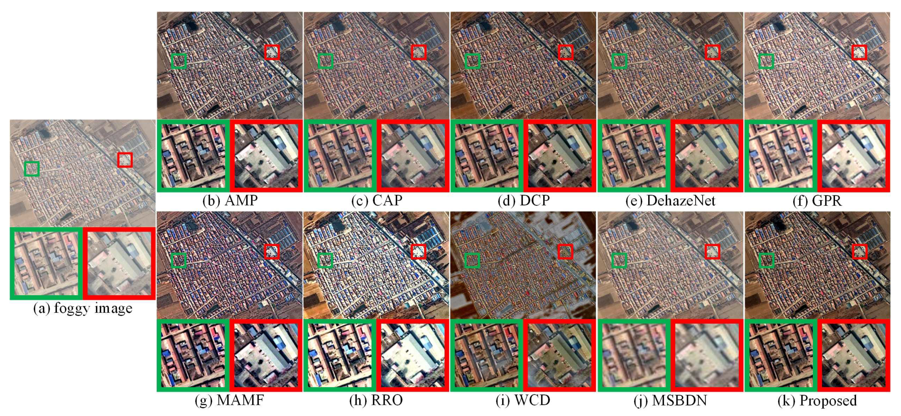
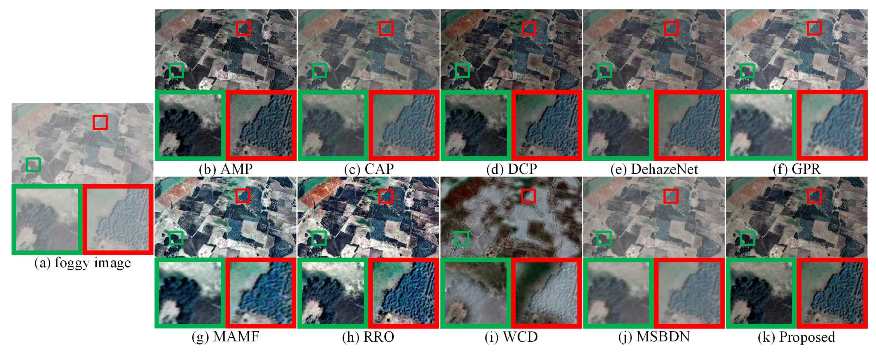
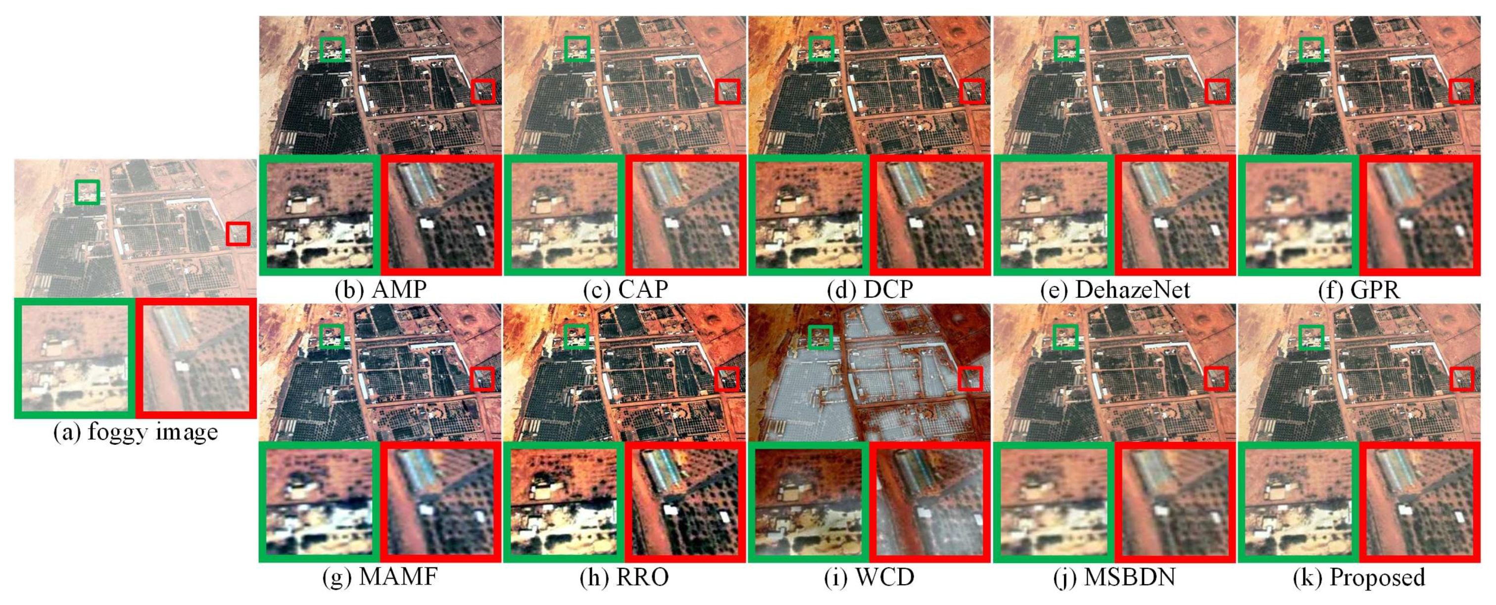
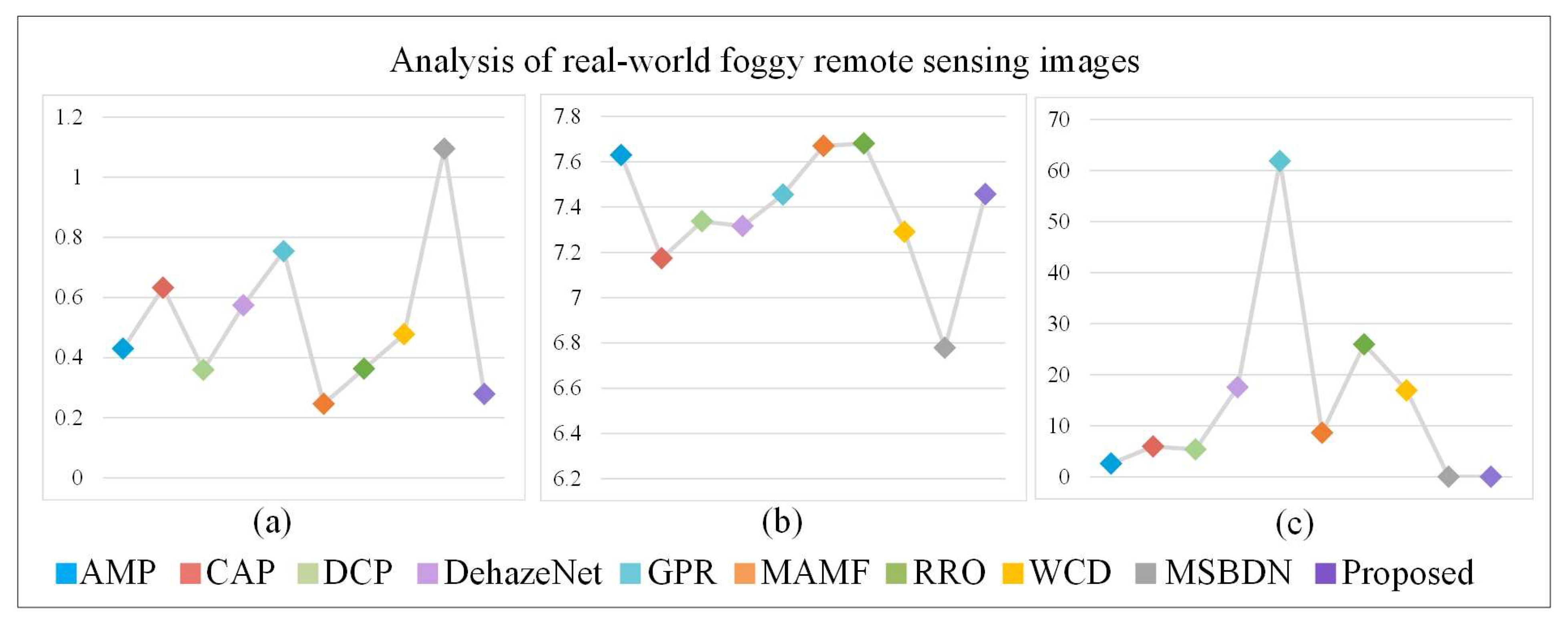
3.2. Results of the Real-World Foggy Remote Sensing Images

Two groups of defogged real-world foggy remote sensing images are selected from 100 groups of comparative experiments for demonstration. Figure 5a shows the original foggy image containing buildings and bare soil. As shown in Figure 5h, the brightness of the defogged image obtained by RRO is too high. Figure 5i shows that the defogged image obtained by WCD has obvious distortion after defogging. The partially enlarged areas of Figure 5c,f show that the detailed textures recovered by CAP and GPR are not clear. As shown in Figure 5g, the saturation of the defogged image obtained by MAMF is high. As shown in Figure 5b, AMP achieved significant defogging performance, but the overall saturation of the defogged image is low. As shown in Figure 5e, the overall saturation of the defogged image obtained by DehazeNet is low, and two partially enlarged images show a small amount of fog residue. As shown in Figure 5d, the brightness of the defogged image obtained by DCP is low. As shown in Figure 5j, the brightness of the defogged image obtained by MSBDN is high and the details of the partially enlarged areas are not clear. The image defogging performance of the proposed method is significant, and the detailed information of the defogged image as shown in the partially enlarged areas of Figure 5k is clear.
The scene in Figure 6a contains densely distributed buildings and bare soil. Figure 6i shows that the defogging performance of WCD is not obvious. As shown in Figure 6f,h, the overall brightness of the defogged images obtained by GPR and RRO is relatively high. The partially enlarged areas of Figure 6f show blurry detailed textures. The overexposure of Figure 6h causes unclear details. As shown in Figure 6j, the defogged image obtained by MSBDN has a small amount of fog residue, and the details of the partially enlarged areas are blurry. As shown in the partially enlarged areas of Figure 6c,e, the fog with low-density distribution exists in the defogged images obtained by CAP and DehazeNet. AMP, DCP, MAMF, and the proposed method achieved effective defogging. Compared with Figure 6b,g, the overall brightness, saturation, and contrast of Figure 6d,k are more in line with the observation habits of human eyes.

3.3. Results of the Synthetic Foggy Remote Sensing Images

Three groups of defogged synthetic foggy remote sensing images are selected from 50 groups of comparative experiments for demonstration. The scene in Figure 7a contains ground vegetation and bare soil. As shown in Figure 7b, AMP achieved significant defogging performance, but the overall saturation of the defogged image is low. As shown in Figure 7c,j, the defogged images obtained by CAP and MSBDN have a small amount of fog residue. As shown in the partially enlarged areas of Figure 7c,j, the details of ground vegetation and bare soil are blurry, and the contrast is low. As shown in Figure 7d, DCP achieved good defogging performance, but the overall brightness of the defogged image is low and fog residue still exists in a small part of the defogged image. As shown in the partially enlarged areas of Figure 7f, the details of the defogged image obtained by GPR are blurry. As shown in Figure 7g,h, the overall brightness of the defogged images obtained by MAMF and RRO is relatively high, and the partially enlarged areas of Figure 7h show that the defogged image is excessively sharpened. As shown in Figure 7i, the defogged image obtained by WCD contains obvious fog residue. Both DehazeNet and the proposed method achieved good defogging performance. As shown in the partially enlarged areas of Figure 7e,k, the detailed information of the defogged image obtained by the proposed method is clearer than the corresponding one obtained by DehazeNet. The overall contrast and saturation of the defogged image obtained by the proposed method are more in line with the observation habits of human eyes.
The scene in Figure 8a contains ground vegetation, bare soil, and buildings. Figure 8i shows that WCD has poor defogging performance. As shown in Figure 8b,g, the saturation of the defogged images obtained by AMP and MAMF is low. As shown in the partially enlarged areas of Figure 8g, MAMF cannot effectively recover the detailed information. As shown in Figure 8d,h, the overall saturation of the defogged images obtained by DCP and RRO is high. RRO also over-sharpened the defogged image shown in Figure 8h. As shown in Figure 8f,j, although GPR and MSBDN achieved good contrast and saturation performance on the defogged images, they cannot effectively restore the detailed textures shown in the partially enlarged areas of the original foggy image. As shown in Figure 8c, the brightness of the defogged image obtained by CAP is high and the contrast is low. As shown in Figure 8e,k, DehazeNet and the proposed method effectively achieved defogging.
The scene in Figure 9a contains buildings and vehicles. As shown in Figure 9f,g, the overall brightness of the defogged images obtained by GPR and MAMF are relatively high, and the detailed textures shown in the corresponding partially enlarged areas is blurry. As shown in Figure 9j, fog was effectively removed by MSBDN, but the details of the partially enlarged areas are not clear. As shown in Figure 9b, AMP can achieve effective defogging, but the brightness of the local details shown in the partially enlarged areas is low. As shown in Figure 9c,e, the defogged images obtained by CAP and DehazeNet contain a small amount of fog residue, and thin haze still exists under the observation of human eyes. As shown in Figure 9d, DCP can recover the detailed textures of the original foggy image, but the overall brightness of the defogged image is low. As shown in Figure 9h, the defogged image obtained by RRO is over-sharpened. Figure 9i shows that WCD cannot achieve effective defogging. As shown in Figure 9k, the proposed method achieved effective defogging of remote sensing images, and restored clear local detailed textures.

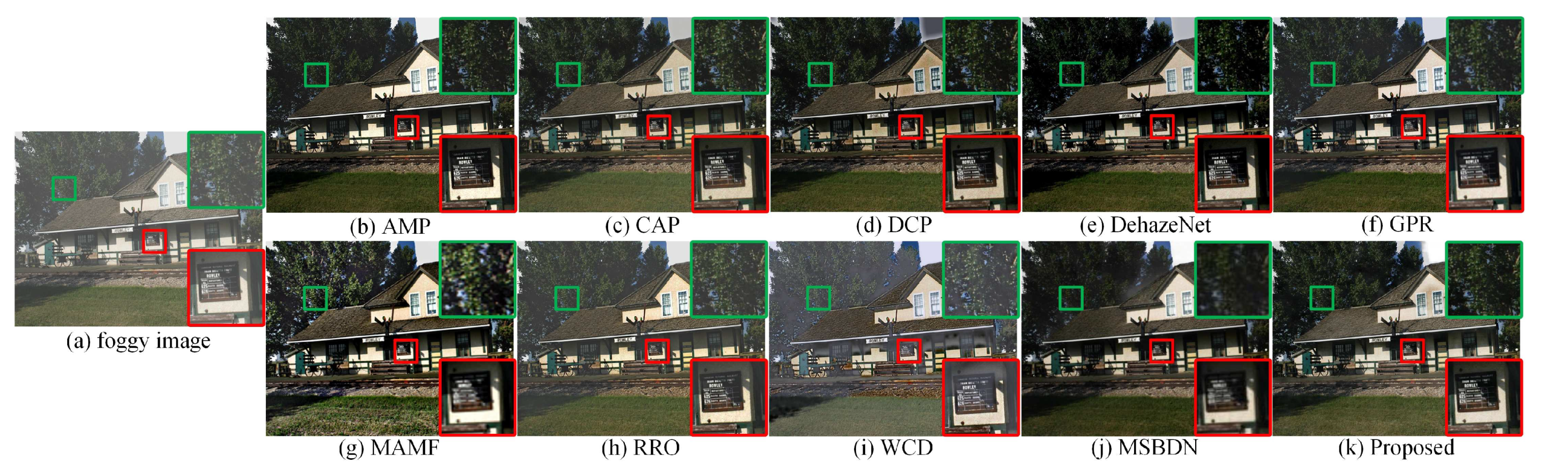
3.4. Results of the Synthetic Foggy Ordinary Outdoor Images

One group of defogged synthetic ordinary outdoor foggy images is selected from 75 groups of comparative experiments on HazeRD dataset for demonstration. Figure 10 compares the defogging performance of ten methods on a synthetic foggy image. As shown in Figure 10i, WCD cannot achieve effective defogging. As shown in Figure 10d, DCP can recover the detailed textures, but the overall brightness of the defogged image is low and the color of sky is distorted. As shown in Figure 10f,g, although GPR and MAMF can achieve effective defogging, the details of the partially enlarged areas are not clear. As shown in Figure 10h, the brightness and contrast of the defogged image obtained by RRO is low. As shown in Figure 10j, the brightness of the defogged image obtained by MSBDN is suitable, but the details of the partially enlarged areas are not clear and a small amount of fog residue exists. As shown in Figure 10b,c,e,k, AMP, CAP, DehazeNet, and the proposed method achieve good defogging performance. Compared with CAP and DehazeNet, the overall brightness of the defogged images obtained by AMP and the proposed method is slightly better. The detailed textures of the partially enlarged areas of the defogged images obtained by AMP, CAP, and the proposed method are slightly better than the one obtained by DehazeNet.

4. Discussion

4.1. Analysis of the Defogged Results of the Real-World Foggy Remote Sensing Images

Three objective evaluation indicators, FADE, Entropy and processing time, are used to evaluate the defogging performance of real-world remote sensing images. Table 1 and Figure 11 show the average FADE, Entropy and processing time of 100 groups of comparative experiments. AMP has a high Entropy value, but its FADE value is also high, which means it does not perform well on defogging. DCP, MAMF, RRO, and the proposed method have low FADE values, which means they achieve effective defogging. However, the average processing time of MAMF and RRO is relatively long. According to the ranking of FADE values, the defogging performance of the proposed method is slightly better than the corresponding ones of DCP and RRO. DCP has a high ranking of FADE value, but its Entropy value ranking is low, which means partial image information is lost in the defogging process. MSBDN has a short average processing time, but its rankings of both Entropy and FADE values are low. The results of FADE, Entropy, and average processing time confirm that the proposed method can achieve good defogging performance.

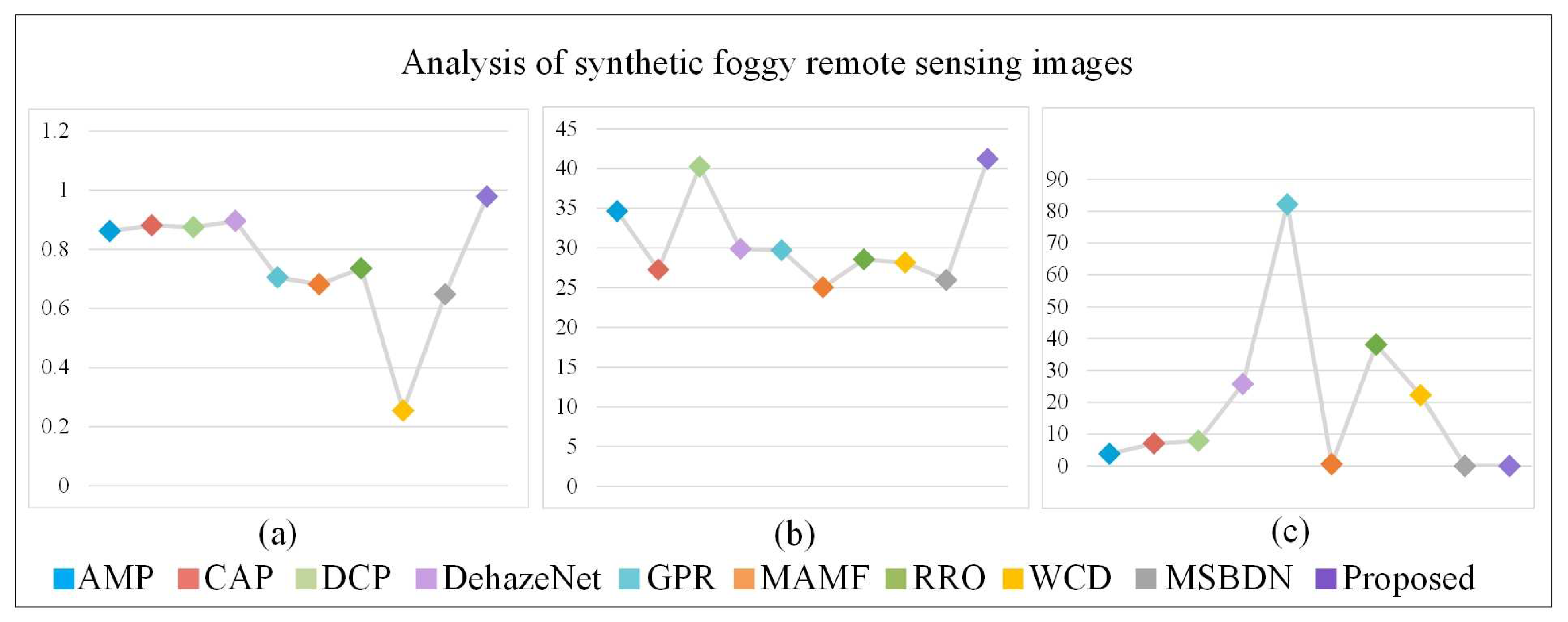
4.2. Analysis of the Defogged Results of the Synthetic Foggy Remote Sensing Images

Three objective evaluation indicators, SSIM, PSNR and processing time, are used to evaluate the defogging performance of synthetic remote sensing images. Table 2 and Figure 12 show the average SSIM, PSNR and processing time of 50 groups of comparative experiments. CAP, DehazeNet, DCP and the proposed method have high SSIM value, which means they effectively retain the structural information of the original foggy images. The structure of the defogged images obtained by CAP, DehazeNet, DCP and the proposed method is highly similar to the structure of the original foggy image. AMP, DehazeNet and DCP obtain high PSNR values, so the quality of the defogged images obtained by them is high. However, the SSIM value of AMP is relatively low, which indicates that the defogged image obtained by AMP cannot effectively retain the structural information of the original foggy image. Although the SSIM value of CAP is relatively high, its PSNR value is relatively low, which means the defogging performance of CAP is not good. MSBDN has the lowest average processing time, but its rankings of SSIM and PSNR values are low, which means the defogged image obtained by MSBDN cannot effectively retain the structural information of the original foggy image and partial image information is lost in the defogging process. The proposed method obtains the highest values on both SSIM and PSNR, which means the proposed method can effectively restore the structural information of the original foggy images with the least distortion.

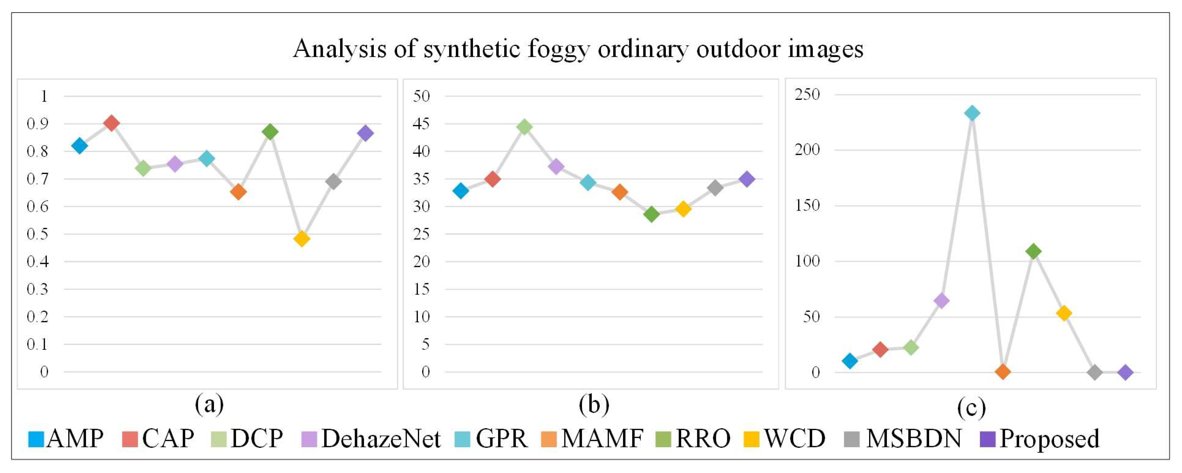
4.3. Analysis of the Defogged Results of the Synthetic Foggy Ordinary Outdoor Images

SSIM, PSNR and processing time are used to evaluate the defogging performance of synthetic foggy images from HazeRD dataset. Table 3 and Figure 13 show the average SSIM, PSNR and processing time of comparative experiments. CAP, DCP, DehazeNet, and the proposed method obtain the top four highest PSNR values, which means the quality of the defogged images obtained is high. Although the PSNR values obtained by DCP and DehazeNet are relatively high, their SSIM values are relatively low, which means the defogged images obtained cannot effectively retain the structural information of the original foggy image. The SSIM values obtained by AMP and RRO are relatively high, but their PSNR values are relatively low, which means the defogged images obtained contain distortion. Although CAP and the proposed method can effectively retain the structural information and reduce image distortion, the average processing time of CAP is relatively long. The average processing time of MSBDN is short, but its rankings of SSIM and PSNR values are low. The comparative results confirm the proposed method achieved the best overall performance with the least processing time.

4.4. Ablation Study

Ablation study is performed on the synthetic foggy remote sensing images to evaluate the contributions of each module.
Figure 14 and Table 4 show the results of ablation study. The baseline is the encoding-decoding structure with residual OctConv. The synthetic foggy remote sensing images are directly input into the baseline. The SSIM and PSNR of baseline are 0.6220 and 24.0683, respectively. A represents SOS boosted module. The fusion of feature maps is added to the baseline, which greatly improves the defogging performance of the baseline. The SSIM and PSNR of baseline + A are improved by 0.334 and 10.9363, respectively. According to Figure 14c,d, the contour, details, textures, and other information of the foggy image can be further restored through the effective fusion of features. B represents dual self-attention. The defogging performance of baseline + A is further improved by applying dual self-attention to feature maps. Compared with baseline + A, the SSIM and PSNR of baseline + A + B are improved by 0.0229 and 6.1755, respectively. As shown in Figure 14b,d,e, the detailed information of the defogged image is further optimized after feature enhancement. So, dual self-attention makes the color of the defogged image closer to the color of the original fog-free image. Overall, three parts of the proposed networks working together can achieve good defogging performance.

4.5. Experiment Results Discussion

This paper evaluates the proposed defogging method from subjective and objective aspects. The proposed method achieved good performance in both subjective and objective evaluations. In general, the visual effects of the defogged images obtained by the proposed method are more in line with the observation habits of human eyes, and the proposed method is suitable for various complex scenes and complex situations with different fog density distributions. The proposed method can achieve effective defogging. During the defogging process, the structural information of the original foggy image is effectively restored and the average processing time of the proposed method is relatively short. Additionally, the defogged images obtained by the proposed method retain as much information of the original images as possible with less distortion. The ablation study shows the importance of each part producing good defogging performance.

5. Conclusions

This paper proposes remote sensing image defogging networks based on dual self-attention boost residual octave convolution (DOC). First, residual OctConv is used to extract the high- and low-frequency components of feature maps and also carry out information interaction on the high- and low-frequency components in the meantime. Then, dual self-attention is proposed to enhance the features of high- and low-frequency components; Finally, the SOS boosted module is used to realize the effective fusion of the output of a certain layer of dual self-attention and the feature maps of the next layer of the decoding stage corresponding to the certain layer. The above processes are repeated until the final decoding is completed. The processed feature maps are used to obtain the defogged remote sensing image by convolution. Experimental results confirm that the proposed method can achieve effective defogging, and the defogged images obtained by the proposed method have good visual effects in human visual perception. According to the subjective and objective evaluations of both real-world and synthetic foggy images, the overall defogging performance of the proposed method is better than the corresponding defogging performance of other existing defogging methods. The proposed method is not only suitable for various complex remote sensing scenes, but also is able to restore the structural and detailed information of the original foggy images.

Author Contributions

Conceptualization, Z.Z. and Y.L. (Yong Li); Funding acquisition, Z.Z.; Investigation, Y.L. (Yaqin Luo); Methodology, G.Q.; Software, J.M.; Supervision, N.M. All authors have read and agreed to the published version of the manuscript.

Funding

This work is jointly supported bythe National Natural Science Foundation of China under Grant No. 61803061, 61906026, 61771081; Innovation research group of universities in Chongqing; the Chongqing Natural Science Foundation under Grant cstc2020jcyj-msxmX0577, cstc2020jcyj-msxmX0634, cstc2019jcyj-msxmX0110; “Chengdu-Chongqing Economic Circle” innovation funding of Chongqing Municipal Education Commission KJCXZD2020028; the Science and Technology Research Program of Chongqing Municipal Education Commission grants KJQN202000602; Ministry of Education China Mobile Research Fund (MCM 20180404); Special key project of Chongqing technology innovation and application development: cstc2019jscx-zdztzx0068.

Institutional Review Board Statement

Not applicable.

Informed Consent Statement

Not applicable.

Data Availability Statement

The data that used in this study can be requested by contacting the first author or corresponding author.

Conflicts of Interest

The authors declare no conflict of interest.

References

  1. Li, Y.; Zhang, Y.; Huang, X.; Ma, J. Learning Source-Invariant Deep Hashing Convolutional Neural Networks for Cross-Source Remote Sensing Image Retrieval. IEEE Trans. Geosci. Remote Sens. 2018, 56, 6521–6536. [Google Scholar] [CrossRef]
  2. Guo, J.; Ren, H.; Zheng, Y.; Nie, J.; Chen, S.; Sun, Y.; Qin, Q. Identify Urban Area From Remote Sensing Image Using Deep Learning Method. In Proceedings of the IGARSS 2019—2019 IEEE International Geoscience and Remote Sensing Symposium, Yokohama, Japan, 28 July–2 August 2019; pp. 7407–7410. [Google Scholar]
  3. Zhu, Z.; Wei, H.; Hu, G.; Li, Y.; Qi, G.; Mazur, N. A Novel Fast Single Image Dehazing Algorithm Based on Artificial Multiexposure Image Fusion. IEEE Trans. Instrum. Meas. 2021, 70, 1–23. [Google Scholar]
  4. Liu, Y.; Chen, X.; Ward, R.K.; Jane Wang, Z. Image Fusion With Convolutional Sparse Representation. IEEE Signal Process. Lett. 2016, 23, 1882–1886. [Google Scholar] [CrossRef]
  5. Zheng, M.; Qi, G.; Zhu, Z.; Li, Y.; Wei, H.; Liu, Y. Image Dehazing by an Artificial Image Fusion Method Based on Adaptive Structure Decomposition. IEEE Sens. J. 2020, 20, 8062–8072. [Google Scholar] [CrossRef]
  6. Salazar-Colores, S.; Cruz-Aceves, I.; Ramos-Arreguin, J.M. Single image dehazing using a multilayer perceptron. J. Electron. Imaging 2018, 27, 043022. [Google Scholar] [CrossRef]
  7. Li, W.; Wei, H.; Qi, G.; Ding, H.; Li, K. A Fast Image Dehazing Algorithm for Highway Tunnel Based on Artificial Multi-exposure Image Fusion. IOP Conf. Ser. Mater. Sci. Eng. 2020, 741, 012038. [Google Scholar] [CrossRef] [Green Version]
  8. Zhan, J.; Gao, Y.; Liu, X. Measuring the optical scattering characteristics of large particles in visible remote sensing. In Proceedings of the 2017 IEEE International Geoscience and Remote Sensing Symposium (IGARSS), Fort Worth, TX, USA, 23–28 July 2017; pp. 4666–4669. [Google Scholar]
  9. Du, Y.; Guindon, B.; Cihlar, J. Haze detection and removal in high resolution satellite image with wavelet analysis. IEEE Trans. Geosci. Remote Sens. 2002, 40, 210–217. [Google Scholar]
  10. Shen, H.; Li, H.; Qian, Y.; Zhang, L.; Yuan, Q. An effective thin cloud removal procedure for visible remote sensing images. ISPRS J. Photogramm. Remote Sens. 2014, 96, 224–235. [Google Scholar] [CrossRef]
  11. Chiang, J.Y.; Chen, Y.C. Underwater Image Enhancement by Wavelength Compensation and Dehazing. IEEE Trans. Image Process. 2012, 21, 1756–1769. [Google Scholar] [CrossRef] [PubMed]
  12. He, K.; Sun, J.; Tang, X. Single image haze removal using dark channel prior. In Proceedings of the 2009 IEEE Conference on Computer Vision and Pattern Recognition (CVPR), Miami, FL, USA, 20–25 June 2009; pp. 1956–1963. [Google Scholar]
  13. Long, J.; Shi, Z.; Tang, W. Fast haze removal for a single remote sensing image using dark channel prior. In Proceedings of the 2012 International Conference on Computer Vision in Remote Sensing, Xiamen, China, 16–18 December 2012; pp. 132–135. [Google Scholar]
  14. Xie, F.; Chen, J.; Pan, X.; Jiang, Z. Adaptive Haze Removal for Single Remote Sensing Image. IEEE Access 2018, 6, 67982–67991. [Google Scholar] [CrossRef]
  15. Zhu, Q.; Mai, J.; Shao, L. A Fast Single Image Haze Removal Algorithm Using Color Attenuation Prior. IEEE Trans. Image Process. 2015, 24, 3522–3533. [Google Scholar] [PubMed] [Green Version]
  16. Long, J.; Shi, Z.; Tang, W.; Zhang, C. Single Remote Sensing Image Dehazing. IEEE Geosci. Remote Sens. Lett. 2014, 11, 59–63. [Google Scholar] [CrossRef]
  17. Pan, X.; Xie, F.; Jiang, Z.; Yin, J. Haze Removal for a Single Remote Sensing Image Based on Deformed Haze Imaging Model. IEEE Signal Process. Lett. 2015, 22, 1806–1810. [Google Scholar] [CrossRef]
  18. Singh, D.; Kumar, V. Dehazing of remote sensing images using fourth-order partial differential equations based trilateral filter. IET Comput. Vis. 2017, 12, 208–219. [Google Scholar] [CrossRef]
  19. Liu, Q.; Gao, X.; He, L.; Lu, W. Haze removal for a single visible remote sensing image. Signal Process. 2017, 137, 33–43. [Google Scholar] [CrossRef]
  20. Chen, Y.; Tu, Z.; Ge, L.; Zhang, D.; Chen, R.; Yuan, J. SO-HandNet: Self-Organizing Network for 3D Hand Pose Estimation With Semi-Supervised Learning. In Proceedings of the 2019 IEEE/CVF International Conference on Computer Vision (ICCV), Seoul, Korea, 27–28 October 2019; pp. 6960–6969. [Google Scholar]
  21. Wang, K.; Zheng, M.; Wei, H.; Qi, G.; Li, Y. Multi-Modality Medical Image Fusion Using Convolutional Neural Network and Contrast Pyramid. Sensors 2020, 20, 2169. [Google Scholar] [CrossRef] [PubMed] [Green Version]
  22. Tu, Z.; Xie, W.; Dauwels, J.; Li, B.; Yuan, J. Semantic Cues Enhanced Multimodality Multistream CNN for Action Recognition. IEEE Trans. Circuits Syst. Video Technol. 2019, 29, 1423–1437. [Google Scholar] [CrossRef]
  23. Qi, G.; Wang, H.; Haner, M.; Weng, C.; Chen, S.; Zhu, Z. Convolutional neural network based detection and judgement of environmental obstacle in vehicle operation. CAAI Trans. Intell. Technol. 2019, 4, 80–91. [Google Scholar] [CrossRef]
  24. Liu, Y.; Chen, X.; Wang, Z.; Wang, Z.J.; Ward, R.K.; Wange, X. Deep learning for pixel-level image fusion: Recent advances and future prospects. Inf. Fusion 2018, 42, 158–173. [Google Scholar]
  25. Jiang, H.; Lu, N. Multi-scale residual convolutional neural network for haze removal of remote sensing images. Remote Sens. 2018, 10, 945. [Google Scholar] [CrossRef] [Green Version]
  26. Cai, B.; Xu, X.; Jia, K.; Qing, C.; Tao, D. DehazeNet: An End-to-End System for Single Image Haze Removal. IEEE Trans. Image Process. 2016, 25, 5187–5198. [Google Scholar] [CrossRef] [PubMed] [Green Version]
  27. Zhang, H.; Patel, V.M. Densely Connected Pyramid Dehazing Network. In Proceedings of the 2018 IEEE/CVF Conference on Computer Vision and Pattern Recognition (CVPR), Salt Lake City, UT, USA, 18–23 June 2018; pp. 3194–3203. [Google Scholar]
  28. Li, B.; Peng, X.; Wang, Z.; Xu, J.; Feng, D. AOD-Net: All-in-One Dehazing Network. In Proceedings of the 2017 IEEE International Conference on Computer Vision (ICCV), Venice, Italy, 22–29 October 2017; pp. 4780–4788. [Google Scholar]
  29. Ren, W.; Ma, L.; Zhang, J.; Pan, J.; Cao, X.; Liu, W.; Yang, M.H. Gated Fusion Network for Single Image Dehazing. In Proceedings of the 2018 IEEE/CVF Conference on Computer Vision and Pattern Recognition (CVPR), Salt Lake City, UT, USA, 18–22 June 2018; pp. 3253–3261. [Google Scholar]
  30. Chen, D.; He, M.; Fan, Q.; Liao, J.; Zhang, L.; Hou, D.; Yuan, L.; Hua, G. Gated Context Aggregation Network for Image Dehazing and Deraining. In Proceedings of the 2019 IEEE Winter Conference on Applications of Computer Vision (WACV), Waikoloa, HI, USA, 7–11 January 2019; pp. 1375–1383. [Google Scholar]
  31. Engin, D.; Genc, A.; Ekenel, H.K. Cycle-Dehaze: Enhanced CycleGAN for Single Image Dehazing. In Proceedings of the 2018 IEEE/CVF Conference on Computer Vision and Pattern Recognition Workshops (CVPRW), Salt Lake City, UT, USA, 18–22 June 2018; pp. 938–9388. [Google Scholar]
  32. Pan, J.; Liu, S.; Sun, D.; Zhang, J.; Liu, Y.; Ren, J.; Li, Z.; Tang, J.; Lu, H.; Tai, Y.W.; et al. Learning Dual Convolutional Neural Networks for Low-Level Vision. In Proceedings of the 2018 IEEE/CVF Conference on Computer Vision and Pattern Recognition (CVPR), Salt Lake City, UT, USA, 18–23 June 2018; pp. 3070–3079. [Google Scholar]
  33. Dong, H.; Pan, J.; Xiang, L.; Hu, Z.; Zhang, X.; Wang, F.; Yang, M.H. Multi-Scale Boosted Dehazing Network With Dense Feature Fusion. In Proceedings of the 2020 IEEE/CVF Conference on Computer Vision and Pattern Recognition (CVPR), Seattle, WA, USA, 14–19 June 2020; pp. 2154–2164. [Google Scholar]
  34. He, K.; Zhang, X.; Ren, S.; Sun, J. Deep residual learning for image recognition. In Proceedings of the IEEE Conference on Computer Vision and Pattern Recognition (CVPR), Las Vegas, NV, USA, 27–30 June 2016; pp. 770–778. [Google Scholar]
  35. Chen, Y.; Fan, H.; Xu, B.; Yan, Z.; Kalantidis, Y.; Rohrbach, M.; Shuicheng, Y.; Feng, J. Drop an Octave: Reducing Spatial Redundancy in Convolutional Neural Networks With Octave Convolution. In Proceedings of the 2019 IEEE/CVF International Conference on Computer Vision (ICCV), Seoul, Korea, 27 October–2 November 2019; pp. 3434–3443. [Google Scholar]
  36. Woo, S.; Park, J.; Lee, J.Y.; Kweon, I.S. Cbam: Convolutional block attention module. In Proceedings of the European Conference on Computer Vision (ECCV), Munich, Germany, 8–14 September 2018; pp. 3–19. [Google Scholar]
  37. Nayar, S.K.; Narasimhan, S.G. Vision in bad weather. In Proceedings of the Seventh IEEE International Conference on Computer Vision (ICCV), Kerkyra, Greece, 20–27 September 1999; Volume 2, pp. 820–827. [Google Scholar]
  38. Zhang, Y.; Ding, L.; Sharma, G. HazeRD: An outdoor scene dataset and benchmark for single image dehazing. In Proceedings of the 2017 IEEE International Conference on Image Processing (ICIP), Beijing, China, 17–20 September 2017; pp. 3205–3209. [Google Scholar]
  39. Fan, X.; Wang, Y.; Tang, X.; Gao, R.; Luo, Z. Two-Layer Gaussian Process Regression With Example Selection for Image Dehazing. IEEE Trans. Circuits Syst. Video Technol. 2017, 27, 2505–2517. [Google Scholar] [CrossRef]
  40. Cho, Y.; Jeong, J.; Kim, A. Model-Assisted Multiband Fusion for Single Image Enhancement and Applications to Robot Vision. IEEE Robot. Autom. Lett. 2018, 3, 2822–2829. [Google Scholar]
  41. Shin, J.; Kim, M.; Paik, J.; Lee, S. Radiance-Reflectance Combined Optimization and Structure-Guided l0-Norm for Single Image Dehazing. IEEE Trans. Multimed. 2019, 22, 30–44. [Google Scholar] [CrossRef]
  42. Wang, Z.; Bovik, A.; Sheikh, H.; Simoncelli, E. Image quality assessment: From error visibility to structural similarity. IEEE Trans. Image Process. 2004, 13, 600–612. [Google Scholar] [CrossRef] [Green Version]
  43. Hore, A.; Ziou, D. Image quality metrics: PSNR vs. SSIM. In Proceedings of the International Conference on Pattern Recognition, Istanbul, Turkey, 23–26 August 2010; pp. 2366–2369. [Google Scholar]
  44. Choi, L.K.; You, J.; Bovik, A.C. Referenceless Prediction of Perceptual Fog Density and Perceptual Image Defogging. IEEE Trans. Image Process. 2015, 24, 3888–3901. [Google Scholar] [CrossRef] [PubMed]
  45. Qing, C.; Yu, F.; Xu, X.; Huang, W.; Jin, J. Underwater video dehazing based on spatial–temporal information fusion. Multidimens. Syst. Signal Process. 2016, 27, 909–924. [Google Scholar] [CrossRef]
Figure 1. Overall network architecture. The networks have four downsamplings and four upsamplings in total. In each layer of encoding and decoding (in the first four layers of the networks), the feature maps of the encoding stage are passed to the decoding stage in the same way. The feature map of each layer of encoding stage is first processed by dual self-attention to obtain the feature map after feature enhancement, and then the feature map and the feature map in the decoding stage of the next layer after upsampling are input into the SOS boosted module, thereby realizing the effective fusion of image feature information. The feature transfer method of encoding-decoding in the last layer is only processed by convolution operations. The fused feature map is sent to the next convolution operation and then upsampled. Finally, the feature map after the last feature fusion is restored to a fog-free image.
Remotesensing 13 03104 g001
Figure 2. Residual OctConv performs feature map extraction and information communication in dual frequency (high frequency and low frequency). In the entire network framework, the first and last convolutions of the network are set to α i n = 0 , α o u t = α and α i n = α , α o u t = 0 . The other convolutional layers are set to α i n = α o u t = α . The ratio of high-frequency components to low-frequency components is set to 1 : 1 , so the value of α is 0.5. The feature map size of the low-frequency components is set to half the feature map size of the high-frequency components, so its size is 0.5 H × 0.5 W .
Remotesensing 13 03104 g002
Figure 3. Dual self-attention. The high- and low-frequency components are first used to jointly generate the attention weight map, and then the generated attention weight map are multiplied by the high- and low-frequency components to obtain feature maps after feature enhancement. The feature map size of the low-frequency components is set to half the feature map size of the high-frequency components, so its size is 0.5 H × 0.5 W .
Remotesensing 13 03104 g003
Figure 4. SOS Boosted module. This module achieves the effective feature fusion on the output of the i-th layer from the encoding stage and the upsampling result of the i + 1-th layer from the decoding stage. (a,b) are performed simultaneously in a residual OctConv. For the feature maps of the i-th layer, the feature map size of X ˜ Q i L is set to the half size of X ˜ Q i H , so its size is 0.5 H × 0.5 W . Y P i + 1 H represents the high-frequency components from the i + 1-th layer and its size is 0.5 H × 0.5 W . Y P i + 1 L represents the low-frequency components from the i + 1-th layer and its size is 0.25 H × 0.25 W .
Remotesensing 13 03104 g004
Figure 5. (a) shows a real-world foggy remote sensing image. (bk) respectively represent the defogged images obtained by AMP, CAP, DCP, DehazeNet, GPR, MAMF, RRO, WCD, MSBDN, and the proposed method. The two partially enlarged images marked in the green and red frames correspond to two areas enclosed by the green and red frames in each defogged image.
Remotesensing 13 03104 g005
Figure 6. (a) shows a real-world foggy remote sensing image. (bk) respectively represent the defogged images obtained by AMP, CAP, DCP, DehazeNet, GPR, MAMF, RRO, WCD, MSBDN, and the proposed method. The two partially enlarged images marked in the green and red frames correspond to two areas enclosed by the green and red frames in each defogged image.
Remotesensing 13 03104 g006
Figure 7. (a) shows a synthetic foggy remote sensing image. (bk) respectively represent the defogged images obtained by AMP, CAP, DCP, DehazeNet, GPR, MAMF, RRO, WCD, MSBDN, and the proposed method. The two partially enlarged images marked in the green and red frames correspond to two areas enclosed by the green and red frames in each defogged image.
Remotesensing 13 03104 g007
Figure 8. (a) shows a synthetic foggy remote sensing image. (bk) respectively represent the defogged images obtained by AMP, CAP, DCP, DehazeNet, GPR, MAMF, RRO, WCD, MSBDN, and the proposed method. The two partially enlarged images marked in the green and red frames correspond to two areas enclosed by the green and red frames in each defogged image.
Remotesensing 13 03104 g008
Figure 9. (a) shows a synthetic foggy remote sensing image. (bk) respectively represent the defogged images obtained by AMP, CAP, DCP, DehazeNet, GPR, MAMF, RRO, WCD, MSBDN, and the proposed method. The two partially enlarged images marked in the green and red frames correspond to two areas enclosed by the green and red frames in each defogged image.
Remotesensing 13 03104 g009
Figure 10. (a) shows a synthetic foggy image from HazeRD dataset. (bk) respectively represent the defogged images obtained by AMP, CAP, DCP, DehazeNet, GPR, MAMF, RRO, WCD, MSBDN, and the proposed method. The two partially enlarged images marked in the green and red frames correspond to two areas enclosed by the green and red frames in each defogged image.
Remotesensing 13 03104 g010
Figure 11. Analysis of ten image defogging methods in real-world foggy remote sensing scenes, (a) FADE, (b) Entropy, (c) processing time.
Remotesensing 13 03104 g011
Figure 12. Analysis of ten image defogging methods in synthetic foggy remote sensing scenes, (a) SSIM, (b) PSNR, (c) processing time.
Remotesensing 13 03104 g012
Figure 13. Analysis of ten image defogging methods in synthetic foggy ordinary outdoor scenes, (a) SSIM, (b) PSNR, (c) processing time.
Remotesensing 13 03104 g013
Figure 14. Results of ablation study. (a) shows the synthetic foggy remote sensing image; (b) shows the original fog-free remote sensing image; (c) shows the defogged image obtained by baseline; (d) shows the defogged image obtained by baseline + A; (e) shows the defogged image obtained by baseline + A + B.
Remotesensing 13 03104 g014
Table 1. Analysis of the defogging performance of the real-world foggy remote sensing images using three evaluation indicators. The top four results are marked in bold, and the corresponding rankings are shown in parentheses. The lower FADE value is better, the higher Entropy value is better.
AMPCAPDCPDehazeNetGPRMAMFRROWCDMSBDNProposed
FADE0.43000.63230.3589(3)0.57370.75380.2460(1)0.3633(4)0.47751.09470.2783(2)
Entropy7.6292(3)7.17427.33707.31627.45547.6697(2)7.6810(1)7.29076.77907.4568(4)
Time(s)2.6193(3)5.93255.3533(4)17.556461.85048.648925.944116.95510.0304(2)0.0253(1)
Table 2. Analysis of the defogging performance of the synthetic foggy remote sensing images using three evaluation indicators. The top four results are marked in bold, and the corresponding rankings are shown in parentheses. The higher SSIM and PSNR values are better.
AMPCAPDCPDehazeNetGPRMAMFRROWCDMSBDNProposed
SSIM0.86230.8817(3)0.8751(4)0.8960(2)0.70520.68180.73580.25460.64850.9789(1)
PSNR34.6232(3)27.266040.2194(2)29.8736(4)29.708925.063028.542428.151725.968741.1801(1)
Time(s)3.8334(4)7.09327.860825.757882.09110.6135(3)38.147922.23660.0413(1)0.0424(2)
Table 3. Analysis of the defogging performance of the synthetic foggy images from HazeRD dataset using three evaluation indicators. The top four results are marked in bold, and the corresponding rankings are shown in parentheses. The higher SSIM and PSNR values are better.
AMPCAPDCPDehazeNetGPRMAMFRROWCDMSBDNProposed
SSIM0.8202(4)0.9027(1)0.73850.75410.77370.65310.8712(2)0.48250.69010.8661(3)
PSNR32.820034.9427(4)44.4166(1)37.2500(2)34.312832.606128.564629.541833.378734.9675(3)
Time(s)10.2798(4)20.564622.404464.5915233.35490.7154(3)108.949653.42610.0333(2)0.0315(1)
Table 4. Results of ablation study. Baseline is the encoding-decoding structure with residual OctConv. A represents SOS boosted module. B represents dual self-attention.
SSIMPSNR
baseline0.622024.0683
baseline + A0.956035.0046
baseline + A + B0.978941.1801
Publisher’s Note: MDPI stays neutral with regard to jurisdictional claims in published maps and institutional affiliations.

