Abstract
The relevant benefits of hyperspectral sensors for water column determination and seabed features mapping compared to multispectral data, especially in coastal areas, have been demonstrated in recent studies. In this study, we used hyperspectral satellite data in the accurate mapping of the bathymetry and the composition of water habitats for inland water. Particularly, the identification of the bottom diversity for a shallow lagoon (less than 2 m in depth) was examined. Hyperspectral satellite data were simulated based on aerial hyperspectral imagery acquired above a lagoon, namely the Vaccarès lagoon (France), considering the spatial and spectral resolutions, and the signal-to-noise ratio of a satellite sensor, BIODIVERSITY, that is under study by the French space agency (CNES). Various sources of uncertainties such as inter-band calibration errors and atmospheric correction were considered to make the dataset realistic. The results were compared with a recently launched hyperspectral sensor, namely the DESIS sensor (DLR, Germany). The analysis of BIODIVERSITY-like sensor simulated data demonstrated the feasibility to satisfactorily estimate the bathymetry with a root-mean-square error of 0.28 m and a relative error of 14% between 0 and 2 m. In comparison to open coastal waters, the retrieval of bathymetry is a more challenging task for inland waters because the latter usually shows a high abundance of hydrosols (phytoplankton, SPM, and CDOM). The retrieval performance of seabed abundance was estimated through a comparison of the bottom composition with in situ data that were acquired by a recently developed imaging camera (SILIOS Technologies SA., France). Regression coefficients for the retrieval of the fractional species abundances from the theoretical inversion and measurements were obtained to be 0.77 (underwater imaging camera) and 0.80 (in situ macrophytes data), revealing the potential of the sensor characteristics. By contrast, the comparison of the in situ bathymetry and macrophyte data with the DESIS inverted data showed that depth was estimated with an RSME of 0.38 m and a relative error of 17%, and the fractional species abundance was estimated to have a regression coefficient of 0.68.
1. Introduction
Shallow coastal and inland water ecosystems have substantial roles in the environment and economy [1,2]. These ecosystems have undergone high stress from anthropogenic activities, resulting in dramatic changes in the functioning of ecosystems, habitat structure, and species composition [3,4,5]. One of the key factors affecting benthic species distribution in lagoons may be the movement of seafloor sediments due to anthropogenic factors [6,7]. In pristine lagoons, water depth and transparency, and hydrology and salinity are key interacting abiotic variables that control the species composition of the vegetation [3,8,9]. From a physical perspective, lagoons are characterized by the coexistence of boundaries and ecological gradients between terrestrial, aquatic, freshwater, and marine environments, as well as strong interactions between water and sediment often mediated by wind action. These interactions characterize lagoon dynamic ecosystems by frequent environmental disturbances and environmental fluctuations [3,10]. Anthropogenic pressures on their catchments often result in eutrophication, affecting their productivity, the transparency of water, and sediment chemistry by the accumulation of organic matter, resulting in shifts in plant community structure and species composition [11,12,13].
Hyperspectral remotely sensed data are relevant to study such complex and dynamic ecosystems [14,15,16]. Research on the estimation of water depth and benthic habitat composition is an emerging sector in remote sensing that has received extensive attention in the last decade [1,2,17,18,19,20,21]. Studies have been dedicated to water bottom support in refining our understanding of benthic ecology that concerns coral reefs, soft substrates, macro-algae habitats, and seagrasses. Hyperspectral satellites and airborne platforms are equipped with sensors able to detect radiation in hundreds of narrow spectral bands in the visible (VIS), near-infrared (NIR), and sometimes the shortwave infrared (SWIR) parts of the electromagnetic spectrum. These sensors show higher spectral resolutions and are thus more effective for investigating the diversity of benthic habitats, as well as for estimating the water depth as compared to multispectral sensors [16,22]. Though the deployment of the first airborne hyperspectral sensor happened in the 1980s, most of the water quality management applications developed to date used multi-spectral resolution satellites until recently [23,24]. However, hyperspectral data were found relevant to improve the retrieval performance of geophysical products in comparison to multispectral images [25]. Lee et al. compared the performance of estimating the water column parameters, the depth and bottom albedo, in ocean and coastal waters using both 65 hyperspectral contiguous bands at a spectral resolution of 5 nm and multispectral sensors, namely MERIS, MODIS, and SeaWiFS [26]. They showed that the performance of the retrieval when multispectral data are used could be decreased up to 22% as compared to the case when hyperspectral data are used. The launch of several original hyperspectral satellite missions (HICO (USA), PRISMA (Italy), AHI (China), HySIS (INDIA), and DESIS (German)) [27,28,29,30] over the course of the recent decades allowed hyperspectral remote sensing to gain considerable relevance in investigating coastal and inland aquatic ecosystems [31]. Besides, efforts to reconstruct hyperspectral resolution data from multispectral images were also shown to be effective [32]. The development of global data products for inland waters and the implementation of existing algorithms to address specific science questions such as water quality parameter estimations have suffered from sensor noise and uncertainties induced by inverse algorithms [33]. PRISMA, launched by the Italian space agency in 2019, has shown potential in aquatic remote sensing in coastal waters and turbid lakes; a comparison with Sentinel-2 was carried out [34,35].
The approaches that are frequently used to derive bathymetry, water quality parameters, and benthic habitat diversity are based on empirical techniques or the inversion of radiative transfer models [36,37]. Empirical approaches for bathymetry retrieval such as OBRA [38], MODPA [39], and SMART-SDB [40] provide robust retrievals over optically variable conditions. The band ratio empirical techniques have two major drawbacks. One of them is related to the assumption of a spatially homogeneous water body in terms of the optical properties of hydrosols. Another one is the use of the depth-independent index image of the bottom type often used in this method, which cannot be related to in situ-measured physical quantities such as the radiance or reflectance [41,42,43]. The radiative transfer equation (RTE)-based technique is used in this context to generate look-up tables (LUTs) or to build semi-analytical models [25,37,44]. Semi-analytical models consist of approximating the RTE by a simplistic model that relies on easily computable equations. The original formulation of the semi-analytical model had only a few scalar variables linked to the absorption and scattering of water constituents, bottom reflectivity, and water depth [37,45]. In contrast to the exact RTE, the computational simplicity of semi-analytical models facilitates employing optimization techniques in the inversion process [37] to retrieve the water column parameters. Further improvements to the semi-analytical inversion method have been proposed in subsequent works after the formulation of Lee et al. [37,45,46] where the addition of a linear mixture of the abundance of benthic end members inside the pixel under consideration has seen crucial progress, as well as the consideration of the influence of noise [25,47]. Previous studies have highlighted that the robustness and correctness of the bottom retrievals are significantly influenced by the cost functions and physical constraints imposed on the bottom type (e.g., the sum-to-one constraint on abundances) [37]. Other methods that use hyperspectral data in water depth and benthic composition estimation include the investigation of the benthic substrate detectability levels using the CASI hyperspectral sensor [1], which classified benthic habitats with an accuracy of about 80% for depths up to 3 m. A machine learning residual analysis-coupled approach was able to estimate the water depth with a high accuracy (~1 m) up to 25 m of water depth [2].
The objective of the current study was to investigate the advantages of the characteristics of a hyperspectral sensor that is currently under study by the French space agency (Centre National d’Etudes Spatiales-CNES), so-called BIODIVERSITY, in benthic diversity and water depth estimation. An optimization technique based on semi-analytical inversion methods was used. In contrast to a recently published work about a BIODIVERSITY-like hyperspectral sensor that focused on clear coastal waters [15], the current work focused on an inland water area; more specifically, the retrieval of bottom characteristics was examined for shallow (<2 m) inland lagoons where waters can be considered as moderately turbid. In addition, the estimations of bio-optical parameters, namely bathymetry and bottom composition, obtained with simulated BIODIVERSITY data were compared with real satellite hyperspectral data (namely DESIS data) rather than simulations, as carried out for the last published work [15]. The DESIS is an imaging spectrometer that has been onboard the International Space Station (ISS) since 2018. The DESIS sensor is characterized by a 30 m resolution and 235 spectral bands between 400 and 1000 nm. This paper is organized as follows: Section 2 presents the study area, the data, and the methodology used to simulate the BIODIVERSITY-like satellite hyperspectral sensor. Section 3 outlines the performance of the retrieval of water depth and benthic composition. The theoretical findings are compared and discussed in relation to real satellite measurements (DESIS sensors) in Section 4.
2. Data and Methods
2.1. Study Area
The study area was the Vaccarès lagoon, which is situated in the Camargue, the delta of River Rhône in the south of France (Figure 1). The National Society for the Protection of Nature (SNPN) is responsible for the management of the National Nature Reserve of Camargue (RNNC) and the monitoring of the lagoon. The lagoon has a length of about 12 km and comprises an area of about 66 km2 with a mean depth of 1.5 m [48,49]. Agricultural land borders the Vaccarès lagoon to the west, north, and east, and it is mostly devoted to intensive flooded rice cultivation. The rice fields are irrigated during the crop period (from mid-April to early October) by pumping stations taking water from both arms of the River Rhône. The runoff from the rice paddies of two agricultural watersheds (area of 112 km2) is discharged directly into the lagoon system through two main drainage channels. The Vaccarès lagoon is indirectly connected to the Mediterranean Sea through adjacent shallow lagoons for which sea-lagoon water exchanges are controlled by several manual sluice gates of moderate size (thirteen sluice gates of about 1 m in width to the southwest, and one sluice gate of 1.5 m in width to the southeast) [32]. The benthic vegetation in the lagoon was earlier dominated by the macrophyte species Zostera noltei, the population dynamics of which have been later subject to different stressors. Zostera noltei species compete with other benthic algae [50]. The Ruppia genus inhabits the lagoon too. Green algal genera such as Ulva, Chaetomorpha, and Cladophora species and red algal genera such as Gracilaria, Chondria, and Polysiphonia species are the other benthic flora in the region [4]. The bottom of the lagoon is covered with very fine sediments (<50 µm: 38%; 50–500 µm: 52%; >500 µm: 10%). The sediments mostly consist of silt and clay that could be enriched with fine sand in the south of the area [51]. In this paper, the term “Sediments” is used to describe these bottom particles. Four benthic classes were considered in this study due to their high representativity of the vegetation in the lagoon, namely Green algae, Red algae, Zostera, and Sediments.
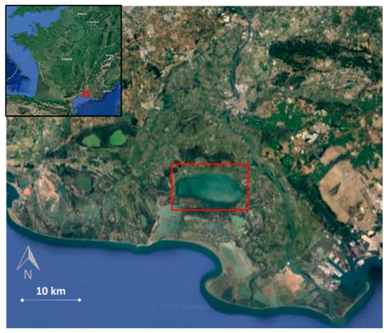
Figure 1.
Study area: lagoon of Vaccarès in the Camargue National Reserve (France).
2.2. Data
2.2.1. Airborne Data
The acquisition of aerial hyperspectral data and water quality measurements (10 stations) were carried out over the study area on 1 July 2019. The aerial hyperspectral images were acquired by Hytech Imaging company at a spatial resolution of 1 m using the HYSPEX sensor flying at an altitude of 2400 m [52]. The sensor records 160 spectral bands in the range of 400–1000 nm with a 3.6 nm bandwidth. The ATCOR algorithm [53] was used to perform the atmospheric correction. Black, grey, and cream-colored ground targets of an area of 5 m2 were positioned to facilitate atmospheric correction. The time slot of the data acquisition was between 11:45 a.m. and 3:45 p.m. Thirty-two flight lines were acquired and merged to obtain a mosaic (Figure 2). Radiometric calibration was carried out for the visible-near infrared data using the manufacturer’s static calibration parameters; in particular, the quantum efficiency, the relative response of the pixel matrix, and spectral calibration were considered. The black current measurement of each image, which was integrated into the raw data headers, was also taken into account. Some of the lines acquired in the north–south direction have been contaminated by the sun glint, which were removed from the raw data as follows. A pixel-by-pixel analysis was carried out to check whether the saturation due to sun glint did not exceed 16 adjacent spectral bands. If not, a spectral interpolation was performed on saturated zones by an Akima-spline interpolator [54]. The pixels exceeding the threshold value of 16 adjacent saturated bands were substituted by the nearest neighbor (among the 4 above, left, right, and bottom) for which the spectral Euclidean distance to the pixel considered on the portion of the unsaturated spectrum was weakest.
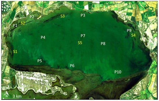
Figure 2.
Red-green-blue (RGB) mosaic measured by HYSPEX airborne instrument. The positions of the in situ sampling stations (stations noted P) and underwater bottom image acquisitions using an in situ camera (stations noted S) are reported.
2.2.2. In Situ Data
Water quality parameter measurements were performed during the flight for 10 sampling stations (Figure 2). Chlorophyll (Chl) concentration data were acquired using the multi-parameter data probe HYDROLAB DS5 equipped with a fluorometric probe. Samples were collected to measure suspended particulate matter (SPM) and colored dissolved organic matter (CDOM). The water samples were acquired at 50 cm beneath the water surface, and they were filtered and weighted to calculate the SPM concentrations [55]. The absorbance was measured in the laboratory using a spectrometer equipped with a double-beam monochromator to calculate the CDOM absorption from an excitation range of 220–600 nm at a 0.2 nm resolution (UV 1800 Shimadzu) [55]. Chlorophyll concentration, suspended particulate matter, and colored dissolved organic matter for each station are given in Table 1.

Table 1.
In situ measurements of water column parameters.
Underwater in situ images were acquired on 17 July 2019 in five stations (Figure 2) across the study area to characterize the benthic diversity and the associated representative spectra of each class of bottom species. Note that the sampling stations used for acquiring these underwater bottom data are not the same as the water quality sampling stations. This is because priority was given to cover the spatial bottom variability of the entire lagoon. The multispectral camera developed by the SILIOS company (http://www.silios.com/multispectral-imaging, accessed on 1 May 2021) was used for the underwater bottom acquisitions (Figure 3). The camera can measure at 8 spectral bands in the visible region, namely 433, 467, 506, 545, 577, 617, 659, and 697 nm, using full-widths at half-maximum of 67, 52, 46, 40, 39, 39, 45, 40, and 9 nm, respectively. The image size is 426 × 339 pixels. The camera was fixed in a waterproof enclosing. More than 300 images were acquired for each station and each image was geo-located using a differential Global Positioning System. The underwater images covered more than 60 m2 for each station. All the images were analyzed using the four bottom classes that were previously defined, namely Sediment, Zosters, Green algae, and Red algae. The Euclidian distance classification method was used based on the training samples within the image. To account for the variation in the illumination caused by the different times of acquisition between each sampling station, the training area was chosen within the images independently for each station. The proportion of each bottom species class within each image was calculated, and the median value over all the images was calculated for each bottom type. The SILIOS images were further used to validate the bottom species composition retrieved from the inversion of satellite data. In parallel to underwater images acquisition, a visual observation using a diving mask was carried out to check the consistency of this approach.
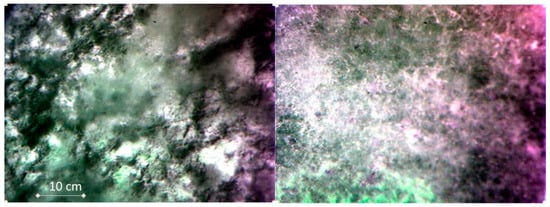
Figure 3.
Examples of bottom composition as measured by the underwater in situ camera developed by the SILIOS company (station S1).
Macrophyte species data have recently been manually collected in the study area and reported by RNNC [50]. The macrophytes data include abundances of overlapping vegetation that was removed by changing the proportion by making them sum to one so that a fair comparison would be possible with the inversion from simulated datasets. The proportion of sediments was also excluded in this comparison because they were not collected by RNNC.
The bottom reflectances for the four benthic classes considered in the study were measured using a portable ASD Handheld-2 device working at a spectral resolution of 1 nm in the range between 350 and 1000 nm. These bottom reflectance spectra were used for the inversion of the semi-analytical model. The reflectance of each bottom class was measured using samples collected by the National Reserve of Camargue staff and brought into the boat deck. The reflectance spectra showed that seagrass and algae-class spectra exhibited a significant increase beyond 700 nm, which is typical of vegetation-like spectra (Figure 4). The spectral shape of Sediment-class reflectance showed an increasing trend with wavelength across the visible range.
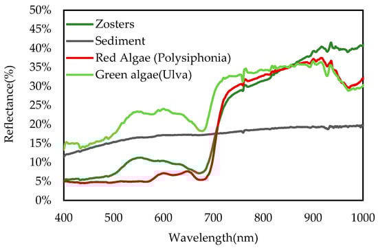
Figure 4.
Spectral variation of the reflectance for each bottom class: Zosters (seagrass), Sediments, and Red and Green algae.
Unfortunately, no Lidar data [56,57] were available on the Camargue site [58]. Bathymetry data were provided by the RNNC. They are based on the merging of data measured over several field campaigns between 1999 and 2013. Due to the shallow depth of the Vaccarès lagoon (average water depth of about 1 m at a water level of 0 m NGF (General Leveling of France)) [58], measurements were carried out using a ruler to determine the water depth, and the corresponding water depth was calculated with a correction of the water level. The raster file of 8 m resolution was obtained by using methods of triangulation and interpolation between the measurements (using the free and open-source cross-platform Qgis, version 3.14.16-Pi). Note that the in situ bathymetry data were acquired at a high time interval in comparison to the airborne data. The order of magnitude of the variations in the bathymetry of the Vaccarès lagoon over several years was studied. The bathymetry measurements performed over the period of 1999–2003 were compared for 281 points with those carried out in 2013. Such a comparison showed that the bathymetry varied by an average of 0.07 m over a 10 to 14 year time period for 281 points of comparison. The variations observed over a decade are thus negligible. Therefore, the comparison of the hyperspectral airborne data acquired in 2019 with the field data used in this study is consistent despite the long time period between the collection of sets of data. To compare the water depth estimated from the images and from the reference bathymetric data, knowledge of the water level is necessary. Measurements were taken from the western and eastern side of the lagoon, every 5 min, and the hourly average was saved. An average of western and eastern measurements was calculated before applying the correction to the whole lagoon [58].
2.2.3. Satellite Sensor Features
The BIODIVERSITY-like sensor will provide a spatial resolution of 8 m and a total of 53 bands between 413 and 990 nm, including 26 bands in the visible range, and a full-width at half-maximum (FWHM) of 10 nm is expected for each band. The targeted signal-to-noise ratio (SNR) was 180 in the visible domain with a revisit time of 5 days. As comparisons of our results were performed with real DESIS data, these sensors are briefly described. The DESIS sensor has a total of 238 bands, including 118 visible bands (between 400 and 700 nm), a spatial resolution of 30 m, an SNR of about 200, and a FWHM of 2.55 nm [17,59].
2.3. Methodology
The overall methodology that was used to simulate a BIODIVERSITY-like image for retrieving water depth and benthic habitat composition is outlined here.
2.3.1. Simulation of Satellite Images from Airborne Hyperspectral Data
The atmospherically corrected hyperspectral airborne data provide the surface water reflectance. Such airborne-derived water reflectance data were used as input of the simulation. The contribution of the atmosphere from the surface level to the satellite level was then added using the MODTRAN radiative transfer model [60] to obtain the top-of-atmosphere radiance. The spatial and spectral resolution of the resulting image was then degraded to match with the satellite sensor’s specifications (BIODIVERSITY), in addition to introducing the noise caused by the sensor itself and inter-band calibration errors. The spectral response function usually used for a hyperspectral sensor is a rectangular function because spectral filters are not employed to decompose the light at various bands, as a diffraction grating is typically used. The spectral bandwidth is so narrow (10 nm) that the spectral response can be modeled satisfactorily using a rectangular function. The simulated satellite image was subsequently corrected for the atmospheric effect to obtain the water reflectance. As the atmospheric correction procedure contained errors, the simulation of the top-of-atmosphere radiance considered two sources of noise. One source of noise was due to the error made on the surface reflectance retrieval (5% at 443 nm), and the other source of noise was due to the error made on the aerosol model. Details of the simulation of the atmospheric correction procedure are given in [61]. This noise was randomly −2% or 2% applied to the simulated spectral reflectance. The water reflectance derived from the satellite simulated data could then be used for deriving the water and bottom parameters. The reader is referred to [15] for details about the methodological aspects of the simulated satellite data. As the calibration error can also lead to an error in the estimation of the water parameters, depth and abundances, a calibration error was added to the simulation processing chain. Usually, a calibration error varies between 0 and 3%. In this study, the inter-band error was fixed at 2% to be realistic based on Centre National Etudes Spatiales (CNES) internal studies [62]
2.3.2. Inversion Method
The semi-analytical model developed by Lee et al. [63] provides the remote sensing surface reflectance (denoted Rrs) as a function of the composition of the water column (chlorophyll concentration—chl, SPM concentration, and CDOM absorption coefficient at 440 nm), and benthic properties (depth—z; abundance of the classes—ai) (Equation (1)). The bottom subsurface reflectance is a linear function of the abundance of each benthic class within the pixel multiplied by the reflectance of each class (measured with the ASD sensor). The sum of abundances is 1.
The inversion of the water reflectance is accomplished by minimizing the Euclidian distance between each pixel of the above-described model (Equation (1)) and the satellite image through optimization. The optimization is driven by a nonlinear curve-fitting in a least-squares sense using the “lsqcurvefit” function in MATLAB with given bounds for each parameter. The inversion results are the optimized values of Chl, SPM, CDOM, and z, and the bottom abundances (ai) of Sediments, Zosters, Green algae, and Red algae for each pixel. When the inversion is achieved, the spatial distributions of the retrieved parameters are then obtained.
2.4. Validation
The parameters estimated from the satellite images were compared with the in situ sampling data as validation. The fractional abundance of the bottom composition was validated using the SILIOS camera underwater images. The performance of the estimation from the satellite data was quantified using the root-mean-square error (RMSE) and relative error (RE). The coefficient of determination (R2) was used to quantify the performance of the estimation of the fractional abundance of different classes estimated from the satellite data in comparison with SILIOS ground-truth data. Finally, the bottom composition retrieved from real hyperspectral images acquired by DESIS was compared with the in situ camera measurements.
The validation was operated using all the available reference values. With regard to bathymetry, the water depths estimated over the entire image were used for comparison with the bathymetric reference data, which were corrected using the water level. The number of values was 1,035,317 at an 8 m resolution and 73,625 values at a 30 m resolution. With regard to the bottom species abundances, 20 reference values were available using the underwater images and 165 reference values were available for the 55 macrophytes stations of validation in the lagoon.
3. Results
The validation of the estimation of water column parameters using the measurement at the 10 in situ measurements provided an RMSE of 1.86 mg.m−3 for the chlorophyll concentration, 3.08 g.m3 for the SPM, and 0.9 m−1 for the CDOM absorption at 440 nm.
3.1. Water Depth Estimates
The water depth retrieved from the simulated BIODIVERSITY-like satellite sensor (Figure 5a) was compared with the bathymetric reference corrected from the water level (Figure 5b). The derived water depth compared well with the in situ data with a high coefficient of determination (slope = 1.18, intercept = 0.36, and R2 = 0.74). The RMSE value that was calculated between the in situ and estimated water depth was 0.28 m, and the RE value was 14.11%. The west–east and north–south spatial transects of the estimated water depth and in situ values exhibited similar behaviors.
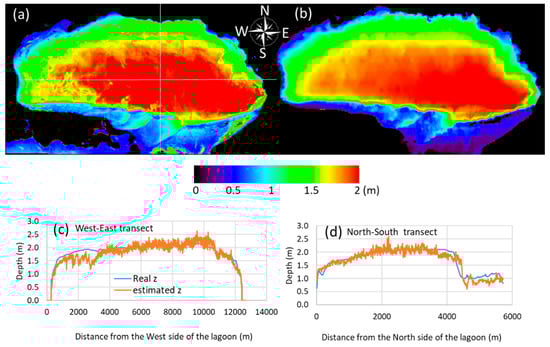
Figure 5.
(a) Retrieved water depth from the simulated BIODIVERSITY datasets; (b) water depth measured in situ using a sounder provided by RNC institute; (c) west–east distribution of water depth along a transect at 43.54° latitude, (d) north–south water depth along a transect at 4.57° longitude. The two transects are identified on Figure 5a by white lines.
As observed in Figure 5, in situ water depth (Figure 5a) showed a similar spatial variation as the derived water depth (Figure 5b). Particularly, the shallower regions in the southern part of the lagoon, as well as in the banks of the lagoon, were consistent. Similarly, the patterns of the relatively deeper regions in the middle of the lagoon were also in agreement with in situ data, although the real data showed smoother variations (Figure 5c,d). A high variability in water depth was visible in the simulated data for the southwestern part of the lagoon, probably due to the fact that the water depth estimation was provided for a better spatial resolution than the bathymetric reference, thus possibly explaining the fact that detailed patterns were noticeable for the retrieval maps, which was not the case when dealing with the water depth reference.
3.2. Bottom Species Composition
The retrieval of the bottom species abundance from the simulated satellite imagery was examined (Figure 6). We should note that their spatial distribution qualitatively matched the visual observations of the patterns of the benthic classes made by the scientific team during the in situ field campaign. It is clear from Figure 6 that the Green algae dominated most of the lagoon while Zosters and Red algae competed for the coastal areas of the lagoon. The presence of the Zosters was also observed on the eastern side of the lagoon. The deeper areas of the lagoon were dominated by the Sediment class.
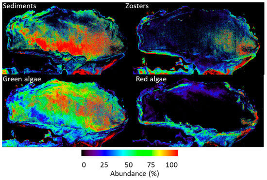
Figure 6.
Retrieval of bottom species class and abundance from the simulated satellite (BIODIVERSITY) data.
The retrieved bottom composition and abundance were also compared with the in situ underwater camera data (Table 2). The inversion method provided the abundance, i.e., the proportion of each class was estimated inside the pixel. Therefore, the 8 m spatial resolution was not limiting, as the mixing was estimated within a given pixel. The method of classification applied to the subaquatic images also provided an abundance within the image; the data were thus not linked to any spatial resolution. The fractional abundance of Sediments derived from the simulated satellite images varied between 0 and 26%, while the same varied between 0 and 16% in underwater camera-based estimations. Similarly, the fractional abundance of Zosters derived from the simulated satellite images varied between 0 and 66%, while the same varied between 0 and 84% in underwater camera-based estimations. For Green algae, the ranges of variation were 0–55% and 0–78%, respectively. For Red algae, the ranges of variation were 19–50% and 8–49%, respectively. A significant correlation between the datasets was observed, as depicted in Figure 7a (R2 value of 0.77).
Table 2.
Comparison of the fractional abundance (in %) of different classes as derived from the simulated images (noted “satellite”) against that obtained from the in situ underwater camera (noted “UW”).
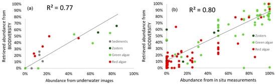
Figure 7.
(a) Comparison of the fractional abundance (in %) of the bottom classes retrieved from the BIODIVERSITY-simulated images with that measured in situ from the underwater images; (b) comparison of the fractional abundance of the macrophytes estimated from the BIODIVERSITY-simulated images with that collected from in situ measurements [50].
The weak abundance of red algae that can be seen in Figure 6 is also visible in Figure 7b. Biodiversity seemed to underestimate its abundance. On the other hand, the high abundance of Green algae that can be seen in Figure 6 was better estimated (Figure 7b). This can be explained by the fact that the higher abundance of Green algae has a higher influence on bottom reflectance than the red algae has, thus being better detected by the sensor and the inversion. It should be highlighted that a significant agreement was observed between measurements of the macrophytes abundance that were measured by SNPN [50] and the inversion from the BIODIVERSITY-like simulated data (R2 value of 0.8, Figure 7b).
4. Discussion
A previous study compared the information provided by the new hyperspectral satellite sensor PRISMA with the multispectral satellite sensor Sentinel-2. The PRISMA TOA radiances were found to be very similar to the Sentinel-2 data, and encouraged the synergic use of both sensors for aquatic applications [34]. Another study examined the potential of PRISMA level 2D images in retrieving standard water quality parameters, including total suspended matter (TSM), chlorophyll-a (Chl-a), and colored dissolved organic matter (CDOM) in a turbid lake (Lake Trasimeno, Italy). The results indicated the high potential of PRISMA level 2D imagery in mapping water quality parameters in Lake Trasimeno. The PRISMA-based retrievals agreed closely with those of Sentinel-2, particularly for TSM [35].
The inversion of the semi-analytical model, which is based on an optimization method relying on a least squares regression, cannot be used with multispectral data, because it requires a high number of spectral bands with regard to the number of parameters that need to be retrieved. In our case, eight parameters had to be estimated, and Sentinel-2 only has 7 spectral bands between 400 and 700 nm, which is not sufficient. Furthermore, the number of spectral bands usually allows the reduction in the impact of the noise on the retrieval. The number of BIODIVERSITY spectral bands (26) allows the reduction in the impact of the noise while the number of Sentinel-2 spectral bands (7) does not permit such a decrease in the noise influence. In addition, the Sentinel-2 and BIODIVERSITY SNR values are 150 and 180 at 450 nm, respectively. The fact that the SNR of BIODIVERSITY is higher than that of Sentinel-2 will lead to a lower influence of the noise on the retrieved parameters.
The present study showed that the future BIODIVERSITY sensor will be able to estimate the water depth comparable with an RMSE of 0.28 m, RE value of 14.11%, and consistent benthic fractional abundance (0.77 with underwater images and 0.8 with measurements of the macrophytes abundance that were measured by SNPN).
To compare the estimation of the bio-optical parameters retrieved from BIODIVERSITY simulations with those retrieved from real hyperspectral satellite images, the inversion methodology was applied to DESIS real data for the same location. Two DESIS images were processed. One was acquired on 4 September 2019 and the other was acquired on 2 February 2020. The first image was the closest in time with the BIODIVERSITY simulation and in situ measurements; however, the lagoon area was not entirely covered by the DESIS sensor. As benthic habitats show a seasonal cycle, the image acquired on 4 September 2019 was preferred to compare with in situ benthic reference (Figure 8. The second DESIS image (which was acquired on 2 February 2020) covers the entire lagoon area. This image was selected to compare with the water depth reference (Figure 9).
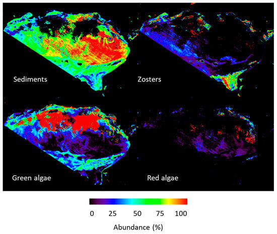
Figure 8.
Retrieval of benthic composition from DESIS data (4 September 2019).
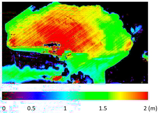
Figure 9.
Inversion of DESIS data to retrieve water depth using Lee’s method. The DESIS satellite image was acquired on 1 February 2020.
The water depth validation was operated using the bathymetric reference corrected from the water level. The raster file was resized for comparison with the water depth obtained from DESIS (30 m resolution). Such a resizing was operated using a 3.75x3.75-pixel window followed by a downsampling in order to obtain a 30 m resolution raster file. The water depth patterns were observed to be different from those observed using either the BIODIVERSITY-like sensor (Figure 5a) or the in situ ground truth data (Figure 5b). This is likely due to the lower spatial resolution of the DESIS sensor (30 m) in contrast to the BIODIVERSITY-like sensor (8 m). Black pixels in the southern part of the DESIS scene were not processed, because they were covered by a very small cloud.
The RMSE between the DESIS-derived water depth and the in situ water depth was 0.38 m, and the RE was 17%. The BIODIVERSITY-like sensor-retrieved water depth (Figure 5) was observed to have a lower RMSE (0.28 m) and RE (14.11%) than those of the DESIS retrieval, thus revealing the great interest and potential of a satellite sensor, showing similar features as the BIODIVERSITY sensor.
Figure 9 shows the retrieval of the benthic composition from DESIS data using Lee’s method. The Sediment class was the most dominant class (>60%) over the entire area. A high amount of Green algae (>90%) was retrieved in the north of the Lagoon and a negligible amount of Zoster and Red algae was observed (<10%). The composition of Green algae and Sediment highly contrasted with the results derived from BIODIVERSITY inversion, which showed a much higher abundance of Green algae over the Lagoon. A patch of Zosters was observed close to the banks in the southeast side of the lagoon from the retrieval. Such patches of Zosters could also be observed from the BIODIVERSITY retrieval for the same area, although the spatial pattern differed slightly. The statistics of the comparison between the DESIS-retrieved bottom composition with the in situ macrophyte data [50] are shown. An R2 value of 0.68 was obtained. However, the same comparison made using the BIODIVERSITY-like simulated image yielded an R2 value of 0.80 (Figure 7), which highlights again the advantage of using a BIODIVERSITY-like sensor for the benthic habitat mapping in inland shallow waters. Besides, a high standard deviation was obtained for the DESIS-derived macrophyte data in comparison with the in situ measurements, which was lower in the case of the BIODIVERSITY-like simulated image (Figure 7).
In Figure 10, it seems that the retrieval of the fractional abundance from DESIS data yielded a higher number of samples that were classified either as 0% or 100% for a given class as compared to BIODIVERSITY data. This indicates a systematic misclassification due to the low spatial resolution of DESIS (30 m) compared with the BIODIVERSITY resolution (8 m). Red algae, which were in weak abundance, were not properly captured by the inversion of DESIS data. On the other hand, Green algae, which were in high abundance, were overestimated by the inversion of DESIS data. Compared to the validation operated with the BIODIVERSTIY sensor (Figure 7b), the abundances of these two classes were better estimated using the BIODIVERSITY sensor. This was probably due to the higher resolution of BIODIVERSITY compared to DESIS.
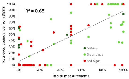
Figure 10.
Overall comparison of DESIS estimates of the fraction abundance (in percentage) of benthic composition with in situ data [50].
This study was carried out for an inland area; however, it should be noted that our results cannot be generalized to all inland waters. For example, in the current study, the waters were very shallow (<2 m), which allows the depth and benthic abundance to be satisfactorily estimated. The retrievals would probably be less for darker waters. Finally, the summertime period was selected for acquiring the data to optimize the detection of the benthic habitat.
5. Conclusions
The investigation of the benthic properties of shallow inland waters based on the hyperspectral remote sensing technique using a sensor such as BIODIVERSITY is relevant for retrieving benthic habitat composition and water depth. Here, the atmospheric and sensor noise effects were considered to invert the satellite-level data obtained from aerial measurements. A semi-analytical approach coupled with optimization techniques was used for that purpose. It was shown that the estimation of water depth was satisfactory (RMSE = 0.28 m and RE = 14.11%). Similarly, the significant agreement of the derived benthic habitat composition with in situ observations, typically R2 = 0.77, based on the comparison with the underwater camera, the estimated benthic composition, and R2 = 0.8, based on the comparison with the RNNC collected in situ macrophytes data, points out the high potential of the spectral (53 bands and 10 nm spectral resolution) and spatial (8 m) characteristics of a BIODIVERSITY-like sensor for characterizing shallow inland waters. It was demonstrated that the BIODIVERSITY-like sensor configuration will be beneficial in comparison with existing sensors like DESIS for estimating the water depth and for mapping the benthic habitats. The spatial resolution of 30 m that characterizes the DESIS sensor is likely to be too coarse to lead to a better retrieval of the water depth (RMSE = 0.38 m and RE = 17%) and bottom composition (R2 = 0.68) in shallow inland waters such as the Vaccarès lagoon in comparison with the BIODIVERSITY-like sensor configuration. In this study, classes with high abundances such as Green algae were overestimated using DESIS, and classes with weak abundances such as Red algae were underestimated; this is probably due to the coarser resolution compared to BIODIVERSITY. Other studies could be carried out in darker and deeper lakes or in different seasons to test the robustness of the method.
Author Contributions
Conceptualization, A.M., M.C. and M.G.; methodology, A.M., M.C. and M.G.; software, A.M. and S.V.-C.; validation, E.M., P.G. and O.B.; formal analysis, A.M., M.C. and M.G.; investigation, A.M., M.C. and M.G.; resources, A.M., M.C. and M.G.; data curation, S.V.-C. and O.B.; writing—original draft preparation, S.V.-C.; writing—review and editing, A.M., M.C., M.G., O.B., E.M. and P.G.; visualization, S.V.-C.; supervision, A.M.; project administration, A.M.; funding acquisition, A.M., M.C. and M.G. All authors have read and agreed to the published version of the manuscript.
Funding
This work was financially supported by TOSCA-CNES, France.
Institutional Review Board Statement
Not applicable.
Informed Consent Statement
Not applicable.
Acknowledgments
The authors are thankful to Uta Heiden and Nicole Pinnel from DLR (Germany) for providing DESIS data. They are also grateful to Stéphane Tisserand and Aurélien Faiola from SILIOS Technologies SA, France, for providing the underwater camera and for performing the data acquisition.
Conflicts of Interest
The authors declare no conflict of interest.
References
- Vahtmäe, E.; Paavel, B.; Kutser, T. How much benthic information can be retrieved with hyperspectral sensor from the optically complex coastal waters? J. Appl. Remote Sens. 2020, 14, 016504. [Google Scholar] [CrossRef]
- Alevizos, E. A Combined Machine Learning and Residual Analysis Approach for Improved Retrieval of Shallow Bathymetry from Hyperspectral Imagery and Sparse Ground Truth Data. Remote Sens. 2020, 12, 3489. [Google Scholar] [CrossRef]
- Pérez-Ruzafa, A.; Marcos, C.; Pérez-Ruzafa, I. Mediterranean coastal lagoons in an ecosystem and aquatic resources management context. Phys. Chem. Earth Parts A/B/C 2011, 36, 160–166. [Google Scholar] [CrossRef]
- Le Fur, I.; De Wit, R.; Plus, M.; Oheix, J.; Simier, M.; Ouisse, V. Submerged benthic macrophytes in Mediterranean lagoons: Distribution patterns in relation to water chemistry and depth. Hydrobiologia 2017, 808, 175–200. [Google Scholar] [CrossRef]
- Zaldívar, J.-M.; Viaroli, P.; Newton, A.; De Wit, R.; Ibañez, C.; Reizopoulou, S.; Somma, F.; Razinkovas, A.; Basset, A.; Holmer, M.; et al. Eutrophication in Transitional Waters: An Overview. Transit. Waters Monogr. 2008, 2, 1–78. [Google Scholar]
- Toso, C.; Madricardo, F.; Molinaroli, E.; Fogarin, S.; Kruss, A.; Petrizzo, A.; Pizzeghello, N.M.; Sinapi, L.; Trincardi, F. Tidal inlet seafloor changes induced by recently built hard structures. PLoS ONE 2019, 14, e0223240. [Google Scholar] [CrossRef]
- Janowski, L.; Madricardo, F.; Fogarin, S.; Kruss, A.; Molinaroli, E.; Kubowicz-Grajewska, A.; Tegowski, J. Spatial and Temporal Changes of Tidal Inlet Using Object-Based Image Analysis of Multibeam Echosounder Measurements: A Case from the Lagoon of Venice, Italy. Remote Sens. 2020, 12, 2117. [Google Scholar] [CrossRef]
- Guelorget, O.; Frisoni, G.; Perthuisot, J. La Zonation Biologique Des Milieux Lagunaires: Définition d’une Échelle de Confinement Dans Le Domaine Paralique Méditerranéen. J. Rech. Oceanogr. 1983, 8, 15–35. [Google Scholar]
- Sarà, G.; Leonardi, M.; Mazzola, A. Spatial and Temporal Changes of Suspended Matter in Relation to Wind and Vegetation Cover in A Mediterranean Shallow Coastal Environment. Chem. Ecol. 1999, 16, 151–173. [Google Scholar] [CrossRef]
- Millet, B.; Guelorget, O. Spatial and seasonal variability in the relationships between benthic communities and physical environment in a lagoon ecosystem. Mar. Ecol. Prog. Ser. 1994, 108, 161–174. [Google Scholar] [CrossRef]
- Bachelet, G.; De Montaudouin, X.; Auby, I.; Labourg, P.-J. Seasonal changes in macrophyte and macrozoobenthos assemblages in three coastal lagoons under varying degrees of eutrophication. ICES J. Mar. Sci. 2000, 57, 1495–1506. [Google Scholar] [CrossRef]
- Viaroli, P.; Bartoli, M.; Giordani, G.; Naldi, M.; Orfanidis, S.; Zaldivar, J.M. Community shifts, alternative stable states, biogeochemical controls and feedbacks in eutrophic coastal lagoons: A brief overview. Aquat. Conserv. Mar. Freshw. Ecosyst. 2008, 18, S105–S117. [Google Scholar] [CrossRef]
- Souchu, P.; Bec, B.; Smith, V.H.; Laugier, T.; Fiandrino, A.; Benau, L.; Orsoni, V.; Collos, Y.; Vaquer, A. Patterns in nutrient limitation and chlorophyll a along an anthropogenic eutrophication gradient in French Mediterranean coastal lagoons. Can. J. Fish. Aquat. Sci. 2010, 67, 743–753. [Google Scholar] [CrossRef]
- Casey, B.; Lee, Z.; Arnone, R.A.; Weidemann, A.D.; Parsons, R.; Montes, M.J.; Gao, B.-C.; Goode, W.; Davis, C.O.; Dye, J. Water and bottom properties of a coastal environment derived from Hyperion data measured from the EO-1 spacecraft platform. J. Appl. Remote Sens. 2007, 1, 011502. [Google Scholar] [CrossRef]
- Minghelli, A.; Vadakke-Chanat, S.; Chami, M.; Guillaume, M.; Peirache, M. Benefit of the Potential Future Hyperspectral Satellite Sensor (BIODIVERSITY) for Improving the Determination of Water Column and Seabed Features in Coastal Zones. IEEE J. Sel. Top. Appl. Earth Obs. Remote Sens. 2021, 14, 1222–1232. [Google Scholar] [CrossRef]
- Zhang, C. Applying data fusion techniques for benthic habitat mapping and monitoring in a coral reef ecosystem. ISPRS J. Photogramm. Remote Sens. 2015, 104, 213–223. [Google Scholar] [CrossRef]
- Alonso, K.; Bachmann, M.; Burch, K.; Carmona, E.; Cerra, D.; Reyes, R.D.L.; Dietrich, D.; Heiden, U.; Hölderlin, A.; Ickes, J.; et al. Data Products, Quality and Validation of the DLR Earth Sensing Imaging Spectrometer (DESIS). Sensors 2019, 19, 4471. [Google Scholar] [CrossRef]
- Cho, H.J.; Ogashawara, I.; Mishra, D.; White, J.; Kamerosky, A.; Morris, L.; Clarke, C.; Simpson, A.; Banisakher, D. Evaluating Hyperspectral Imager for the Coastal Ocean (HICO) data for seagrass mapping in Indian River Lagoon, FL. GIScience Remote Sens. 2014, 51, 120–138. [Google Scholar] [CrossRef]
- Garcia, R.A.; McKinna, L.I.; Hedley, J.D.; Fearns, P.R. Improving the optimization solution for a semi-analytical shallow water inversion model in the presence of spectrally correlated noise. Limnol. Oceanogr. Methods 2014, 12, 651–669. [Google Scholar] [CrossRef]
- Giardino, C.; Bresciani, M.; Cazzaniga, I.; Schenk, K.; Rieger, P.; Braga, F.; Matta, E.; Brando, V.E. Evaluation of Multi-Resolution Satellite Sensors for Assessing Water Quality and Bottom Depth of Lake Garda. Sensors 2014, 14, 24116–24131. [Google Scholar] [CrossRef]
- Hedley, J.D.; Russell, B.J.; Randolph, K.; Pérez-Castro, M.Á.; Vásquez-Elizondo, R.M.; Enríquez, S.; Dierssen, H.M. Remote Sensing of Seagrass Leaf Area Index and Species: The Capability of a Model Inversion Method Assessed by Sensitivity Analysis and Hyperspectral Data of Florida Bay. Front. Mar. Sci. 2017, 4. [Google Scholar] [CrossRef]
- Meerdink, S.K.; Roberts, D.A.; Roth, K.L.; King, J.Y.; Gader, P.D.; Koltunov, A. Classifying California plant species temporally using airborne hyperspectral imagery. Remote Sens. Environ. 2019, 232, 111308. [Google Scholar] [CrossRef]
- Giardino, C.; Brando, V.E.; Gege, P.; Pinnel, N.; Hochberg, E.; Knaeps, E.; Reusen, I.; Doerffer, R.; Bresciani, M.; Braga, F.; et al. Imaging Spectrometry of Inland and Coastal Waters: State of the Art, Achievements and Perspectives. Surv. Geophys. 2019, 40, 401–429. [Google Scholar] [CrossRef]
- Khan, M.J.; Khan, H.S.; Yousaf, A.; Khurshid, K.; Abbas, A. Modern Trends in Hyperspectral Image Analysis: A Review. IEEE Access 2018, 6, 14118–14129. [Google Scholar] [CrossRef]
- Jay, S.; Guillaume, M.; Minghelli, A.; Deville, Y.; Chami, M.; Lafrance, B.; Serfaty, V. Hyperspectral remote sensing of shallow waters: Considering environmental noise and bottom intra-class variability for modeling and inversion of water reflectance. Remote Sens. Environ. 2017, 200, 352–367. [Google Scholar] [CrossRef]
- Lee, Z.; Carder, K.L. Effect of spectral band numbers on the retrieval of water column and bottom properties from ocean color data. Appl. Opt. 2002, 41, 2191–2201. [Google Scholar] [CrossRef] [PubMed]
- Kerr, G.; Avbelj, J.; Carmona, E.; Eckardt, A.; Gerasch, B.; Graham, L.; Gunther, B.; Heiden, U.; Krutz, D.; Krawczyk, H.; et al. The hyperspectral sensor DESIS on MUSES: Processing and applications. IEEE Int. Geosci. Remote Sens. Symp. IGARSS 2016, 2016, 268–271. [Google Scholar] [CrossRef]
- Loizzo, R.; Guarini, R.; Longo, F.; Scopa, T.; Formaro, R.; Facchinetti, C.; Varacalli, G. Prisma: The Italian Hyperspectral Mission. In Proceedings of the IGARSS 2018 IEEE International Geoscience and Remote Sensing Symposium, Valencia, Spain, 22–27 July 2018; pp. 175–178. [Google Scholar]
- Liu, Y.-N.; Zhang, J.; Sun, W.-W.; Jiao, L.-L.; Sun, D.-X.; Hu, X.-N.; Ye, X.; Li, Y.-D.; Liu, S.-F.; Cao, K.-Q.; et al. The Advanced Hyperspectral Imager: Aboard China’s GaoFen-5 Satellite. IEEE Geosci. Remote Sens. Mag. 2019, 7, 23–32. [Google Scholar] [CrossRef]
- Mahalingam, S.; Srinivas, P.; Devi, P.K.; Sita, D.; Das, S.K.; Leela, T.S.; Venkataraman, V.R. Reflectance based vicarious calibration of HySIS sensors and spectral stability study over pseudo-invariant sites. In Proceedings of the 2019 IEEE Recent Advances in Geoscience and Remote Sensing: Technologies, Standards and Applications (TENGARSS), Kochi, India, 17–20 October 2019; pp. 132–136. [Google Scholar]
- Palmer, S.C.; Kutser, T.; Hunter, P.D. Remote sensing of inland waters: Challenges, progress and future directions. Remote Sens. Environ. 2015, 157, 1–8. [Google Scholar] [CrossRef]
- Banerjee, S.; Shanmugam, P. Novel method for reconstruction of hyperspectral resolution images from multispectral data for complex coastal and inland waters. Adv. Space Res. 2021, 67, 266–289. [Google Scholar] [CrossRef]
- Topp, S.N.; Pavelsky, T.M.; Jensen, D.; Simard, M.; Ross, M.R.V. Research Trends in the Use of Remote Sensing for Inland Water Quality Science: Moving Towards Multidisciplinary Applications. Water 2020, 12, 169. [Google Scholar] [CrossRef]
- Giardino, C.; Bresciani, M.; Braga, F.; Fabbretto, A.; Ghirardi, N.; Pepe, M.; Gianinetto, M.; Colombo, R.; Cogliati, S.; Ghebrehiwot, S.; et al. First Evaluation of PRISMA Level 1 Data for Water Applications. Sensors 2020, 20, 4553. [Google Scholar] [CrossRef] [PubMed]
- Niroumand-Jadidi, M.; Bovolo, F.; Bruzzone, L. Water Quality Retrieval from PRISMA Hyperspectral Images: First Experience in a Turbid Lake and Comparison with Sentinel-2. Remote Sens. 2020, 12, 3984. [Google Scholar] [CrossRef]
- Mobley, C.D. Light and Water: Radiative Transfer in Natural Waters; Academic Press: San Diego, CA, USA, 1994. [Google Scholar]
- Petit, T.; Bajjouk, T.; Mouquet, P.; Rochette, S.; Vozel, B.; Delacourt, C. Hyperspectral remote sensing of coral reefs by semi-analytical model inversion–Comparison of different inversion setups. Remote Sens. Environ. 2017, 190, 348–365. [Google Scholar] [CrossRef]
- Muzirafuti, A.; Barreca, G.; Crupi, A.; Faina, G.; Paltrinieri, D.; Lanza, S.; Randazzo, G. The Contribution of Multispectral Satellite Image to Shallow Water Bathymetry Mapping on the Coast of Misano Adriatico, Italy. J. Mar. Sci. Eng. 2020, 8, 126. [Google Scholar] [CrossRef]
- Niroumand-Jadidi, M.; Vitti, A.; Lyzenga, D.R. Multiple Optimal Depth Predictors Analysis (MODPA) for river bathymetry: Findings from spectroradiometry, simulations, and satellite imagery. Remote Sens. Environ. 2018, 218, 132–147. [Google Scholar] [CrossRef]
- Niroumand-Jadidi, M.; Bovolo, F.; Bruzzone, L. SMART-SDB: Sample-specific multiple band ratio technique for satellite-derived bathymetry. Remote Sens. Environ. 2020, 251, 112091. [Google Scholar] [CrossRef]
- Minghelli-Roman, A.; Dupouy, C. Correction of the Water Column Attenuation: Application to the Seabed Mapping of the Lagoon of New Caledonia Using MERIS Images. IEEE J. Sel. Top. Appl. Earth Obs. Remote Sens. 2014, 7, 2619–2629. [Google Scholar] [CrossRef]
- Minghelli-Roman, A.; Polidori, L.; Mathieu, S.; Loubersac, L.; Cauneau, F. Bathymetric Estimation Using MERIS Images in Coastal Sea Waters. IEEE Geosci. Remote Sens. Lett. 2007, 4, 274–277. [Google Scholar] [CrossRef][Green Version]
- Minghelli-Roman, A.; Goreac, A.; Mathieu, S.; Spigai, M.; Gouton, P. Comparison of bathymetric estimation using different satellite images in coastal sea waters. Int. J. Remote Sens. 2009, 30, 5737–5750. [Google Scholar] [CrossRef]
- Dekker, A.G.; Phinn, S.; Anstee, J.M.; Bissett, P.; Brando, V.E.; Casey, B.; Fearns, P.; Hedley, J.; Klonowski, W.; Lee, Z.P.; et al. Intercomparison of shallow water bathymetry, hydro-optics, and benthos mapping techniques in Australian and Caribbean coastal environments. Limnol. Oceanogr. Methods 2011, 9, 396–425. [Google Scholar] [CrossRef]
- Lee, Z.; Carder, K.L.; Mobley, C.D.; Steward, R.G.; Patch, J.S. Hyperspectral remote sensing for shallow waters I A semianalytical model. Appl. Opt. 1998, 37, 6329–6338. [Google Scholar] [CrossRef] [PubMed]
- Brando, V.E.; Anstee, J.M.; Wettle, M.; Dekker, A.G.; Phinn, S.; Roelfsema, C. A physics based retrieval and quality assessment of bathymetry from suboptimal hyperspectral data. Remote Sens. Environ. 2009, 113, 755–770. [Google Scholar] [CrossRef]
- Jay, S.; Guillaume, M. A novel maximum likelihood based method for mapping depth and water quality from hyperspectral remote-sensing data. Remote Sens. Environ. 2014, 147, 121–132. [Google Scholar] [CrossRef]
- Chauvelon, P. A wetland managed for agriculture as an interface between the Rhône river and the Vaccarès lagoon (Camargue, France): Transfers of water and nutrients. Hydrobiologia 1998, 373/374, 181–191. [Google Scholar] [CrossRef]
- Millet, B.; Robert, C.; Grillas, P.; Coughlan, C.; Banas, D. Numerical modelling of vertical suspended solids concentrations and irradiance in a turbid shallow system (Vaccares, Se France). Hydrobiologia 2009, 638, 161–179. [Google Scholar] [CrossRef]
- Espel, D.; Diepens, N.J.; Boutron, O.; Buffan-Dubau, E.; Chérain, Y.; Coulet, E.; Grillas, P.; Probst, A.; Silvestre, J.; Elger, A. Dynamics of the seagrass Zostera noltei in a shallow Mediterranean lagoon exposed to chemical contamination and other stressors. Estuarine Coast. Shelf Sci. 2019, 222, 1–12. [Google Scholar] [CrossRef]
- Vaquer, A.; Heurteaux, P. Modifications Récentes de La Végétation Aquatique de l’étang Du Vaccarès (Camargue, France) Liées Aux Perturbations Anthropiques. In Proceedings of the Annales de Limnologie, Camargue, France, 15 August 2009; Volume 25, pp. 25–38. [Google Scholar]
- Köhler, C.H. Airborne Imaging Spectrometer HySpex. J. Large-Scale Res. Facil. JLSRF 2016, 2, 93. [Google Scholar] [CrossRef]
- Richter, R.; Schläpfer, D. Atmospheric/Topographic Correction for Satellite Imagery (ATCOR-2/3 User Guide, Version 8.2 BETA, February 2012) ATCOR-2/3 User Guide, Version 8.2.0; ReSe Applications Schläpfer: Wil, Switzerland, 2013. [Google Scholar]
- Wang, Y.; Yang, D.; Liu, Y. A real-time look-ahead interpolation algorithm based on Akima curve fitting. Int. J. Mach. Tools Manuf. 2014, 85, 122–130. [Google Scholar] [CrossRef]
- Mueller, J.L.; Fargion, G.S.; Mcclain, C.R.; Clark, D.K.; Kuwahara, V.S.; Lazin, G.; Brown, S.W.; Yarbrough, M.A.; Feinholz, M.; Flora, S.; et al. Special Topics in Ocean Optics Protocols and Appendices. In Ocean Optics Protocols for Satellite Ocean Color Sensor Validation; Revision 4; Goddard Space Flight Space Center: Greenbelt, MD, USA, 2003; Volume VI. [Google Scholar]
- Agrafiotis, P.; Karantzalos, K.; Georgopoulos, A.; Skarlatos, D. Correcting Image Refraction: Towards Accurate Aerial Image-Based Bathymetry Mapping in Shallow Waters. Remote Sens. 2020, 12, 322. [Google Scholar] [CrossRef]
- Costa, B.; Battista, T.; Pittman, S. Comparative evaluation of airborne LiDAR and ship-based multibeam SoNAR bathymetry and intensity for mapping coral reef ecosystems. Remote Sens. Environ. 2009, 113, 1082–1100. [Google Scholar] [CrossRef]
- Boutron, O.; Bertrand, O.; Fiandrino, A.; Höhener, P.; Sandoz, A.; Chérain, Y.; Coulet, E.; Chauvelon, P. An Unstructured Numerical Model to Study Wind-Driven Circulation Patterns in a Managed Coastal Mediterranean Wetland: The Vaccarès Lagoon System. Water 2015, 7, 5986–6016. [Google Scholar] [CrossRef]
- Krutz, D.; Müller, R.; Knodt, U.; Günther, B.; Walter, I.; Sebastian, I.; Säuberlich, T.; Reulke, R.; Carmona, E.; Eckardt, A.; et al. The Instrument Design of the DLR Earth Sensing Imaging Spectrometer (DESIS). Sensors 2019, 19, 1622. [Google Scholar] [CrossRef] [PubMed]
- Boudouresque, C.F.; Bernard, G.; Pergent, G.; Shili, A.; Verlaque, M. Regression of Mediterranean seagrasses caused by natural processes and anthropogenic disturbances and stress: A critical review. Bot. Mar. 2009, 52. [Google Scholar] [CrossRef]
- Gross, L.; Thiria, S.; Mitchell, B.G.; Frouin, R. Artificial neural networks for modeling the transfer function between marine reflectance and phytoplankton pigment concentration. J. Geophys. Res. Space Phys. 2000, 105, 3483–3495. [Google Scholar] [CrossRef]
- Lennon, M.; Jamet, C. Évaluation de l’effet Des Corrections Atmosphériques et Des Caractéristiques Instrumentales d’une Mission Hyperspectrale Pour La Couleur de l’eau En Milieu Côtier; Internal CNES Report; CNES: Toulouse, France, 2020.
- Lee, Z.; Carder, K.L.; Mobley, C.D.; Steward, R.G.; Patch, J.S. Hyperspectral remote sensing for shallow waters: 2 Deriving bottom depths and water properties by optimization. Appl. Opt. 1999, 38, 3831–3843. [Google Scholar] [CrossRef]
Publisher’s Note: MDPI stays neutral with regard to jurisdictional claims in published maps and institutional affiliations. |
© 2021 by the authors. Licensee MDPI, Basel, Switzerland. This article is an open access article distributed under the terms and conditions of the Creative Commons Attribution (CC BY) license (https://creativecommons.org/licenses/by/4.0/).