Article

Rich CNN Features for Water-Body Segmentation from Very High Resolution Aerial and Satellite Imagery

1
School of Remote Sensing and Information Engineering, Wuhan University, Wuhan 430079, China
2
Department of Physical Geography, Utrecht University, 3584 CB Utrecht, The Netherlands
3
Zhejiang Academy of Surveying and Mapping, Hangzhou 310023, China
*
Author to whom correspondence should be addressed.
Remote Sens. 2021, 13(10), 1912; https://doi.org/10.3390/rs13101912
Submission received: 22 March 2021 / Revised: 29 April 2021 / Accepted: 9 May 2021 / Published: 13 May 2021

Abstract

:
Extracting water-bodies accurately is a great challenge from very high resolution (VHR) remote sensing imagery. The boundaries of a water body are commonly hard to identify due to the complex spectral mixtures caused by aquatic vegetation, distinct lake/river colors, silts near the bank, shadows from the surrounding tall plants, and so on. The diversity and semantic information of features need to be increased for a better extraction of water-bodies from VHR remote sensing images. In this paper, we address these problems by designing a novel multi-feature extraction and combination module. This module consists of three feature extraction sub-modules based on spatial and channel correlations in feature maps at each scale, which extract the complete target information from the local space, larger space, and between-channel relationship to achieve a rich feature representation. Simultaneously, to better predict the fine contours of water-bodies, we adopt a multi-scale prediction fusion module. Besides, to solve the semantic inconsistency of feature fusion between the encoding stage and the decoding stage, we apply an encoder-decoder semantic feature fusion module to promote fusion effects. We carry out extensive experiments in VHR aerial and satellite imagery respectively. The result shows that our method achieves state-of-the-art segmentation performance, surpassing the classic and recent methods. Moreover, our proposed method is robust in challenging water-body extraction scenarios.

Graphical Abstract

1. Introduction

Water-body extraction is of great significance in water resources monitoring, natural disaster assessment and environmental protection [1,2,3]. These applications rely on the quantification of the water-body change. Accurately obtaining water-body segmentation from remote sensing images is an important mission for monitoring water body changes. In this paper, our aim is to accurately delineate water-bodies in complicated and challenging scenarios from very high resolution (VHR) remote sensing imagery. Instruments onboard satellites and aerial vehicles provide remote sensing imagery that covers large-scale water surface on Earth. As shown in Figure 1, the contours of water-body in VHR remote sensing images are often unclear. Such degradations are typically caused by aquatic vegetation blocking, silts/boats near the bank and shadows from the surrounding tall plants. The distinct colors are commonly caused by imaging conditions, water quality and microorganisms. Hence, it is a great challenge to extract the outline of water-bodies accurately in complex scenes from VHR remote sensing imagery.
Traditionally, the existing methods of extracting water-bodies from remote sensing images mainly focus on the spectral characteristics of each band and the manually designed features, such as band threshold-based methods [4], supervised classification-based methods [5], water and vegetation indices-based methods [6], and spectral relationship-based methods [7]. However, these methods pay little attention to the spatial information (i.e., shape, size, texture, edge, shadow, and context semantics) of the water-bodies, which significantly affects the classification accuracy. For massive remote sensing images, the drawbacks of traditional methods additionally include their low degree of automation.
Convolutional neural network (CNN) has shown remarkable performance in image classification, target detection and semantic segmentation [8,9,10,11,12,13], creditable to the strong feature representation ability of CNN. Long et al. [8] first proposed the fully convolutional network (FCN), which replaces the last fully connected layers with convolutional ones to achieve end-to-end semantic segmentation. Hereafter, FCNs in an end-to-end manner are widely applied and extensively developed, becoming a mainstream technology in semantic segmentation and edge detection [12,13,14,15,16,17,18]. Ronneberger et al. [9] designed a contracting path and a symmetric expanding path to merge different semantic features for biomedical image segmentation. Lin et al. [10] made full use of the feature information available in the down-sampling process and used long-distance residual connections to achieve high-resolution prediction. Yu et al. [11] proposed an end-to-end deep semantic edge learning architecture for category-aware semantic edge detection. Bertasius et al. [12] presented a multi-scale bifurcated deep network, which exploited object-related features as high-level cues for contour detection. Xie et al. [13] developed a novel convolutional neural-network-based edge detection system by combining multi-scale and multi-level visual responses.
Recently, deep learning-based water-body segmentation from remote sensing imagery has attracted some attention and developments [14,15,16,17,18]. Yu et al. [14] pioneers at introducing a CNN-based method for water-body extraction from Landsat imagery by considering both spectral and spatial information. However, this CNN-based method cut an image into small tiles for pixel-level predictions, which introduced a lot of redundancy and is of low efficiency. Miao et al. [15] proposed a restricted receptive field deconvolution network to extract water bodies from high-resolution remote sensing images. Li et al. [16] adopted a typical FCN model to extract water bodies from VHR images and significantly outperformed the normalized difference water index (NDWI) based method, the support vector machine (SVM) based method, and the sparsity model (SM) based method. However, these two approaches didn’t consider the multi-scale information from different decoder layers and the channel relationship of feature maps in the encoder, which incorporated insufficient extraction of water bodies in complex scenes. Duan et al. [17] proposed a novel multi-scale refinement network (MSR-Net) for water-body segmentation, which made full use of the multi-scale features for more accurate segmentation. However, the MSR-Net does not reuse high-level semantic information and the multi-scale module it possesses does not consider channel relationships between feature maps. Guo et al. [18] adopted a simple FCN-based method for water-body extraction and presented a multi-scale feature extractor, including four dilated convolutions with different rates, which was deployed on top of the encoders. This FCN-based method simply used the multi-scale information of high-level semantic features, but did not extract complete features at other scales. It is evident that current FCN-based water extraction studies emphasized feature extraction and prediction optimization, but the room for further improvements is considerable. Feature fusion in the FCN-based method preferably combines high-semantic features and features with precise locations, which facilitates water-body identification and the accurate extraction of water-body edges. In this work, we design our method by considering three aspects: feature extraction, prediction optimization, and the feature fusion of shallow and deep layers.
How to design optimal multi-layer convolution structures to extract excellent features from images has been widely studied in visual tasks. Simonyan and Zisserman [19] stacked deep convolutional layers to enhance the feature representation, which has been proven to be effective in large-scale image classification. He et al. [20] presented a residual learning framework to further deepen networks to achieve better feature representation ability. Huang et al. [21] established dense connections between the front layers and the back layers to promote the reuse of features. These methods mainly utilize the convolution operation itself to learn layer-wise local feature representations and use pooling operations to expand the receptive field. However, between-layer and local-global feature representation ability may require to be further improved. Zhang et al. [22] proposed a split-attention module to focus on the relationship between different feature groups to achieve better feature extraction results. However, this approach mainly considered local information and the between-channel relationship of the feature maps at each scale, but neglected larger receptive fields information of feature maps. To fully extract water-body features in complex scenes from VHR remote sensing imagery, we design a multi-feature extraction and combination module to extract rich features from both small and large receptive fields and between-channel information to increase the feature representation ability.
Prediction optimization: To obtain more refined semantic segmentation results, especially better edges and boundaries, many researchers optimize the rough prediction results [10,23,24,25]. Lin et al. [10] used long-distance residual connections for all multi-scale features in the down-sampling process to achieve high-resolution prediction. Qin et al. [23] designed an independent encoder-decoder, named residual refine module (RRM), to post-process the semantic segmentation results. Yu et al. [24] proposed the refinement residual block (RRB) to optimize the feature maps. Cheng et al. [25] designed a special-purpose refine network via global and local refinement to optimize the rough prediction results. However, most of these methods may introduce redundancy due to the repeated structural design. In our method, based on the features extracted from our feature extraction module, we propose a simple and effective multi-scale prediction optimization module to refine the water-body predictions from different scales.
Feature fusion: In semantic segmentation, shallow features have accurate localization while deep features consist advanced semantic information. The fusion of deep and shallow features plays an important role in achieving high-precision semantic segmentation [9,26,27,28]. Ronneberger et al. [9] directly concatenated the shallow features and deep features to fuse features. Liu et al. [27] designed a feature aggregation module, which used pooling operations to learn features on multiple scales, and added them to obtain the integrated result. Our previous work [28] promoted the fusion of different semantic spatial-temporal features by learning the global information of 3D feature maps. And the way has been proved effective in the fusion of complicated spatial-temporal features. In this study, we extend the work by introducing a semantic feature fusion module between the encoder and decoder in 2D water-body feature fusion to improve semantic inconsistency.
To sum up, this study has three contributions:
  • We propose a rich feature extraction network for the extraction of water-bodies in complex scenes from VHR remote sensing imagery. A novel multi-feature extraction and combination module is designed to consider feature information from a small receptive field and a large one, and between-channels. As a basic unit of the encoder, this module fully extracts feature information at each scale.
  • We present a simple and effective multi-scale prediction optimization module to achieve finer water-body segmentation by aggregating prediction results from different scales.
  • An encoder-decoder semantic feature fusion module is designed to promote the global consistency of feature representation between the encoder and decoder.

2. Methodology

In this section, we give the details of our proposed multi-feature extraction and combination network (MECNet) for water-body segmentation from respectively aerial and satellite Imagery. At first, we present our proposed MECNet architecture. Then, we describe a multi-feature extraction and combination (MEC) module to attain richer and more diverse features and more advanced semantic information. Subsequently, to better predict the fine contour of the water-body, we design a multi-scale prediction fusion (MPF) module to integrate the prediction results at three different scales. At last, we introduce an encoder-decoder semantic feature fusion (DSFF) module to overcome the problem of semantic inconsistency between encoder and decoder.

2.1. MECNet Architecture

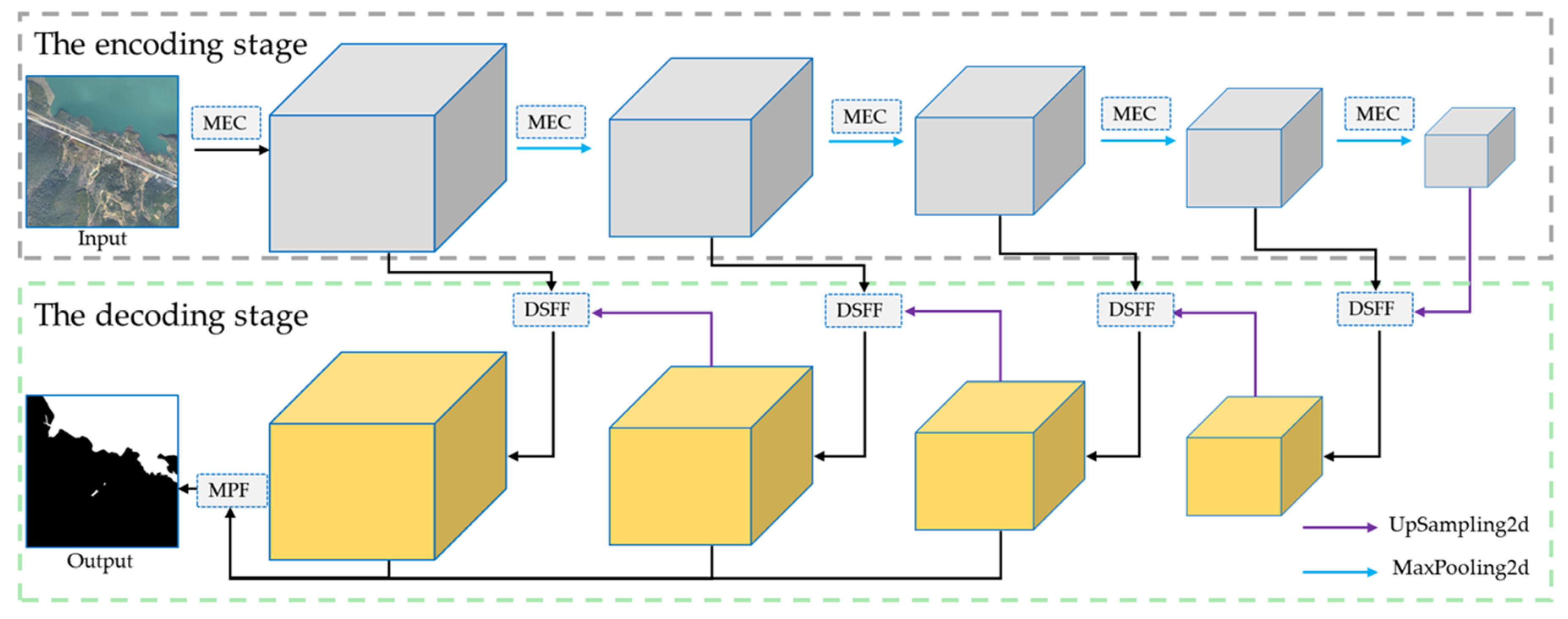
The MECNet mainly consists of three modules. We firstly design a multi-feature extraction and combination module to obtain richer and more diverse features in the encoding stage. The proposed MEC module consists of three different feature extraction sub-modules to model the spatial and channel relationships between feature maps. These sub-modules are (1) a local feature extraction sub-module, (2) a larger receptive-field feature extraction sub-module, and (3) a between-channel feature extraction sub-module. To solve the semantic inconsistency of features from the encoding stage and the decoding stage, an encoder-decoder semantic feature fusion module is established. A simple multi-scale prediction fusion module uses the prediction results from three different scales as input to obtain super fine water-body segmentation contours.
Figure 2 provides an overview of the proposed MECNet, which has an encoder-decoder architecture [9,26,29]. The encoding stage is designed as a bottom-up structure [19]. Four times of max-pooling operations with a stride of two are operated after applying the MEC module for feature extraction. In the decoding stage, the feature maps are sequentially up-sampled up to the size of the original image with a bilinear up-sampling operation with a stride of two. The DSFF module is employed to fuse different features from the encoding and decoding stages at the same scale, whereas the MPF module is used to accurately predict the segmentation map of the water-body.

2.2. Multi-Feature Extraction and Combination Module

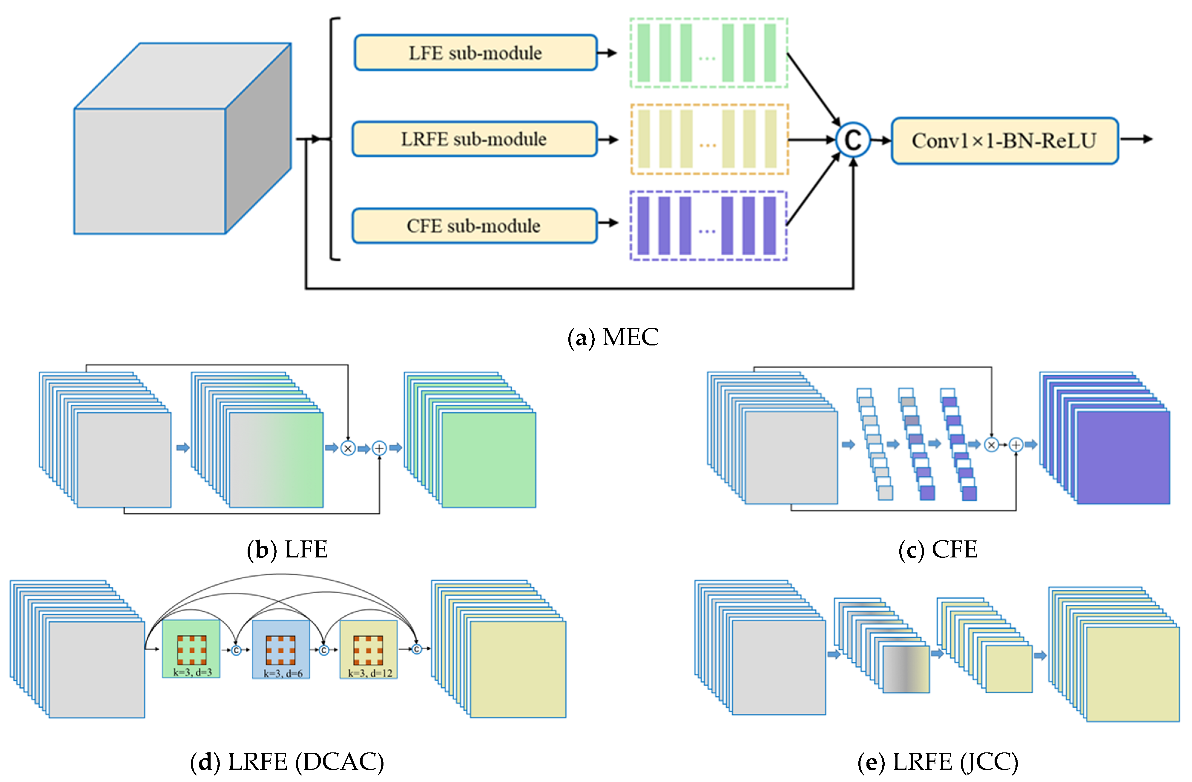
The MEC module is composed of three sub-modules, namely a local feature extraction sub-module (LFE), a longer receptive-field feature extraction sub-module (LRFE) and a feature extraction sub-module for between-channel feature enhancement (CFE). The LFE and LRFE sub-modules are based on the spatial relations of feature maps (i.e., from different receptive-field scenes), and the CFE sub-module is designed to obtain extra rich feature information by modeling the relationships between channels of feature maps.
The LFE sub-module, as shown in Figure 3b, is designed to learn feature maps recording local information. Specifically, we perform a 3×3 convolution with a batch normalization (BN) and a sigmoid function to learn the weight map of local features, and the weight map is multiplied by the input. And then, this result is added to the input as the final output of current layer.
The LRFE sub-module uses a larger receptive field structure. There are two implementation ways: one is to use densely connected atrous convolutions (DCAC), while the other is through pooling operations or convolution with strides. Figure 3d, e shows the structure of these two methods respectively. For an atrous convolutional layer with dilate rate of d and kernel size of K, its receptive field size (RFS) is equal to
R F S 1 = K + ( K 1 ) × ( d 1 )
Stacking convolutional layers can obtain a larger receptive field. For two convolutional layers with receptive field sizes of R1 and R2, the stacked receptive field size is
R F S 2 = R 1 + R 2 1
Using pooling or strides can also obtain a larger receptive field. Since the pooling operation will directly lose local information, we choose convolution with strides. Suppose we have two consecutive convolution layers, the first convolution layer with filter kernel K1 and stride size S1, and the second convolutional layer with filter kernel K2 and stride size S2, the receptive field size is:
R F S 3 = K 1 + ( K 2 1 ) × S 1
In order to choose a more suitable LRFE module, we analyze these two structures in detail. We design three densely connected structures and call them DCAC-large1, DCAC-large2, and DCAC-small. The detailed structures are shown in Table 1. DCAC-large1 and DCAC-large2 have the same receptive field size on each layer, through using fixed kernel size and larger and more dilated rate, and adopting different kernel size and lower dilated rate. And DCAC-small only has a smaller receptive field in the first and second layers than the former two. For the second structure, we design a convolution with kernel size 7 and stride 4, and follows a 3×3 convolution with kernel size 3 and stride 1, and then up-samples to the size of the input. We name this joint structure JCC.
We emphasize the between-channel relationships, and designed a between-Channel Feature Enhancement (CFE) module to learn this relationship (Figure 3c). We firstly use the global pooling operation to get global information of the feature maps, and adopt the full connection to learn the relationship among the values to obtain weights between channels. The weights reflect the relative importance between the channels. Then, they are multiplied with the input channel-wisely and the multiplication result is added to the input.
We design a parallel and a cascade (Figure 4) way to combine the submodules of the MEC. Each feature extraction sub-module in parallel will independently extract features without relying on other intermediate processing results. In the cascade way, the LRFE sub-module further learns the extracted results of LFE sub-module, and the CFE sub-module utilizes the features obtained by the LRFE sub-module, which will acquire features of larger receptive fields step-wise. Notice that the two combinations are identical in terms of the parameters and computational complexity.

2.3. Multi-Scale Prediction Fusion Module

Multi-scale prediction is proved effective in semantic segmentation [10,30,31]. In order to better predict the fine contours of water-bodies, we adopt a simple multi-scale prediction fusion module (MPF, Figure 5). The MPF module optimizes the prediction results of three scales in decoding stage. We first up-sample the third-last and second-last encoder layers to the original image size and concatenate them with the last prediction result. Then, we perform a 1 × 1 convolution with BN and ReLU to increase the number of channels, and respectively use 3 × 3, 5×5, and 7 × 7 convolution with BN and a sigmoid function to learn multi-scale weight information. The weights contain important signals from different receptive fields of the concatenated results, which are multiplied respectively by the weights. Ultimately, we concatenate these results and use a 3 × 3 convolution kernel with BN and 1 × 1 convolution to obtain the final prediction result.

2.4. Encoder-Decoder Semantic Features Fusion Module

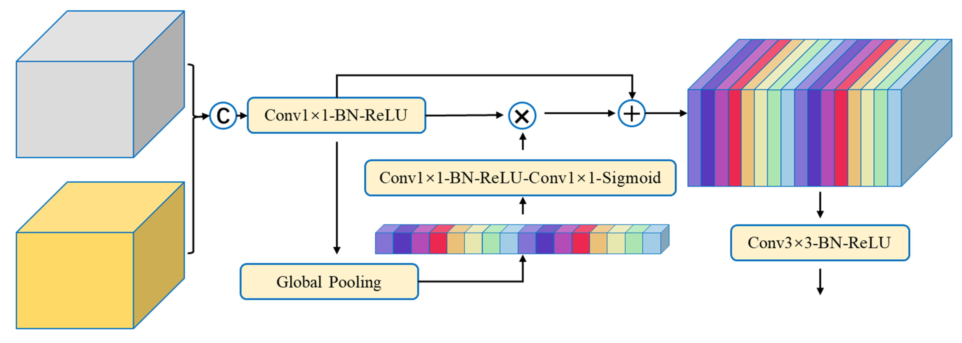
To solve the problem of semantic inconsistency in feature fusion at the decoding stage, we apply the DSFF module (Figure 6), which extends the 3D channel attention module proposed in our previous work [28]. The DSFF is designed for 2D tensors, firstly performs 1 × 1 convolution with BN and ReLU to reduce the channel number of the concatenated feature maps at the same scale from the encoding stage and the decoding stage to half. Then, the global context is generated from the concatenated features by the global pooling and is followed by 1 × 1 convolution with BN and ReLU, and 1 × 1 convolution with a Sigmoid function. It is used as a guide for the fusion of different semantic features, which automatically learns semantic connections between the channels of feature maps. The global context information is multiplied with and added to the concatenated features. Finally, 3 × 3 convolutions with BN and a ReLU are applied to the obtained feature maps. The DSFF module is deployed on different scale features in the decoding stage to achieve efficient fusion of different semantic features.

2.5. The Total Loss Function

The training of deep neural networks become more difficult as the depth of the network increases [20]. In order to train our proposed model more efficiently, we introduce a simple and effective output layer at each scale in the decoding stage and impose loss constraints between its result and ground truth. The output layer consists of a 1 × 1 convolution layer and an up-sampling layer, of which the number of output feature map of the convolution layer is set to 1, and we use bilinear up-sampling. The cross-entropy function L is employed, and the total loss function is as follows:
L t o t a l = α L f i n a l + β i = 1 5 L i
where α and β are the weights for the final prediction results and the sum of the prediction results at each scale in the decoding stage. We set both α and β to 0.5 in our training stage. Following Equation (4), Lfinal denotes the loss between ground truth and the output of the MPF module and L(i) indicates the loss between ground truth and the prediction result of the i-th (i = 1, 2, 3, 4, 5) layer in the decoding stage.

2.6. Implementation Details

We implemented our method using the Pytorch deep learning framework [32]. Considering the limited storage of the GPU, we cropped the original images into patches that measure 512 × 512 pixels with an overlap ratio of 0.5 to eliminate the boundary effects. For a fair comparison between our and other methods, we used the He initialization [33] to initialize our model and other methods in our work and train them without using any pre-trained weights. With the two larger datasets introduced in Section 3.1, we can comprehensively test model learning and generalization abilities. We applied random left-right and top-bottom flipping, Gaussian blur, and HSV transformation to argument the data. We set batch-size to 4 and adopted the Adam (adaptive moment estimation) optimizer [34] and set the learning rate to 1e-4 and the number of epochs to 32 in all experiments.

3. Results and Analysis

3.1. Water-Body Dataset

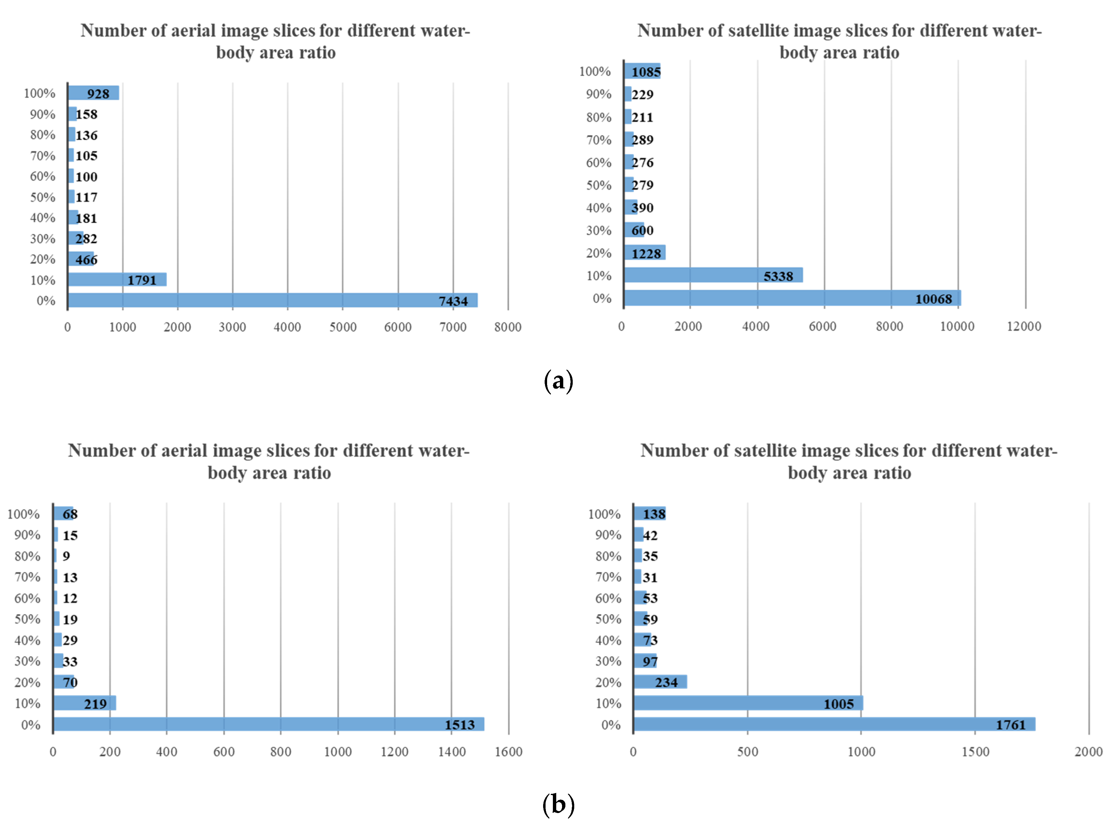
To evaluate our proposed method, we carried out comprehensive experiments in aerial and GF2 (Gaofen2) senses satellite imagery. The aerial images were captured in the Changxing area of Zhejiang Province, China, in 2018. And the dataset has a total of 83 images, from which 63 and 20 are used for training and testing (Figure 1a). The size of each aerial image is 4994 × 4994 pixels, with the ground resolution 0.2 m and three bands (red, green, and blue). From the aerial imagery, it can be observed that there are weeds and silt on both sides of some water-bodies, which makes the delineation of water-bodies more challenging. Moreover, shadows are casted on some water-bodies at the proximity of relatively high ground objects. In addition, there are other types of water-bodies for different applications, such as farmland, fish ponds, etc. The GF2 imagery contains 66 RGB images with a size of 6667 × 6667 pixels and 0.5m ground resolution, of which 48 are used for training and 18 for testing. The images were captured by sensors onboard the GF2 satellite in Jiande, Zhejiang Province, China, in 2018. The edge of the water-bodies is more clearly identifiable from the GF2 satellite images compared to the aerial imagery (Figure 1b). The aerial imagery has been preprocessed with aerial triangulation and ortho-rectification, and the GF2 data has been preprocessed with the quick atmospheric correction (QUAC) method [35] and geometrical rectification. We used the same settings for splitting the training and test sets of the two datasets: 10% of the training set was randomly selected for model validation and cropped to a size of 512 × 512 without overlap. Then, the training set was cropped to the same size with an overlap rate of 0.5. The test set was cropped to 512 × 512 without overlap. We measured a number of different water-body area ratios per tile in the two datasets. The distribution maps of the training and test sets for the number of different area ratio of water-bodies are shown in Figure 7a,b.

3.2. Evaluation Metrics

To compare results quantitatively, we used three evaluation indexes: Precision, Recall, and intersection on union (IoU). They are defined as:
P r e c i s i o n = T P T P + F P
R e c a l l = T P T P + F N
I o U = T P T P + F P + F N
where TP, FP, and FN are the number of true positives, false positives and false negatives, respectively. The precision index describes the accuracy of the prediction of the model and the recall index reflects the recall rate of the water-body, while the IoU is the ratio between the intersection of the pixels of water-bodies detected by the algorithm and the positive pixels and the result of their union. We chose IoU as the main evaluation index.

3.3. Water-Body Segmentation Results

We compared the application of our MECNet on aerial and satellite imagery with five classic and recent methods for general semantic segmentation, which were U-Net [9], RefineNet [10], DeeplabV3+ [26], DANet [36], and CascadePSP [25]. Model performance was compared between their accuracy metrics and through visual interpretation.

3.3.1. The Aerial Imagery

Table 2 shows that our method achieves state-of-the-art accuracy. Our MECNet outperformed the second-best method DANet 2.74% in IoU and 4.32% in recall, which indicated that our method had sufficient advantages in detecting water-bodies and could inspect more complex water samples. However, our model obtained 1.02% lower in precision compared to the DANet. The reason might be that our method recognized some non-water pixels on the edge of water-bodies as water-body pixels. Among methods with similar structures, our MECNet far surpassed U-Net and its variant RefineNet with 5.06% and 4.43% in IoU, which further demonstrated the effectiveness of the three modules we proposed. In addition, our method improved by 3.64% in IoU compared with the latest CascadePSP for target contour optimization. Notably, CascadePSP used the prediction results of DeeplabV3+ as input, aiming to optimize the water-body contour extraction.
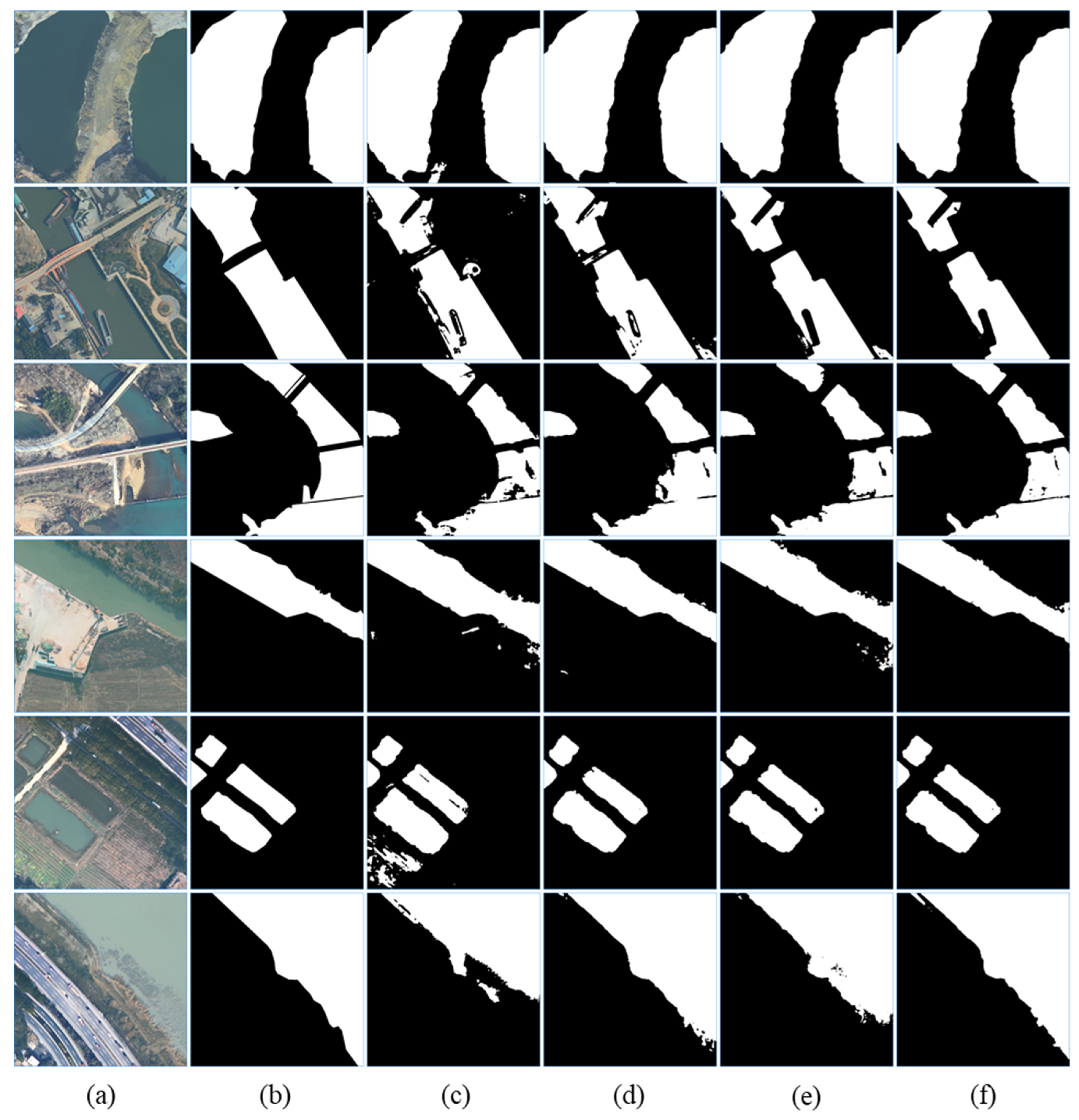
Figure 8 shows the prediction results of different methods. The prediction result produced by our MECNet (Figure 8h) is the closest to the ground-truth (Figure 8b). U-Net (Figure 8c) recognized the shadow as the water-body in the first row and has difficulties in extracting complex edges in the last row as DeeplabV3+ (Figure 8e) and cascadePSP (Figure 8h). In addition, DeeplabV3+, DANet (Figure 8g) and cascadePSP easily identified some non-water bodies as water bodies in the first and second row. RefineNet (Figure 8d) performed poorly in extracting curved water-bodies and moist farmlands, and was commonly interfered by surrounding non-water bodies. For water-body samples with boats in the second row, the other methods are affected, while our method can identify clearer water body boundaries without being confused by the boats.

3.3.2. The Satellite Imagery

The same experiment is applied to the Gaofen2 satellite imagery to further verify the performance of our MECNet. Our proposed method still achieves the best accuracy in IoU (Table 3). Our MECNet surpassed U-Net, RefineNet, DeeplabV3+, DANet and CascadePSP in precision, recall and IoU, except that DANet was slightly better and U-Net was 1.26% higher in terms of recall. Figure 1 shows that the outline of water-bodies in satellite imagery is clearer and simpler than that in aerial imagery, which may be the reason why U-Net, a lightweight and straightforward network structure, could achieve better results than RefineNet and DANet. U-Net was 0.96% and 0.48% higher than the two methods respectively in IoU.
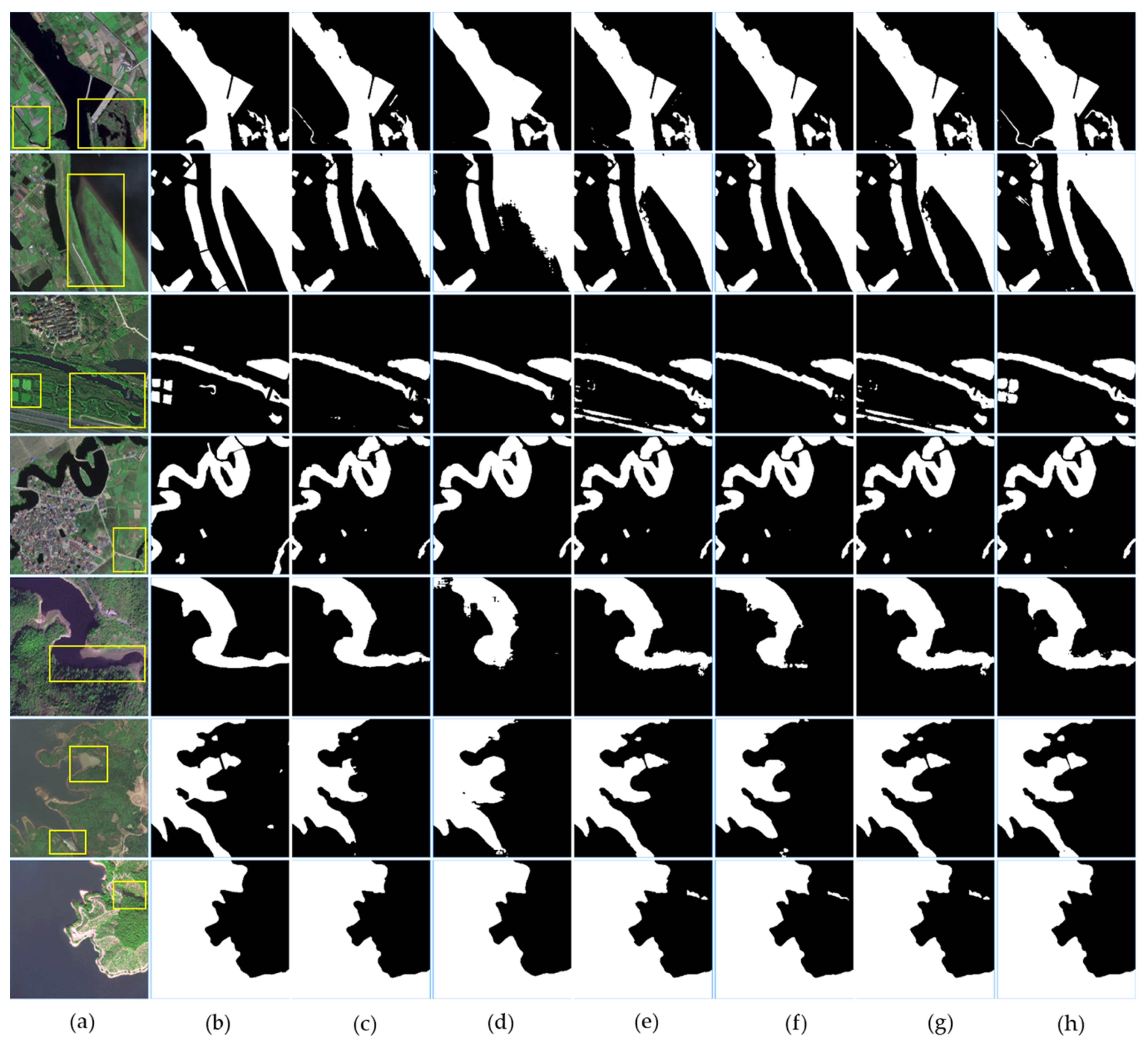
Figure 9 shows the results of some representative water-body segmentations. The water-body contour predicted by our MECNet (Figure 9h) was closest to the ground truth. Some small and special water-body samples, such as small canals and paddy fields in the first and third rows, which were missed out or detected with high errors by other methods, were detected better by our MECNet. Meanwhile, our method clearly identified the complex water-body boundary from the first to third lines. For the meandering water flow, as shown in the fifth row of Figure 9, our method extracted the shadow and inaccurate water-body edges much better compared to the RefineNet and DANet. In a large water area, our method, DeepplabV3+, and CascadePSP could resist the influence of ripples or waves while U-Net, RefineNet, and DANet were affected by them, as shown in the sixth line. However, DeepplabV3+ and CascadePSP easily misrecognized shadows as seen from the last line and was poor at identifying moist farmlands or swamps with small areas in the third row.

3.4. Ablation Studies

In this subsection, we first showed the effect of our proposed MECNet by fully analyzing each part of our method on the performance. Then, we compared the performance of differently designed LRFE sub-modules to find a suitable structure. Finally, we investigated the effectiveness of each and combinations of the sub-modules of the MEC.

3.4.1. MECNet Components

In our proposed MECNet, the MEC module is designed to enhance the feature representation ability at each scale. The MPF module is utilized at the final stage of decoder to fully integrate the results of multi-scale prediction for the fine extraction of water-body contour. And the DSFF is adopted to solve the semantic inconsistency of feature fusion between the encoder and the decoder. In order to verify the performance of our proposed modules, we conducted extensive experiments with different settings (Table 4). We analyzed our methods from quantitative and qualitative perspectives.
Our MECNet achieved significant improvements compared to FCN (Table 4). “FCN + MEC” indicates that the MEC module is only used to replace the convolution layer of the encoding stage in FCN. The “FCN + MEC” improved IoU by 5.31% compared to using FCN alone. From the fourth and fifth lines in Figure 10, it can be observed that the FCN confused some farmland with water-bodies, while an FCN with the MEC module overcomes this challenge. In addition, using the MEC facilitates the identification of edge features from complex water-bodies. These mean the MEC module can obtain more spatial information and enhance the consistency between water and non-water bodies. The MEC with the MPF, which is based on FCN with the MEC module, uses a decoder similar to the U-Net [9] and utilizes the MPF module for multi-scale prediction. Compared with FCN and FCN with the MEC, the design of the MPF module brought 5.75% and 0.44% improvement in IoU respectively, which demonstrated the effectiveness of the MPF. The first and four lines of Figure 10 shows that MEC with the MPF is capable of discriminating shadows. The introduction of the DSFF module further improves the performance of our method. The use of the DSFF module improved the IoU by 0.9% with fewer parameters and FLOPs. It can be seen from the last line of Figure 10 that the DSFF module contributes to a little improvement in the extraction of complex water edges.
To understand the contribution of different modules we proposed in the accurate extraction of the water-bodies, we visualized the feature maps at the last layer of the decoder. We sequentially visualized the feature maps of the backbone FCN, “FCN + MEC”, “MEC + MPF”, and “MEC + MPF + DSFF”, by taking the maximum response to the water body features at each spatial location, as shown in Figure 11.
The backbone FCN has shown to be weak to distinct shadows (Figure 10, first and third rows). It could be observed from Figure 11 that the FCN yielded a greater error response for the shaded features. The introduction of MEC module identified the edges of the water-body better. It also boosted the identification of aquatic plants, silt-obscured water bodies and watered farmland. Introducing the extra MPF leads to a more accurate delineation of water body edges, if we compare (d) and (e) in Figure 11. Finally, an extra feature map fusion technique (DSFF) facilitates a more robust water detection, as can be noticed in the last column of Figure 11.

3.4.2. LRFE Sub-Module

To design and choose a suitable LRFE sub-module, we conducted extensive experiments with FCN as the baseline. Table 5 shows the differences in performance of our designed LRFE sub-modules in VHR aerial imagery. The three methods, i.e., FCN+DCAC-large1, FCN+DCAC-large2 and FCN+DCAC-small (the different structures of LRFE have been listed in Table 1), obtain similar accuracy, but FCN+DCAC-large2 has twice FLOPs compared to others because this model has the largest number of parameters. FCN with DCAC-small has a smaller receptive field than the others, but its accuracy is almost the same as that of the other two DCAC models, which reveals that remote features has less effects on the extraction of water information. FCN with JCC is close to the accuracy of the DCAC model in IoU. Although the parameters of its model were relatively large, it has only 55.29 GFLOPs. Considering the limited hardware resources, we use JCC in the LRFE module.

3.4.3. MEC Module

Based on the observation in Section 2.2, we first separately analyzed the performance of LFE, LRFE and CFE. Then we considered the effects of the two-by-two combinations of these three modules. Finally, we studied the performance of their combination and the impact of different combination ways.
As shown in Table 6, we first implemented FCN using the LFE sub-module, and the IoU increased from 83.99% to 84.78%. The IoU of FCN with the LRFE was 4.17% higher than the baseline. This illustrates that learning features from larger receptive field scenes is more advantageous than learning from local receptive fields, which may be a more important component of spatial feature extraction. FCN using CFE had an increase of 4.36% in the IOU compared to the baseline, which revealed that more robust features could be obtained by learning the relationships between feature map channels. FCN with the CFE was slightly higher than FCN using LRFE, which implied that learning channel information was more effective than learning spatial information in feature extraction. Furthermore, we examined the performance of the two-by-two combinations of three sub-modules, including the combinations of LFE and LRFE, LFE and CFE, and LRFE and CFE. These three different combinations had similar performance, as shown in Table 6. The combination of LFE and LRFE was slightly better than their respective combination with CFE. The reason may be that both LFE and LRFE are based on spatial relationships, while the combination of LFE and CFE, and the combination of LRFE and CFE are combinations based on different relationships. Finally, we investigated two ways of combination among these three sub-modules (Figure 4). The MEC module used a parallel mode was better than a cascade mode in the performance, corresponding to a 0.2% increase. Therefore, we used MEC modules in a parallel mode.

4. Discussion

The boundary of water-bodies in VHR remote sensing imagery is irregular, unclear and complex involving in various scenes. In view of these difficulties, our proposed MEC module adopts three different feature extraction sub-modules to obtain more comprehensive and richer information based on the spatial and channel correlation of feature maps at each scale, compared with other methods mentioned in this paper. Our method is also applicable to other application scenarios, such as semantic segmentation and object detection.
To obtain both high pixel classification accuracy and accurate location, a simple multi-scale prediction fusion (MPF) module is designed to make full use of the prior knowledge, benefiting from our proposed MEC module which provides rich and advanced water-body features in complex remote sensing imagery. This simple and effective design is much more efficient than designing a complex network independently, such as cascadePSP, and will have more advantages in practical application.
We designed a semantic feature fusion module (DSFF) to improve the semantic consistency between the encoder and decoder. This structure not only proved to be effective in crop classification, but is also effective in water-body segmentation in VHR remote sensing imagery. However, this design pays more attention to the global information of feature maps, ignoring the influence of the spatial relationship between feature maps. This will be a focus in our future works.

5. Conclusions

In this study, we innovate based on the encoding–decoding structure to improve fine water-body contour extraction from VHR remote sensing images, including aerial images and satellite images. Three modules are crucial in our method: (1) an MEC module, for automatically extracting richer and more diverse features in the encoding stage and obtain more advanced semantic information for feature fusion in the decoding stage; (2) an MPF module, which attains the fine contour of the water-bodies; (3) a DSFF module, which solves the problem of semantic inconsistency of feature fusion between the encoding stage and the decoding stage. We carried out experiments on VHR aerial and satellite imagery, respectively, and the experiments show that our method achieves state-of-the-art accuracy as well as the best robustness in challenging scenarios. This novel design module for feature extraction can be applied to other application scenarios, such as semantic segmentation and object detection.

Author Contributions

Conceptualization, methodology, and investigation, Z.Z. and S.J.; software and validation, Z.Z.; writing—original draft preparation, Z.Z., M.L., and S.J.; writing—review and editing, Z.Z., M.L., S.J., H.Y., and C.N.; supervision, S.J. and M.L.; funding acquisition, S.J., H.Y., and C.N. All authors have read and agreed to the published version of the manuscript.

Funding

This work was supported by the National Natural Science Foundation of China under Grant 42030102, and the National Key Research and Development Program of China with Grant No. 2018YFB0505003.

Data Availability Statement

We will release our source code at https://github.com/Alisirs/MECNet.

Conflicts of Interest

The authors declare no conflict of interest.

References

  1. Mantzafleri, N.; Psilovikos, A.; Blanta, A. Water quality monitoring and modeling in Lake Kastoria, using GIS. Assessment and management of pollution sources. Water Resour. Manag. 2009, 23, 3221–3254. [Google Scholar] [CrossRef]
  2. Pawełczyk, A. Assessment of health hazard associated with nitrogen compounds in water. Water Sci. Technol. 2012, 66, 666–672. [Google Scholar] [CrossRef] [PubMed]
  3. Haibo, Y.; Zongmin, W.; Hongling, Z.; Yu, G. Water body extraction methods study based on RS and GIS. Procedia Environ. Sci. 2011, 10, 2619–2624. [Google Scholar] [CrossRef] [Green Version]
  4. Frazier, P.S.; Page, K.J. Water body detection and delineation with Landsat TM data. Photogramm. Eng. Remote Sens. 2000, 66, 1461–1468. [Google Scholar]
  5. Gautam, V.K.; Gaurav, P.K.; Murugan, P.; Annadurai, M. Assessment of surface water Dynamicsin Bangalore using WRI, NDWI, MNDWI, supervised classification and KT transformation. Aquat. Procedia 2015, 4, 739–746. [Google Scholar] [CrossRef]
  6. McFeeters, S.K. The use of the Normalized Difference Water Index (NDWI) in the delineation of open water features. Int. J. Remote Sens. 1996, 17, 1425–1432. [Google Scholar] [CrossRef]
  7. Zhao, X.; Wang, P.; Chen, C.; Jiang, T.; Yu, Z.; Guo, B. Waterbody information extraction from remote-sensing images after disasters based on spectral information and characteristic knowledge. Int. J. Remote Sens. 2017, 38, 1404–1422. [Google Scholar] [CrossRef]
  8. Long, J.; Shelhamer, E.; Darrell, T. Fully Convolutional Networks for Semantic Segmentation. IEEE Trans. Pattern Anal. Mach. Intell. 2015, 39, 640–651. [Google Scholar]
  9. Ronneberger, O.; Fischer, P.; Brox, T. U-net: Convolutional networks for biomedical image segmentation. In Proceedings of the International Conference on Medical Image Computing and Computer-Assisted Intervention, Munich, Germany, 5–9 October 2015; pp. 234–241. [Google Scholar]
  10. Lin, G.; Milan, A.; Shen, C.; Reid, I. Refinenet: Multi-path refinement networks for high-resolution semantic segmentation. In Proceedings of the IEEE Conference on Computer Vision and Pattern Recognition, Honolulu, HI, USA, 22–25 July 2017; pp. 1925–1934. [Google Scholar]
  11. Yu, Z.; Feng, C.; Liu, M.-Y.; Ramalingam, S. Casenet: Deep category-aware semantic edge detection. In Proceedings of the IEEE Conference on Computer Vision and Pattern Recognition, Honolulu, HI, USA, 21–26 July 2017; pp. 5964–5973. [Google Scholar]
  12. Bertasius, G.; Shi, J.; Torresani, L. Deepedge: A multi-scale bifurcated deep network for top-down contour detection. In Proceedings of the IEEE Conference on Computer Vision and Pattern Recognition, Boston, MA, USA, 8–10 June 2015; pp. 4380–4389. [Google Scholar]
  13. Xie, S.; Tu, Z. Holistically-nested edge detection. In Proceedings of the IEEE International Conference on Computer Vision, Santiago, Chile, 13–16 December 2015; pp. 1395–1403. [Google Scholar]
  14. Yu, L.; Wang, Z.; Tian, S.; Ye, F.; Ding, J.; Kong, J. Convolutional neural networks for water body extraction from Landsat imagery. Int. J. Comput. Intell. Appl. 2017, 16, 1750001. [Google Scholar] [CrossRef]
  15. Miao, Z.; Fu, K.; Sun, H.; Sun, X.; Yan, M. Automatic water-body segmentation from high-resolution satellite images via deep networks. IEEE Geosci. Remote Sens. Lett. 2018, 15, 602–606. [Google Scholar] [CrossRef]
  16. Li, L.; Yan, Z.; Shen, Q.; Cheng, G.; Gao, L.; Zhang, B. Water body extraction from very high spatial resolution remote sensing data based on fully convolutional networks. Remote Sens. 2019, 11, 1162. [Google Scholar] [CrossRef] [Green Version]
  17. Duan, L.; Hu, X. Multiscale Refinement Network for Water-Body Segmentation in High-Resolution Satellite Imagery. IEEE Geosci. Remote Sens. Lett. 2019, 17, 686–690. [Google Scholar] [CrossRef]
  18. Guo, H.; He, G.; Jiang, W.; Yin, R.; Yan, L.; Leng, W. A Multi-Scale Water Extraction Convolutional Neural Network (MWEN) Method for GaoFen-1 Remote Sensing Images. ISPRS Int. J. Geo Inf. 2020, 9, 189. [Google Scholar] [CrossRef] [Green Version]
  19. Simonyan, K.; Zisserman, A. Very deep convolutional networks for large-scale image recognition. arXiv 2014, arXiv:1409.1556. [Google Scholar]
  20. He, K.; Zhang, X.; Ren, S.; Sun, J. Deep residual learning for image recognition. In Proceedings of the IEEE Conference on Computer Vision and Pattern Recognition, Las Vegas, NV, USA, 27–30 June 2016; pp. 770–778. [Google Scholar]
  21. Huang, G.; Liu, Z.; Van Der Maaten, L.; Weinberger, K.Q. Densely connected convolutional networks. In Proceedings of the IEEE Conference on Computer Vision and Pattern Recognition, Honolulu, HI, USA, 21–26 July 2017; pp. 4700–4708. [Google Scholar]
  22. Zhang, H.; Wu, C.; Zhang, Z.; Zhu, Y.; Zhang, Z.; Lin, H.; Sun, Y.; He, T.; Mueller, J.; Manmatha, R. Resnest: Split-attention networks. arXiv 2020, arXiv:2004.08955. [Google Scholar]
  23. Qin, X.; Zhang, Z.; Huang, C.; Gao, C.; Dehghan, M.; Jagersand, M. Basnet: Boundary-aware salient object detection. In Proceedings of the IEEE Conference on Computer Vision and Pattern Recognition, Long Beach, CA, USA, 16–20 June 2019; pp. 7479–7489. [Google Scholar]
  24. Yu, C.; Wang, J.; Peng, C.; Gao, C.; Yu, G.; Sang, N. Learning a discriminative feature network for semantic segmentation. In Proceedings of the IEEE Conference on Computer Vision and Pattern Recognition, Salt Lake City, UT, USA, 18–22 June 2018; pp. 1857–1866. [Google Scholar]
  25. Cheng, H.K.; Chung, J.; Tai, Y.-W.; Tang, C.-K. CascadePSP: Toward Class-Agnostic and Very High-Resolution Segmentation via Global and Local Refinement. In Proceedings of the IEEE/CVF Conference on Computer Vision and Pattern Recognition, Virtual Conference, Seattle, WA, USA, 14–19 June 2020; pp. 8890–8899. [Google Scholar]
  26. Chen, L.-C.; Zhu, Y.; Papandreou, G.; Schroff, F.; Adam, H. Encoder-decoder with atrous separable convolution for semantic image segmentation. In Proceedings of the European Conference on Computer Vision (ECCV), Munich, Germany, 8–14 September 2018; pp. 801–818. [Google Scholar]
  27. Liu, J.-J.; Hou, Q.; Cheng, M.-M.; Feng, J.; Jiang, J. A simple pooling-based design for real-time salient object detection. In Proceedings of the IEEE Conference on Computer Vision and Pattern Recognition, Long Beach, CA, USA, 16–20 June 2019; pp. 3917–3926. [Google Scholar]
  28. Ji, S.; Zhang, Z.; Zhang, C.; Wei, S.; Lu, M.; Duan, Y. Learning discriminative spatiotemporal features for precise crop classification from multi-temporal satellite images. Int. J. Remote Sens. 2020, 41, 3162–3174. [Google Scholar] [CrossRef]
  29. Badrinarayanan, V.; Kendall, A.; Cipolla, R. Segnet: A deep convolutional encoder-decoder architecture for image segmentation. IEEE Trans. Pattern Anal. Mach. Intell. 2017, 39, 2481–2495. [Google Scholar] [CrossRef]
  30. Wei, S.; Ji, S.; Lu, M. Toward automatic building footprint delineation from aerial images using cnn and regularization. IEEE Trans. Geosci. Remote Sens. 2019, 58, 2178–2189. [Google Scholar] [CrossRef]
  31. Gu, Y.; Lu, X.; Yang, L.; Zhang, B.; Yu, D.; Zhao, Y.; Gao, L.; Wu, L.; Zhou, T. Automatic lung nodule detection using a 3D deep convolutional neural network combined with a multi-scale prediction strategy in chest CTs. Comput. Biol. Med. 2018, 103, 220–231. [Google Scholar] [CrossRef]
  32. Bernstein, L.S.; Adler-Golden, S.M.; Sundberg, R.L.; Levine, R.Y.; Perkins, T.C.; Berk, A.; Ratkowski, A.J.; Felde, G.; Hoke, M.L. Validation of the QUick Atmospheric Correction (QUAC) algorithm for VNIR-SWIR multi-and hyperspectral imagery. Proc. SPIE 2005, 5806, 668–678. [Google Scholar]
  33. Paszke, A.; Gross, S.; Massa, F.; Lerer, A.; Bradbury, J.; Chanan, G.; Killeen, T.; Lin, Z.; Gimelshein, N.; Antiga, L. Pytorch: An imperative style, high-performance deep learning library. In Proceedings of the Advances in Neural Information Processing Systems, Vancouver, BC, Canada, 8–14 December 2019; pp. 8026–8037. [Google Scholar]
  34. He, K.; Zhang, X.; Ren, S.; Sun, J. Delving deep into rectifiers: Surpassing human-level performance on imagenet classification. In Proceedings of the IEEE International Conference on Computer Vision, Santiago, Chile, 13–16 December 2015; pp. 1026–1034. [Google Scholar]
  35. Kingma, D.P.; Ba, J. Adam: A method for stochastic optimization. arXiv 2014, arXiv:1412.6980. [Google Scholar]
  36. Fu, J.; Liu, J.; Tian, H.; Li, Y.; Bao, Y.; Fang, Z.; Lu, H. Dual attention network for scene segmentation. In Proceedings of the IEEE Conference on Computer Vision and Pattern Recognition, Long Beach, CA, USA, 16–20 June 2019; pp. 3146–3154. [Google Scholar]
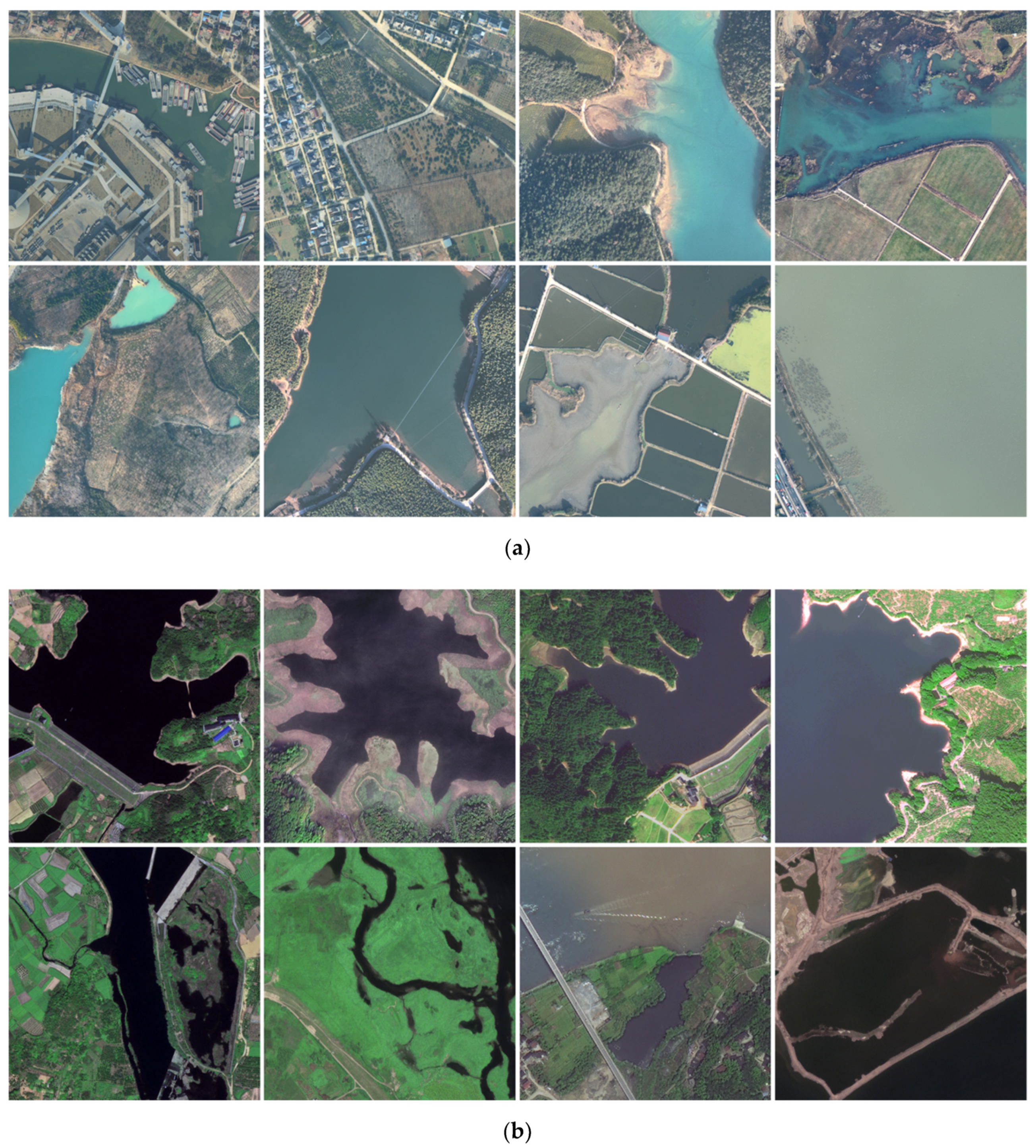
Figure 1. Some typical water-body samples (a) in VHR aerial images and (b) Gaofen2 (GF2) satellite images
Remotesensing 13 01912 g001
Figure 2. An overview of our proposed Multi-feature Extraction and Combination Network (MECNet). MECNet has three modules: Multi-feature Extraction and Combination (MEC), encoder and Decoder Semantic Feature Fusion (DSFF), and Multi-scale Prediction Fusion (MPF).
Remotesensing 13 01912 g002
Figure 3. The details of multi-feature extraction and combination module. (a) The MEC (Multi-feature Extraction and Combination) module consists of (b) a Local Feature Extraction (LFE) sub-module, (c) a between-channel feature enhancement module (CFE) and a longer receptive-field feature extraction sub-module (LRFE): (d) DCAC (Densely Connected Atrous Convolutions, and (e) JCC (Joint Conv7-S4-Conv3-S1, for the longer receptive field feature extraction.
Remotesensing 13 01912 g003
Figure 4. Two ways to combine different feature sub-modules in the MEC (Multi-feature Extraction and Combination), Left: in a parallel way. Right: in a cascade way.
Remotesensing 13 01912 g004
Figure 5. MPF: Multi-scale Prediction Fusion module.
Remotesensing 13 01912 g005
Figure 6. Different Semantic Feature Fusion module, DSFF.
Remotesensing 13 01912 g006
Figure 7. Distributions of the number of image slices over water-body area ratios, for (a) the two training sets and (b) test sets. The horizontal axis denotes number of image tiles. The vertical axis indicates the area ratio of water bodies in a single remote sensing image tile, e.g., 0% means that there is no water-body in an image slice, and 10% means that the area ratio of water bodies on an image belongs to (0%, 10%).
Remotesensing 13 01912 g007
Figure 8. Qualitative comparisons with other empirical networks on the aerial imagery. (a) Images. (b) Ground-truth. (c) U-Net. (d) RefineNet. (e) DeeplabV3+. (f) DANet. (g) CascadePSP. (h) MECNet (ours).
Remotesensing 13 01912 g008
Figure 9. Water-body Segmentation results of several methods on the VHR satellite imagery. (a) Images. (b) Ground-truth. (c) U-Net. (d) RefineNet. (e) DeeplabV3+. (f) DANet. (g) CascadePSP. (h) MECNet (ours). The yellow rectangle represents several complex areas with water-bodies, such as ditches and paddy fields in the first and third rows, rivers with severe ripples in the penultimate row, etc.
Remotesensing 13 01912 g009
Figure 10. Example results of our proposed MECNet on the VHR aerial imagery. (a) Images. (b) Ground-truth. (c) FCN-8s. (d) FCN + MEC. (e) MEC + MPF. (f) MEC + MPF + DSFF (MECNet).
Remotesensing 13 01912 g010
Figure 11. Visualization of feature maps located at the last layer of the decoder of different network structures. (a) Images. (b) Ground-truth. (c) FCN-8s. (d) FCN + MEC. (e) MEC + MPF. (f) MEC + MPF + DSFF (MECNet).
Remotesensing 13 01912 g011
Table 1. The various longer receptive-field feature extraction (LRFE) sub-modules designed in this study. Layeri represents the i-th layer of the encoder (i belongs to (1, 2, 3, 4, 5)), RFS indicates the receptive field size relative to the input.
DCAC-Large1DCAC-Large2
LayeriKernel SizeDilated RateRFSKernel SizeDilated RateRFS
layer13(3, 6, 12, 18, 24)1317(3, 6, 12)129
layer23(3, 6, 12, 18)825(3, 6, 12)87
layer33(3, 6, 12)453(3, 6, 12)45
layer43(1, 3, 6)233(1, 3, 6)23
layer53(1, 2, 3)153(1, 2, 3)15
DCAC-SmallJCC
layeriKernel SizeDilated RateRFSKernel SizeDilated RateRFS
layer13(3, 6, 12)457, 3(1)15
layer23(3, 6, 12)457, 3(1)15
layer33(3, 6, 12)457, 3(1)15
layer43(1, 3, 6)237, 3(1)15
layer53(1, 2, 3)157, 3(1)15
Table 2. The accuracy metrics of ours and other empirical networks using aerial imagery. The bold format indicates the best results for each network in each evaluation metric.
MethodBackbonePrecisionRecallIOU
U-Net-0.9076 0.9374 0.8558
RefineNetresnet1010.8741 0.9844 0.8621
DeeplabV3+resnet1010.9140 0.9417 0.8650
DANetresnet1010.92590.9456 0.8790
CascadePSPDeeplabV3+&resnet500.9203 0.9409 0.8700
MECNet (ours)-0.9157 0.98880.9064
Table 3. Numerical comparisons with other empirical networks on the VHR satellite imagery. The bold format indicates the best results for each network in each evaluation metric.
MethodBackbonePrecisionRecallIOU
U-Net-0.9119 0.9756 0.8916
RefineNetresnet1010.9176 0.9578 0.8820
DeeplabV3+resnet1010.9379 0.9582 0.9010
DANetresnet1010.9156 0.9658 0.8868
CascadePSPDeeplabV3+&resnet500.9378 0.9586 0.9013
MECNet (ours)-0.94080.96300.9080
Table 4. Our MECNet improve the performance of water-body segmentation on the VHR aerial imagery dataset. Parameters and FLOPs mean the parameters and floating-point operations per method. ‘M’: million, ‘B’: Billion.
MethodParameter (M)Flops (B)IoU
FCN-8s15.31 81.00 0.8399
FCN + MEC26.11 105.59 0.8930
MEC + MPF35.46 254.29 0.8974
MEC + MPF + DSFF (MECNet)30.07 185.58 0.9064
Table 5. The performance of differently designed LRFE sub-modules in VHR aerial imagery.
MethodParameters (M)FLOPs(G)IoU
FCN15.31 81.10 0.8399
FCN+DCAC-large112.88 140.96 0.8801
FCN+DCAC-large213.39 248.30 0.8841
FCN+DCAC-small12.70 106.57 0.8823
FCN+JCC19.08 55.29 0.8816
Table 6. Detailed performance of MEC module with different settings. ‘(C)’ means the MEC module adopts a cascade way for the three sub-modules. ‘(P)’ means the MEC module uses a parallel way for the three sub-modules.
MethodLFELRFECFEIoU
FCN 0.8399
FCN 0.8478
FCN 0.8816
FCN 0.8835
FCN 0.8857
FCN 0.8851
FCN 0.8855
FCN (C)0.8910
FCN (P)0.8930
Publisher’s Note: MDPI stays neutral with regard to jurisdictional claims in published maps and institutional affiliations.