Retrieval of Secchi Disk Depth in Turbid Lakes from GOCI Based on a New Semi-Analytical Algorithm

Abstract

The accurate remote estimation of the Secchi disk depth (Z_SD) in turbid waters is essential in the monitoring the ecological environment of lakes. Using the field measured Z_SD and the remote sensing reflectance (Rrs(λ)) data, a new semi-analytical algorithm (denoted as Z_SDZ) for retrieving Z_SD was developed from Rrs(λ), and it was applied to Geostationary Ocean Color Imager (GOCI) images in extremely turbid waters. Our results are as follows: (1) the Z_SDZ performs well in estimating Z_SD in turbid water bodies (0.15 m < Z_SD < 2.5 m). By validating with the field measured data that were collected in four turbid inland lakes, the determination coefficient (R²) is determined to be 0.89, with a mean absolute square percentage error (MAPE) of 22.39%, and root mean square error (RMSE) of 0.24 m. (2) The Z_SDZ improved the retrieval accuracy of Z_SD in turbid waters and outperformed the existing semi-analytical schemes. (3) The developed algorithm and GOCI data are in order to map the hourly variation of Z_SD in turbid inland waters, the GOCI-derived results reveal a significant spatiotemporal variation in our study region, which are significantly driven by wind forcing. This study can provide a new approach for estimating water transparency in turbid waters, offering important support for the management of inland waters.

1. Introduction

Water transparency, which has been widely and regularly measured with Secchi disk in both limnology and oceanography, is key information for assessing the water quality and trophic state. Secchi disk depth (Z_SD, m) is the depth at which the disk, lowered from the surface, is no longer visible to the observer, and is a measure of transparency or vertical visibility in the water body. The values of Z_SD depend on the intensity of light, water molecules, and optical components (e.g., chlorophyll-a and suspended matter), and they play a key role in understanding aquatic environment variations and biogeochemical processes [1]. Traditional methods of estimating Z_SD largely depend on cruise surveys, which are laborious and time-consuming. The large coverage characteristics of satellite data makes it a perfect tool for describing the spatial and temporal variability of Z_SD [2].

Substantial efforts, which are based on remote sensing methods, have been made to obtain Z_SD for describing the spatiotemporal variability of water properties in marine, coastal, and inland waters [3,4,5,6,7]. They can be mainly divided into two strategies: empirical and semi-analytical approaches. (1) empirical methods: Binding et al. [8] used remote-sensing reflectance at 550 nm to estimate Z_SD in Great Lakes based on multi-source satellite data. Shi et al. [5] also estimated Z_SD in Lake Taihu by constructing a linear regression model between Z_SD and MODIS-Aqua reflectance at 645 nm. However, the empirical methods have the characteristic of location-dependency and may not be portable to other waters. (2) semi-analytical methods: Preisendorfer et al. proposed a semi-analytical approach for estimating inherent optical properties (IOPs) [9] based on classical underwater visibility theory; this approach has been applied to estimate Z_SD [7]; however, the results from this approach did not agree well with field observations and human experiences, and a new semi-analytical model (denoted as Z_SDV6) based on the radiative transfer theory was proposed by Lee et al. [10] to retrieve Z_SD. Shang et al. subsequently verified the encouraging performance of the new method [11].

This new model was developed and validated with a large data covering different IOPs conditions, including marine, coastal, and inland waters (Z_SD range of 0.1–30 m), and received excellent results (~18% average absolute difference, R² = 0.96) [12]. By this method, the inherent optical properties (IOPs) were first estimated while using the quasi-analytical algorithm (QAA), and then positing the reference wavelength at 550 or 670 nm further derived the Z_SD. However, several obvious limitations of the original QAA become evident for applications in inland turbid waters [6,13,14,15,16]. Firstly, the estimation method of the total absorption coefficient at the reference wavelength (550 or 670 nm) does not work in inland turbid waters with lower absorption, but high scattering coefficients; secondly, the original coefficients of the IOPs were calibrated while using the data from marine and coastal waters and inland waters. The Z_SD in turbid water is much lower than in oceanic water or coastal waters, and so the Z_SD model must be reevaluated for these turbid conditions. Moreover, vertical heterogeneous distribution of water constituents and complex optical properties in turbid lakes challenge the validation of parameters in the semi-analytical model of Z_SD that was proposed by Lee et al. [10]. Therefore, an improved semi-analytical algorithm is needed to retrieve Z_SD in turbid waters.

The Geostationary Ocean Color Imager (GOCI), an ocean color satellite imager that has been set in geostationary orbit, provides eight images during the daytime from 8:30 to 16:30 local time. With its eight bands from visible to near-infrared spectral region (412~865 nm) and one hourly short temporal resolutions, GOCI has been confirmed as an ideal satellite sensor with high signal-to-noise ratios (SNR) for mapping suspended particulate matter, colored dissolved organic matter (CDOM), and harmful algal blooms [13,17,18,19]. Although the application of GOCI data for Z_SD estimation has seldom been reported in inland turbid waters, it could be of great significance for the observation of Z_SD in inland turbid lakes.

The Z_SD of Lake Taihu and Lake Hongze were estimated based on in-situ data and GOCI images to improve the algorithm of retrieving Z_SD in inland turbid water. The main objectives of this study were: (1) to develop a new semi-analytical algorithm of Z_SD for inland turbid waters, (2) compare the performance of the new scheme with the existing semi-analytical algorithm, and (3) to obtain the spatiotemporal dynamic characteristics of Z_SD from GOCI observations.

2. Materials and Methods

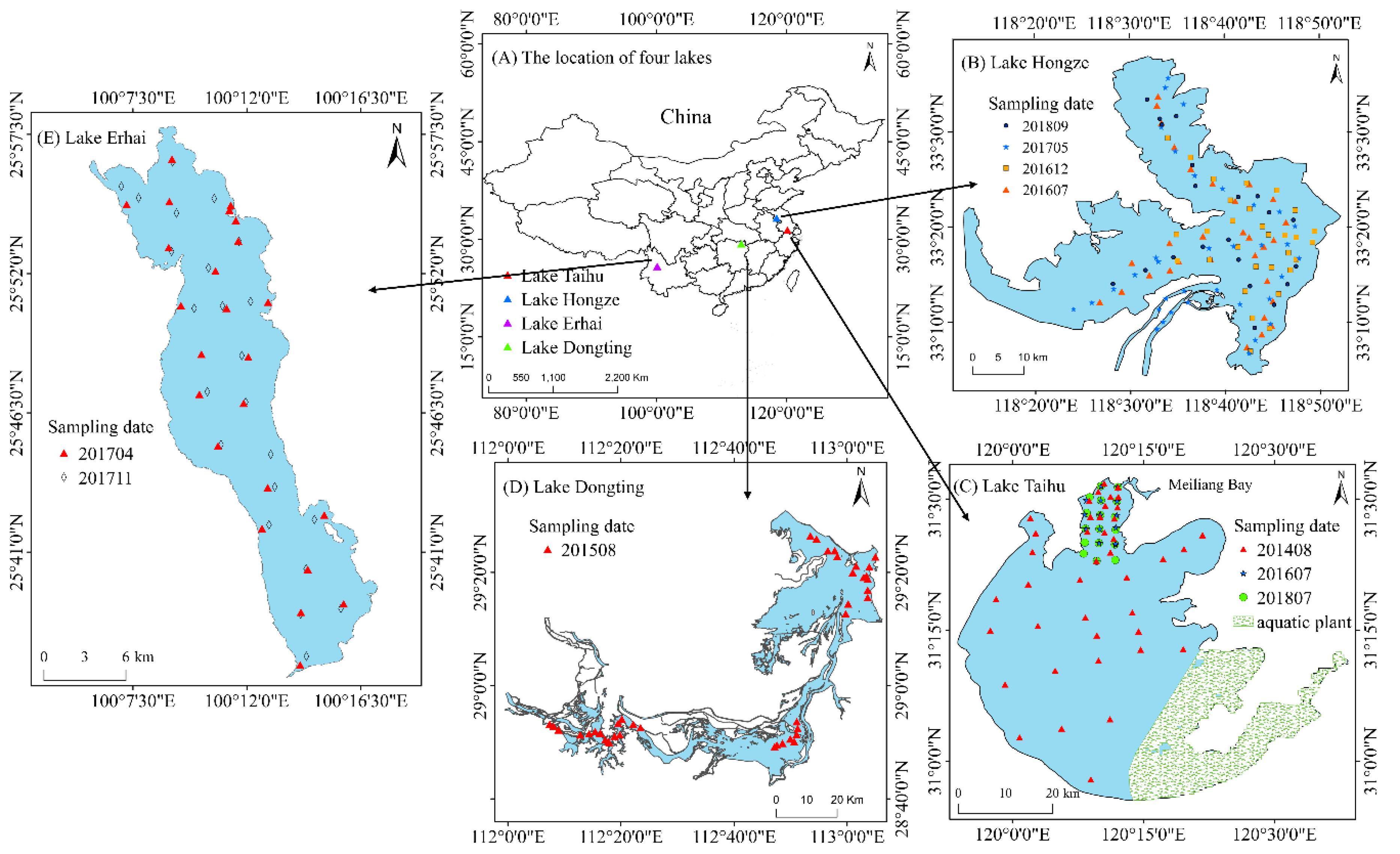
2.1. Study Area

Four turbid waters—Lake Dongting (28°30′–30°20′N, 111°40′–113°10′E), Lake Taihu (30°55′–31°32′N, 118°52′–120°36′E), Lake Hongze (33°06′–33°40′N, 118°10′–118°52′E), and Lake Erhai (25°61′–25°98′N, 100°08′–100°31′E)—are observed in our study. As the second, third, and fourth largest freshwater lakes in China, Lake Dongting, Lake Taihu, and Lake Hongze have water areas of ~2794 km², ~2338 km², and ~1577 km², respectively (Figure 1). Lake Erhai is the second largest freshwater lake in Yunnan Province. Lake Dongting has a mean water depth of 1.9 m and a maximum depth of ~5.5 m. Lake Taihu has a mean water depth of 1.9 m and a maximum depth of ~2.6 m. Lake Hongze has a mean water depth of 1.8 m and a maximum depth of ~4.5 m. Lake Erhai has a mean water depth of 10 m and maximum depth of ~20 m. Over the past few decades, because of environmental overload from catchments, the aquatic ecosystems of lakes have faced water quality deterioration and reduced biodiversity. Blue-green algae outbreaks in these lakes seriously affect aquatic biodiversity, tourism, and the health of nearby residents. Lake Taihu is characterized by hypereutrophic and high turbidity due to high levels of primary production and high concentrations of suspended sediments; Lake Hongze is characterized by mesotrophic and high turbidity due to a large amount of sediment and terrestrial debris being carried from the Huai River and human activities [20]. Similar to the above two lakes, Lake Dongting has also experienced eutrophication in recent years due to anthropogenic activities and environmental change [21].

2.2. In-Situ Water Quality Data and Spectra Data Collection

From 2014 to 2018, the remote-sensing reflectance ($R_{rs}\left(\lambda \right)$) and the underwater downward irradiance ($E_d\left(\lambda ,z\right)$) were measured in-situ by taking 232 samples (87 samples in Lake Hongze, 58 in Lake Taihu, 40 in Lake Dongting, and 47 in Lake Erhai) in ten cruise campaigns (Figure 1). The $R_{rs}\left(\lambda \right)$ data were field-measured while using an Analytical Spectral Devices (ASD) Inc. FieldSpec Pro. Full details of the measurement process of $R_{rs}\left(\lambda \right)$ are provided by previous studies [22,23]. At each sampling site, the total radiance ($L_t$), the sky-viewing radiance ($L_{sky}$), and the radiance reflected by a standard gray panel ($L_p$) were collected. The $R_{rs}\left(\lambda \right)$ can be computed with the following equation:

$$R_{rs}\left(\lambda \right)={\rho }_{\mathrm{p}}\left(L_t-r_{aw}{L}_{sky}\right)/\left(\pi L_p\right)$$

(1)

where the ${\rho }_{\mathrm{p}}$ is the reflectance of the grey panel.

The diffuse attenuation coefficient $K_d\left(\lambda \right)$ was field collected while using an underwater spectroradiometer (TriOS Mess- und Datentechnik GmbH, Rastede, Germany). With a spectral channels range of 320 to 950 nm, the spectral sampling interval of spectroradiometer is 3.3 nm, which was subsequently interpolated to a new resolution of 1 nm in indoor data processing. The spectra of underwater downward irradiance $E_d\left(\lambda ,z\right)$ at different sampling depths ($z$ = 0.2, 0.4,…….,1.2 m) were measured by the spectroradiometer [21]. $K_d\left(\lambda \right)$ was calculated by applying a non-linear fit between $E_d\left(\lambda ,0^{-}\right)$ and depth $\left(z\right)$:

$$E_d\left(\lambda ,0^{-}\right)=E_d\left(\lambda ,0^{-}\right)\ast \exp \left(-K_d\left(\lambda \right)\ast z\right)$$

(2)

$K_d\left(\lambda \right)$ was only determined if R² of non-linear fit regressions was greater than 0.95 and the number of depths must be no less than 3 [24].

Secchi disk depth (Z_SD) measurements and water samples were simultaneously collected at each sampling site. The Secchi disk is lowered into a body of water by an observer until it disappears from view; the depth at which it is no longer visible is recorded as the Z_SD value. One skilled person carried out all of the measurements in order to decrease artificial error. At the same time, in situ water samples were collected using Niskin bottles at a depth of 50 cm under the surface and were kept in containers at −20 °C for laboratory analysis. Whthin the next five days, the water samples were filtered and measured in the laboratory. The measured parameters of water samples in laboratory analysis included chlorophyll-a (Chla), total suspended matter (TSM), and organic/ inorganic suspended matter (OSM/ISM) concentrations, which were determined using the method that was described by Chen et al. [25]. Note that Lake Erhai has not field measured $K_d\left(\lambda \right)$ data used in this study. Finally, the total datasets of 232 samples were divided into two groups, one of which consisted of 137 samples, approximately 58% of the total number of samples, was used to calibrate the model; the remaining group was used to validate the accuracy of the model.

2.3. Satellite Data and Preprocessing

GOCI images, which were captured in Lake Hongze and Lake Taihu from 2014 to 2018, were downloaded from the Korea Ocean Satellite Center (KOSC). The 6S method (Second Simulation of the Satellite Signal in the Solar Spectrum, 6S) was used to correct the GOCI Level-1B data, which are the same as the latest research [19,22]. After image data pre-processing, these data were used to validate the performance of 6s model and estimate the Z_SD in Lake Hongze and Lake Taihu. During the cruise campaigns that were conducted from 2014 to 2018, the measurement time of a total of 125 points (69 points in Lake Hongze and 56 in Lake Taihu) was close to GOCI imaging time (± 1 h). These sampling points were selected for further validation of the accuracy of 6S atmospheric correction.

2.4. Wind Speed Data Collection

Hourly wind data from 2015–2018 in Dongshan meteorological station (31°4′N, 120°26′E) near Lake Taiyhu and Xuyi meteorological station (33°42′N, 118°32′E) near Lake Hongze were obtained from the China Meteorological Data Sharing Service System (http://cdc.c,a.gov.cn/home.do). These data were recorded per 1 h, which could be matched with the GOCI imaging time.

2.5. Data analyses and Accuracy Assessment

Correlation analyses were performed with OriginPro 2018 software. Three evaluation indicators, including the coefficient of determination (R²), the mean absolute square percentage error (MAPE), and root mean square error (RMSE), were selected to characterize the performance of the model:

$$\mathrm{MAPE}=\frac{1}{n}{{\displaystyle \sum }}_{i=1}^n\left(\left|v_{meas}^i-v_{pred}^i\right|/v_{meas}^i\right)\ast 100\%$$

(3)

$$\mathrm{MAPE}=\frac{\sqrt{{{\displaystyle \sum }}_{i=1}^n\left(v_{meas}^i-v_{pred}^i\right)}}{n}$$

(4)

where the $v_{pred}^i$ and $v_{meas}^i$ are the estimated and measured values, respectively; n is the number of samples.

2.6. Z_SDZ Algorithm

A new semi-analytical algorithm (denoted as Z_SDZ) that is suitable for estimating Z_SD in inland turbid waters was developed based on the original Z_SDV6 by Lee et al. [10] and modified based on the in-situ data.

Table 1. Steps of Z_SDZ algorithm (a new semi-analytical algorithm).

Step	Property	Expression	Approach
1	$r_{rs}\left(\lambda \right)$	$r_{rs}\left(\lambda \right)=\frac{R_{rs}\left(\lambda \right)}{0.52+1.7R_{rs}\left(\lambda \right)}$	Semi-analytical
2	$u\left(\lambda \right)$	$u\left(\lambda \right)=\frac{-\mathrm{g}0+\sqrt{{\left(\mathrm{g}0\right)}^2+4\mathrm{g}1\ast r_{rs}\left(\lambda \right)}}{2{\mathrm{g}}_1}$ $\mathrm{g}0=0.084, \mathrm{g}1=0.17$	Semi-analytical
3	$a\left(745\right)$	$a\left({\lambda }_0\right)=a_{\mathrm{w}}\left({\lambda }_0\right)+△a\left({\lambda }_0\right)\approx a_{\mathrm{w}}\left({\lambda }_0\right)$ ${\lambda }_0=745$	Empirical
4	$b_b\left(745\right)$	$b_b\left({\lambda }_0\right)=\frac{u\left({\lambda }_0\right)a\left({\lambda }_0\right)}{1-u\left({\lambda }_0\right)}$, ${\lambda }_0=745$	Analytical
5	$K_d\left({\lambda }_0\right)$	$K_d\left({\lambda }_0\right)=\left(1+{\mathrm{m}}_0{\ast \mathsf{\theta }}_{\mathrm{s}}\right)a\left({\lambda }_0\right)+$ ${\mathrm{m}}_1\left(1-{\mathrm{m}}_2\exp \left(-{\mathrm{m}}_{3}a\left({\lambda }_0\right)\right)\right)b_b\left({\lambda }_0\right)$ ${\mathrm{m}}_0=0.0124,{\mathrm{m}}_1=3.16,{\mathrm{m}}_2=0.52,{\mathrm{m}}_3=10.8$	Semi-analytical
6	$K_d\left(555\right)$	$K_d\left(555\right)=b\ast K_d\left(745\right)+c$ $b=0.99, c=-1.96$	Empirical
7	${\mathrm{Z}}_{\mathrm{SD}}$	$Z_{SD}=\frac{1}{2.5\mathrm{Min}\left(K_d^{tr}\right)}\ln (\frac{\left|0.14-R_{rs}^{tr}\right|}{0.013})$ $\mathrm{Min}\left(K_d^{tr}\right)=K_d\left(555\right), R_{rs}^{tr}=R_{rs}\left(555\right)$	Semi-analytical

lists the derivation flowchart of Z_SDZ algorithm and the corresponding expressions. Two parts (part I and part II) are contained in the new algorithm.

2.6.1. Part I

In step 1, $r_{rs}\left(\lambda \right)$ can be calculated as [26]:

$$r_{rs}\left(\lambda \right)=\frac{R_{rs}\left(\lambda \right)}{0.52+1.7R_{rs}\left(\lambda \right)}$$

(5)

In step 2, $u\left(\lambda \right)$ can be calculated as [26]:

$$u\left(\lambda \right)=\frac{-\mathrm{g}0+\sqrt{{\left(\mathrm{g}0\right)}^2+4\mathrm{g}1\ast r_{rs}\left(\lambda \right)}}{2{\mathrm{g}}_1}$$

(6)

where g0 =0.084 and g1 = 0.17 in Z_SDZ algorithm, which were suggested for high scattering waters by [15].

In step 3, $a\left({\lambda }_0\right)$. can be obtained based on the assumption that the $a_{\mathrm{w}}\left({\lambda }_0\right)$ is dominant at ${\lambda }_0$.

$$a\left({\lambda }_0\right)=a_{\mathrm{w}}\left({\lambda }_0\right)+△a\left({\lambda }_0\right)\approx a_{\mathrm{w}}\left({\lambda }_0\right)$$

(7)

In original Z_SDV6 algorithm that was proposed by Lee et al. [10], $a\left({\lambda }_0\right)$ is the absorption of dissolved components and detritus at original reference wavelength (550 nm or 670 nm). However, poor accuracy can be obtained by deriving $△a\left(550\right)$ or $△a\left(670\right)$, and further leading to poorer performance of $a\left({\lambda }_0\right)$ in turbid waterbodies. Moreover, an ambiguous extrapolation index of the aerosol model usually leads to the poor estimation of $R_{rs}$ from satellite images at short wavelengths in highly turbid inland waters [27]. These defects will propagate to the next steps and affect the accuracy of the model. One way to overcome this shortcoming is to first shift the reference wavelength to longer bands [6,28]. There are two longer NIR (745 nm and 845 nm) that meet the above conditions given the band setting of the GOCI image. However, poor performance of atmospheric correction existed at 865nm. Therefore, in the modified algorithm of Z_SDZ, the reference wavelength of $a\left({\lambda }_0\right)$ will be shifted to 745 nm, and the $a\left({\lambda }_0\right)$ is considered to be equal to the absorption coefficient of pure water at 745 nm, $a_{\mathrm{w}}\left(745\right)$. Samplings of 745 nm of GOCI are determined in this step, other sensors with longer NIR band, such as the 740 nm of Sentinel-2, can also be selected as reference wavelength when applying the Z_SDZ to other study areas.

In step 4, $b_b\left({\lambda }_0\right)$ can be calculated as:

$$b_b\left({\lambda }_0\right)=\frac{u\left({\lambda }_0\right)a\left({\lambda }_0\right)}{1-u\left({\lambda }_0\right)}$$

(8)

In the step 5, $K_d\left({\lambda }_0\right)$ can be calculated as:

$$K_d\left({\lambda }_0\right)=\left(1+{\mathrm{m}}_0{\ast \mathsf{\theta }}_{\mathrm{s}}\right)a\left({\lambda }_0\right)+{\mathrm{m}}_1\left(1-{\mathrm{m}}_2\exp \left(-{\mathrm{m}}_{3}a\left({\lambda }_0\right)\right)\right)b_b\left({\lambda }_0\right)$$

(9)

In Z_SDV6 algorithm, the original values of parameters (m0~3) were determined while using Hydrolight simulations on oligotrophic waters and Case-1 model of Morel et al. [29] for optical properties, where the input inherent optical properties (IOPs) were kept vertically constant [30]. Therefore, parameters (m0~3) should be retuned for turbid waters. Parameters (m0~3) were retuned using our calibration data (137 samples) in order to meet the application of turbid waters, similar to Lee et al. [30]. In detail, we fixed the same values for m1, m2, and m3, but varied m0, and the optimal value of m0 was further confirmed based on nonlinear best fit. The values of m1~m3 were obtained in the same way. The final values of the four model parameters (m0~3) were 0.0124, 3.16, 0.52, and 10.8, respectively. After retuning, Figure 2A presents the match up points between the field measured and the retrieved $K_d\left(745\right)$. All of the points were closely distributed along the 1:1 line with low MAPE (10.24%) and RMSE (0.81 m⁻¹), which suggests that the retuned values of parameters (m0~3) are acceptable for estimation of $K_d\left(745\right)$.

In step 6, $K_d\left(\lambda \right)$ can be calculated based on line regression between $K_d\left(\lambda \right)$ and $K_d\left({\lambda }_0\right)$, as:

$$K_d\left(\lambda \right)=b\ast K_d\left({\lambda }_0\right)+c$$

(10)

where b and c are the coefficient and intercept of the line regression equation, respectively, which can be determined by the field measured data.

2.5.2. Part II

In part II, the Z_SD is derived based on part I:

$$Z_{SD}=\frac{1}{2.5\mathrm{Min}\left(K_d^{tr}\right)}\ln \left(\frac{\left|0.14-R_{rs}^{tr}\right|}{0.013}\right)$$

(11)

where $K_d^{tr}$ represents the minimum diffuse attenuation coefficient value in the transparent spectral window within the visible domain (443–665 nm). For GOCI images that were captured in Lake Hongze and Lake Taihu, the value of $K_d\left(555\right)$ was used to represent $K_d^{tr}$ in this study area. At the same time, a good line regression between $K_d\left(555\right)$ and $K_d\left(745\right)$ was found (R² = 0.89). After that, the values of $b$ and $c$ in Equations (2)–(10) are 0.99 and −1.96, respectively. The $R_{rs}^{tr}$ is the remote-sensing reflectance (sr−1) of the maximum transparency at the transparent window of the water body, and $R_{rs}^{tr}$ was taken as the $R_{rs}$ value that corresponds to the wavelength with minimum $K_d$ [10].

2.7. Noise-Equivalent Z_SD

The signal to noise ratio (SNR) determines whether a sensor can be used for parameter retrieval of water quality and what level of spatial or temporal averaging is required to reach the desired performance, and the noise-equivalent reflectance ($N{E}_{\rho }$) was used to measure the performance of the sensors [31]:

$$N{E}_{\rho }=\frac{\pi \ast N{E}_L\ast d^2}{F0\ast cos{\theta }_0}$$

(12)

where $F0$ is the extraterrestrial solar irradiance and ${\theta }_0$ is the sun zenith angle. The earth–sun distance in Astronomical Units, $d$, is approximately set to 1 AU, as the variability of $N{E}_{\rho }$ due to changes in ${\theta }_0$ is much larger. $N{E}_L$ is the noise-equivalent radiance:

$$N{E}_L=\frac{L_{ref}}{SNR}$$

(13)

where $SNR$ is the signal-to-noise ratio at the reference radiance, $L_{ref}$.

$F0$, $SNR$, and $L_{ref}$ values for different bands are given in [32]. The noise-equivalent Z_SD can be estimated from $N{E}_{\rho }$ while using our developed algorithm.

3. Results

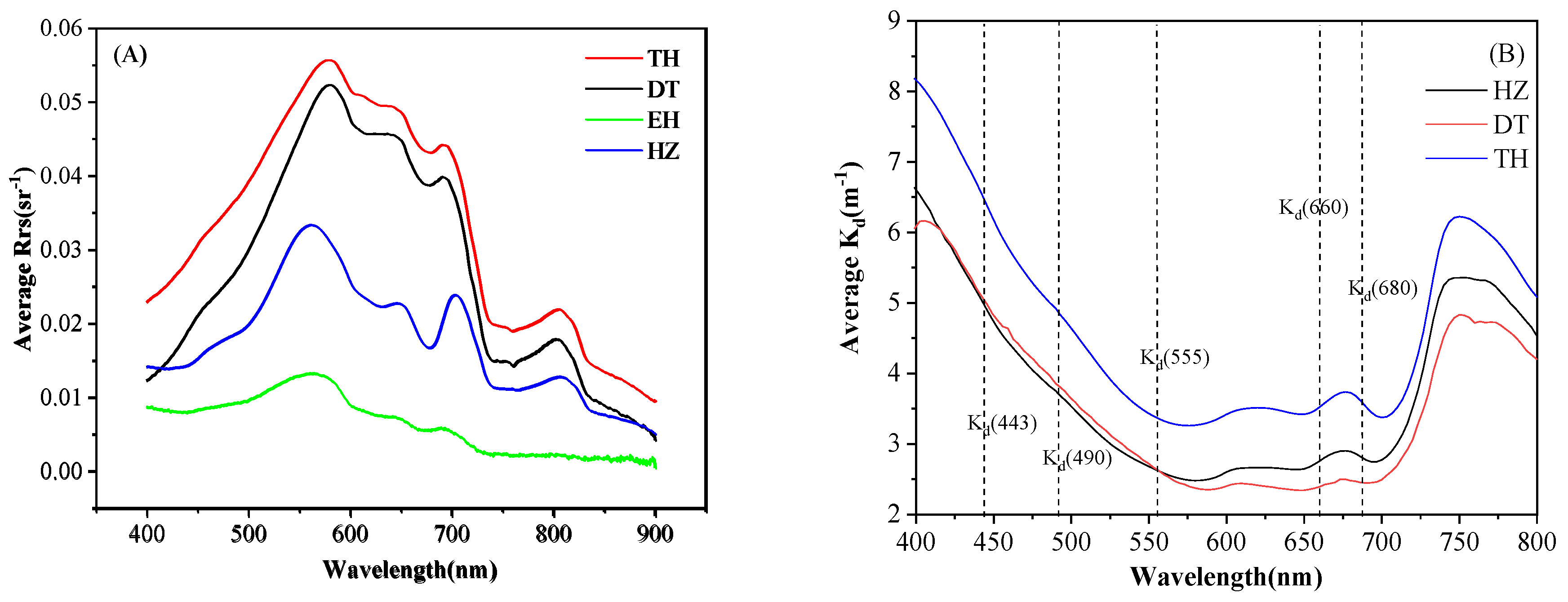
3.1. Biogeochemical and Optical Characterization

Table 2. Descriptive statistics from Lake Hongze (HZ), Lake Taihu (TH), Lake Dongting, and Lake Erhai (EH).

Parameters	Statistics	HZ(N = 87)	TH(N = 58)	DT(N = 40)	EH(N = 47)
Chla (μg/L)	Min–Max	1.39–149	9.23–301.93	2.79–52.08	7.27–34.34
	Aver ± SD	13.67 ± 19.5	57.44 ± 46.3	16.08 ± 12.4	14.74 ± 5.51
	CV(%)	142.64	80.61	77.61	37.36
TSM (mg/L)	Min–Max	7.18–193.33	8.66–96.47	3.75–200.53	1.96–7.5
	Aver ± SD	58.22 ± 31.77	33.16 ± 22.6	52.44 ± 46.5	3.91 ± 1.01
	CV(%)	54.57	68.15	88.62	25.82
ISM (mg/L)	Min–Max	5.45–174.16	4.22–79.41	1.65–182.93	0.15–4
	Aver ± SD	50.48 ± 29.28	19.68 ± 17.84	45.36 ± 44.16	2.89 ± 0.82
	CV(%)	58.01	90.66	97.35	66.77
OSM (mg/L)	Min–Max	1.23–35.07	3.44–59.85	2.1–19.46	1.83–5.3
	Aver ± SD	7.73 ± 4.59	13.47 ± 9.15	7.11 ± 3.76	2.89 ± 0.82
	CV(%)	59.37	67.91	52.93	28.61
ZSD (m)	Min-Max	0.15–0.8	0.15–1.0	0.15–1.05	0.9–2.48
	Aver ± SD	0.28 ± 0.13	0.43 ± 0.24	0.5 ± 0.25	1.56 ± 0.34
	CV(%)	72.43	56	51.3	22.37
OSM/TSM	Min–Max	0.03–0.47	0.16–0.81	0.05–0.61	0.03–0.53
	Aver ± SD	0.14 ± 0.07	0.46 ± 0.16	0.19 ± 0.12	0.27 ± 0.13
	CV(%)	49.46	36.16	63.57	47.64

Aver–average, SD–standard deviation, CV–coefficient of variation.

summarized the basic statistics of the field measured water quality parameters in Lake Hongze (HZ), Lake Taihu (TH), and Lake Dongting (DT). The parameters from these lakes showed a coefficient of variation (CV) between 17.36% and 142.64%, which indicated high dynamic ranges and substantial variability amongst the samples in the study areas. Although differences in the concentration of water parameters are present in these three lakes, they are all characterized by high turbidity.

In Lake Hongze, the maximum values of Chla, TSM, and Z_SD were more than 15 times larger than the minimum values. The Chla, TSM, and Z_SD were 1.39–149.32 μg/L, 7.18–193.33 mg/L, and 0.1–0.8 m, respectively. In Lake Hongze, the share of OSM in TSM is smaller than that of ISM, which demonstrated that ISM dominated the TSM in Lake Hongze. In Lake Taihu, the Chla, TSM, and Z_SD were 9.23–301.93 μg/L, 8.66–96.47 mg/L, and 0.14–1.1 mg/L, respectively. The maximum values of Chla, TSM and Z_SD were 32, 11, and 7 fold larger than the minimum values. The ratio of OSM to TSM (OSM / TSM > 0.5) indicates that suspended particulates in Lake Taihu are mainly dominated by organic suspended particulates. In Lake Dongting, the Chla, TSM and Z_SD were 2.79–52.08 μg/L, 3.75–200.53 mg/L and 0.15–1.05 mg/L, respectively. In Lake Erhai, the Chla, TSM and Z_SD were 7.27–34.34 μg/L, 1.96–7.5 mg/L, and 0.15–4 mg/L, respectively. Overall, Lake Hongze, Lake Taihu, Lake Dongting, and Lake Erhai showed high levels of suspended matter and Chla, but low Z_SD, which showed huge concentration differences with other inland waterbodies [4,33,34,35], indicating that Lake Hongze and Lake Taihu have the characteristics of highly turbid waters.

The average Rrs(λ) spectra in four lakes (HZ, DT, TH, and EH) had distinct characteristics, as shown in Figure 3A. Note that Lake Erhai has not field measured $K_d\left(\lambda \right)$ data used in this study. When compared with Lake Hongze and Lake Erhai, Lake Taihu and Lake Dongting have a higher spectral reflection curve due to the high intensity reflections. In addition, there is an obvious reflection peak and absorption trough appearing at 550 nm and 680 nm, respectively. Similar curve variations of $K_d\left(\lambda \right)$ were observed in Lake Taihu, Lake Dongting and Lake Hongze, all of which had a decreasing tendency from 400 to 570 nm and an increasing tendency from 700 to 750 nm Figure 3B. At the same time, the diffusion attenuation coefficient at 555 nm ($K_d\left(555\right)$) presents a minimum value within the visible domain (443–665 nm) rather than other bands in GOCI images.

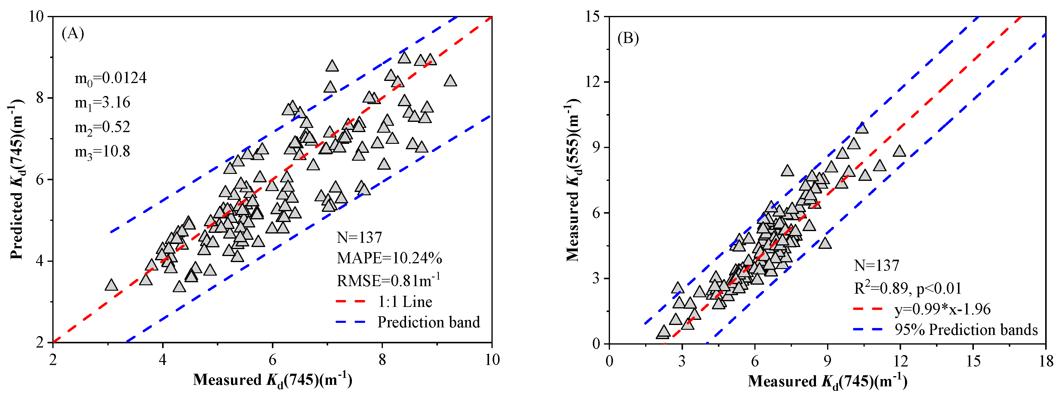
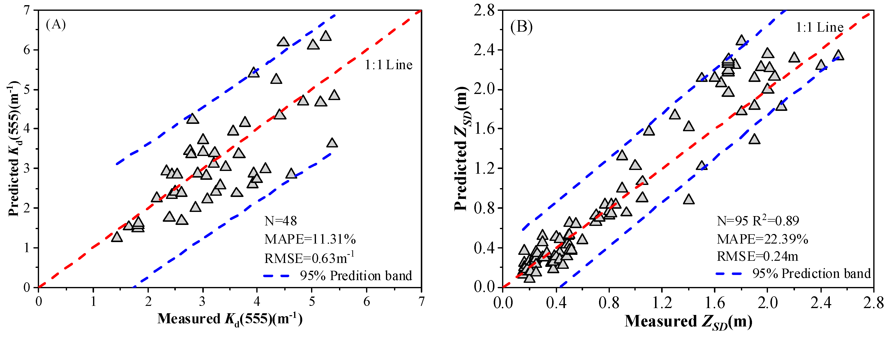
3.2. Algorithm Validation and Noise-Equivalent Z_SD

Although the model presented a significant improvement in the robustness to turbid water, comprehensive testing using in situ data that were obtained under various water conditions is still critical for algorithm validation and subsequent application to these extremely turbid waters. The remaining dataset (95 samples) was used to validate the semi-analytical algorithm of Z_SD. Note that only 48 validated samples have field measured $K_d\left(\lambda \right)$ data. The in-situ measured and corresponding retrieved values of $K_d\left(555\right)$ and Z_SD were distributed well along the 1:1 line (Figure 4). The MAPE and RMSE of match-up points between the measured and retrieved $K_d\left(555\right)$ were 11.31% and 0.63 m⁻¹, respectively (Figure 4A). This suggests that the modified steps in the new algorithm (step 3, 5, and 6) performed well with satisfactory accuracy and had great potential to further estimate the Z_SD in turbid lakes. The MAPE and RMSE of match-up points between the measured and retrieved Z_SD were 22.39% and 0.24 m, respectively (Figure 4B), which demonstrates that the performance of the semi-analytical algorithm of Z_SD had great potential for estimating Z_SD in satellite images.

Remote sensing of water clarity relies not only on validated algorithms for Z_SD, but also on the quality of remotely sensed imagery. Some previous studies [31,36] showed significant differences of imagery quality in the difference sensors between open sea and inland turbid waters, raising the question of whether GOCI imagery are suitable for the algorithm that we proposed for mapping Z_SD. Finally, the noise-equivalent Z_SD of 0.084 m was calculated based on our developed algorithm. When considering its well noise-equivalent Z_SD, GOCI imagery can be used for Z_SD estimation while using our developed algorithm in extremely turbid inland waters, such as Lake Taihu and Lake Hongze.

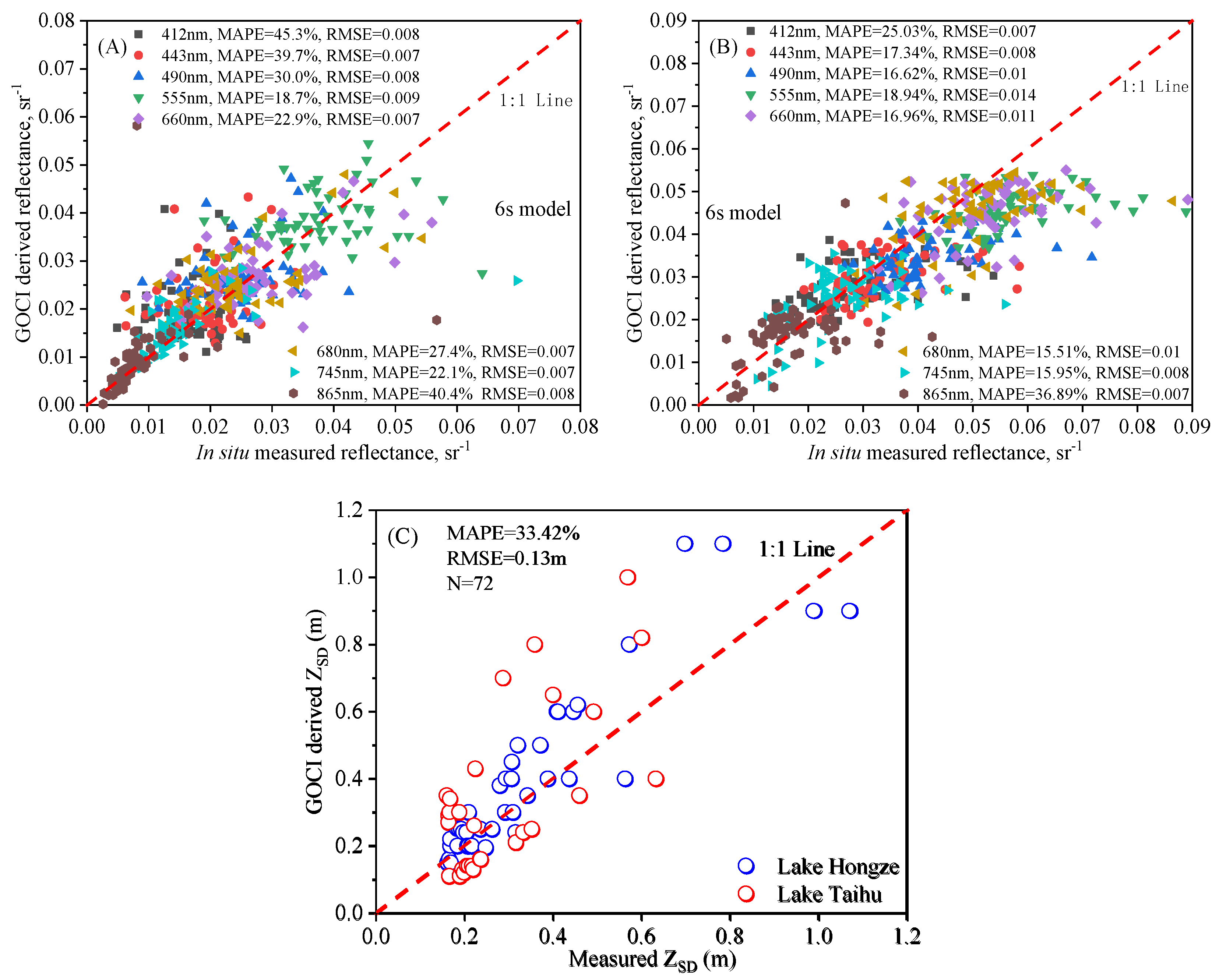
3.3. Atmospheric Correction Assessment by Synchronized Images

The performance of the 6S model mentioned in Section 2.3 and the Z_SD deriving algorithm were evaluated by comparing the GOCI-derived and the synchronized field measured Rrs at 443, 560, 665, 674, 709, and 754 nm (Figure 5), while the field measured reflectance obtained by ASD measurement were integrated while using the GOCI spectral response functions (SRF) to simulate the Rrs at the ground level. There are 42 synchronized in-situ samples in Lake Hongze and 30 samples in Lake Taihu.

For both turbid lakes, the MAPE values at 490, 555, 660, 680, and 745 nm were less than 30%, and poor performance of atmospheric correction at 412 nm was found (MAPE > 30%), which might be related to the characteristic that the spectrum is prone to saturation at the short blue wavelengths [37]. At the same time, poor performance existed at 865 nm with MAPE > 32% due to the high absorbing properties in NIR wavelengths for turbid water [38]. Overall, the GOCI-derived and field obtained Rrs(λ) were close to the 1:1 line. Given the superior performance of the 6S algorithm, it is reasonable to use it for atmospheric correction of GOCI data.

For the performance of Z_SDZ algorithm, the in situ measured Z_SD and the corresponding retrieved values were close to the 1:1 line (Figure 5C). The MAPE and RMSE for the validation of the developed models were 29.07% and 0.12 m, respectively. This suggests that our proposed retrieval models that were based on GOCI data performed well.

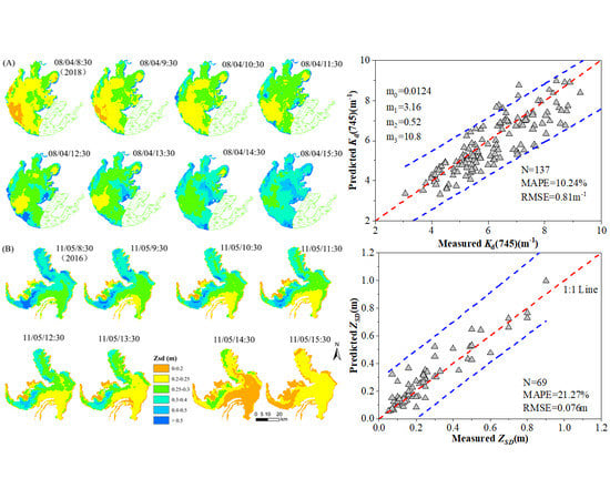
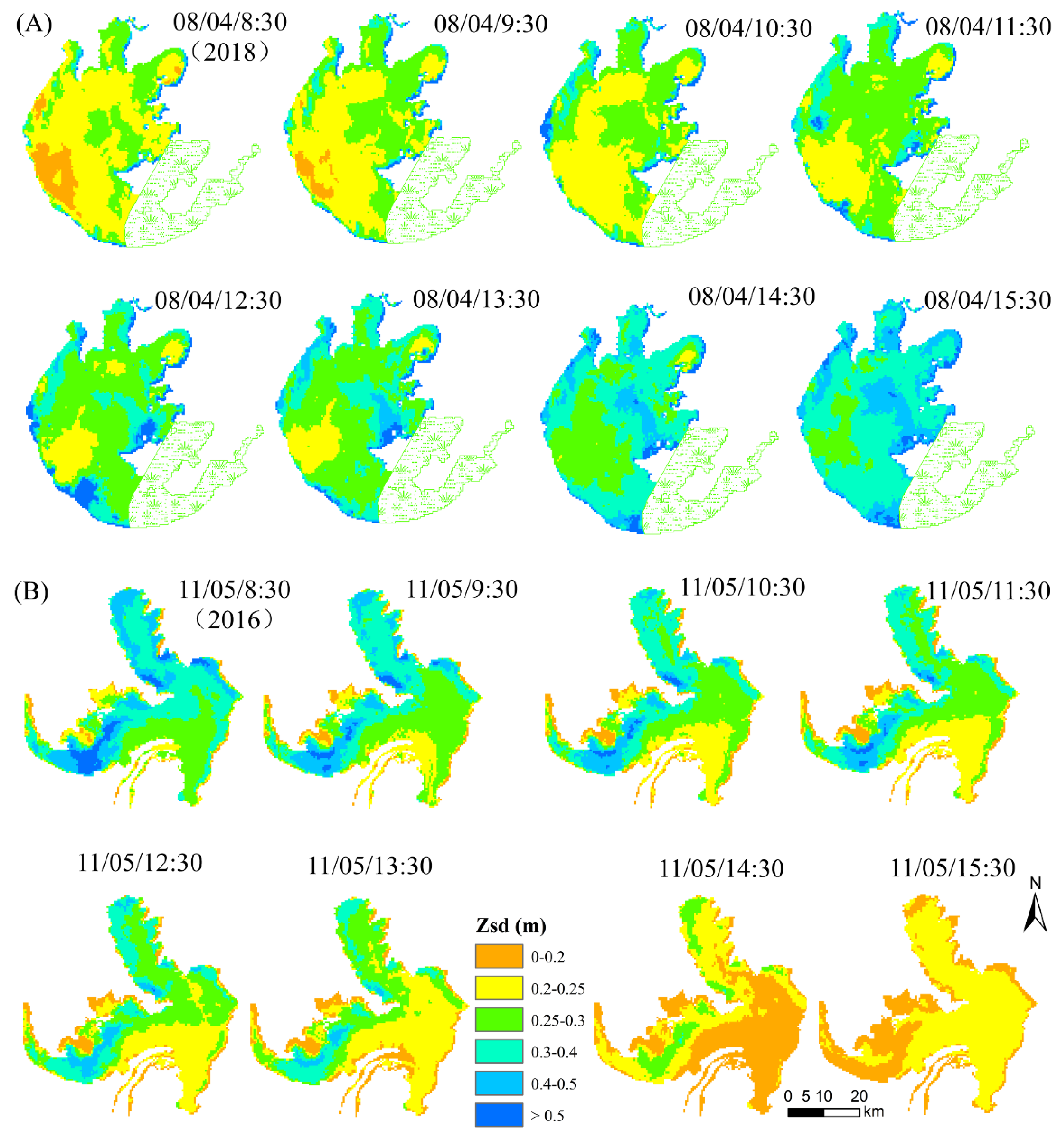
3.4. Mapping Z_SD from GOCI Based on Developed Algorithm

The GOCI Level-1B data, captured on, 4 August 2018 in Lake Taihu and 5 November 2016 in Lake Hongze, were used to estimate Z_SD based on our developed algorithm. The newly developed semi-analytical algorithm was applied to GOCI atmosphere corrected images in order to derive the hourly scale of Z_SD in Lake Taihu and Lake Hongze (Figure 6). The Z_SD retrieval results in the eastern part of Lake Taihu are not shown due to the impact of submerged vegetation and bottom reflectance. The hourly scale maps show the consecutive spatiotemporal dynamic characteristics of Z_SD in both Lake Taihu and Hongze with low Z_SD values within one day. Lake Taihu and Lake Hongze are shallow inland turbid waters, which are susceptible to environmental and anthropogenic factors, and they have significantly different characteristics from other inland waterbodies.

Significant spatiotemporal variability in Z_SD was present from 8:30 to 15:30 in Lake Taihu. The spatiotemporal distribution of Z_SD was significantly regulated by particulate suspended matter in Lake Taihu as a result of wind speed and wind direction [5,39]. The distribution of low Z_SD is mostly concentrated in the southwest areas of Taihu Lake, whereas high values were observed in central open zones and lake bays (such as Meiliang Bay, as shown in Figure 1). Sheltered conditions and large amounts of submerged aquatic vegetation, which maintain relatively high transparency due to the water filtration, wind-induced wave attenuation, and the inhibition of sediment resupension by aquatic vegetation characterize these areas [5,39]. In conclusion, wind conditions and submerged aquatic vegetation can both regulate the distribution of Z_SD in Lake Taihu. In addition, a key finding was that the Z_SD value of Lake Taihu shows a distinct increasing trend from 8:30 in the morning to 15:30 in the afternoon, which is probably due to the continued weakening of wind speed from morning to afternoon.

A different distribution pattern of Z_SD was observed in Lake Hongze than in Lake Taihu, which is, the transparency value showed a significant downward trend from 8:30 a.m. to 15:30 p.m. Temporally, the Z_SD in the eastern and northern part of Lake Hongze go through a process from high to low, whereas the Z_SD in the southwestern Lake remains low from 8:30 to 15:30. Spatially, the distribution of high Z_SD is concentrated in the north and west of Lake Hongze, whereas the low values were observed in the southern region, especially in the upstream riverine region (Figure 6B). The headwater of Huai River accounts for more than 70% of the annual mean incoming runoff of Lake Hongze; the vigorous movement of water is one of main factors for the low transparency in these areas [19].

4. Discussion

4.1. The Relationship between In-Situ Z_SD and Water Constituent Concentrations

In the present study, the field measured Z_SD values were low, with 0.15–0.8 m in Lake Hongze and 0.15 m–1.0 m in Lake Taihu, indicating that extreme turbidity characterizes these two lakes. These findings were similar to those found in other turbid inland lakes [40,41], as well as previous studies in Lake Taihu [42]. However, the Z_SD values in Lake Hongze and Lake Taihu are obviously lower than those for oceanic and coastal waters [10,11], and slightly turbid waters [4,6]. For example, the mean value of the field measured Z_SD in Lake Hongze is six times lower than that for Lake Qiandao [4].

Suspended particulate matter, phytoplankton, submerged vegetation, and the surface turbulence of the lake water affect Z_SD [5,43]. Among these, the concentrations of main optical components (such as Chl-a and TSM) and their relative contributions to Z_SD vary for different waters [4,5,8]. For example, in open marine waters, the optical properties are mainly dominated by phytoplankton and its attachments substantially contribute to the variability in Z_SD. In contrast, particulate sediment and debris may have a significant effect on water clarity in turbid lakes [5].

Robust positive correlation coefficients between Z_SD and TSM were found in both Lake Hongze and Lake Taihu (Figure 7A), indicating that Z_SD has a tight relationship with TSM; more than 60% of the Z_SD dynamic can be explained by the TSM in these two lakes. Relative higher correlation coefficients between Z_SD and ISM were also found in Lake Hongze (R² = 0.60, p < 0.01) and Lake Taihu (R² = 0.59, p < 0.01), whereas low values between Z_SD and OSM were in both lakes. Note that the coefficient in Lake Hongze (R² = 0.31, p < 0.01) is higher than that in Lake Taihu (R² = 0.08, p < 0.01), indicating that there are different water compositions between these two lakes. These results conclude that inorganic suspended matter (ISM), rather than organic suspended matter (OSM), plays an important role in water quality parameters that affects transparency. In addition, the relationships between field measured Z_SD and field measured Chla in both lakes were poor (Figure 7C,D).

The ratio of OSM/TSM is commonly used to indicate the relative quantity of ISM and OSM in water bodies. The mean values of OSM/TSM in Lake Hongze and Lake Taihu are 0.14 and 0.46, respectively, which suggests that inorganic suspended matter is dominant in Lake Hongze and Lake Taihu. This is different from other inland lakes (like Lake Chaohu and Lake Dianchi) that are dominated by organic suspended matter [44,45]. The low Z_SD values are characterized by high turbidity and high TSM. High TSM caused by sediment resuspension significantly decreased the water clarity [46]. Moreover, sediment resuspension can be induced by meteorological and hydrological events, such as rainstorms, strong winds, and human activities, such as sailing and trawling [47]. The intense water currents and sand mining activities in Lake Hongze cause sediment resuspension and reduce water transparency, especially in the estuarine part of the lake, according to the study by Lei et al. [20].

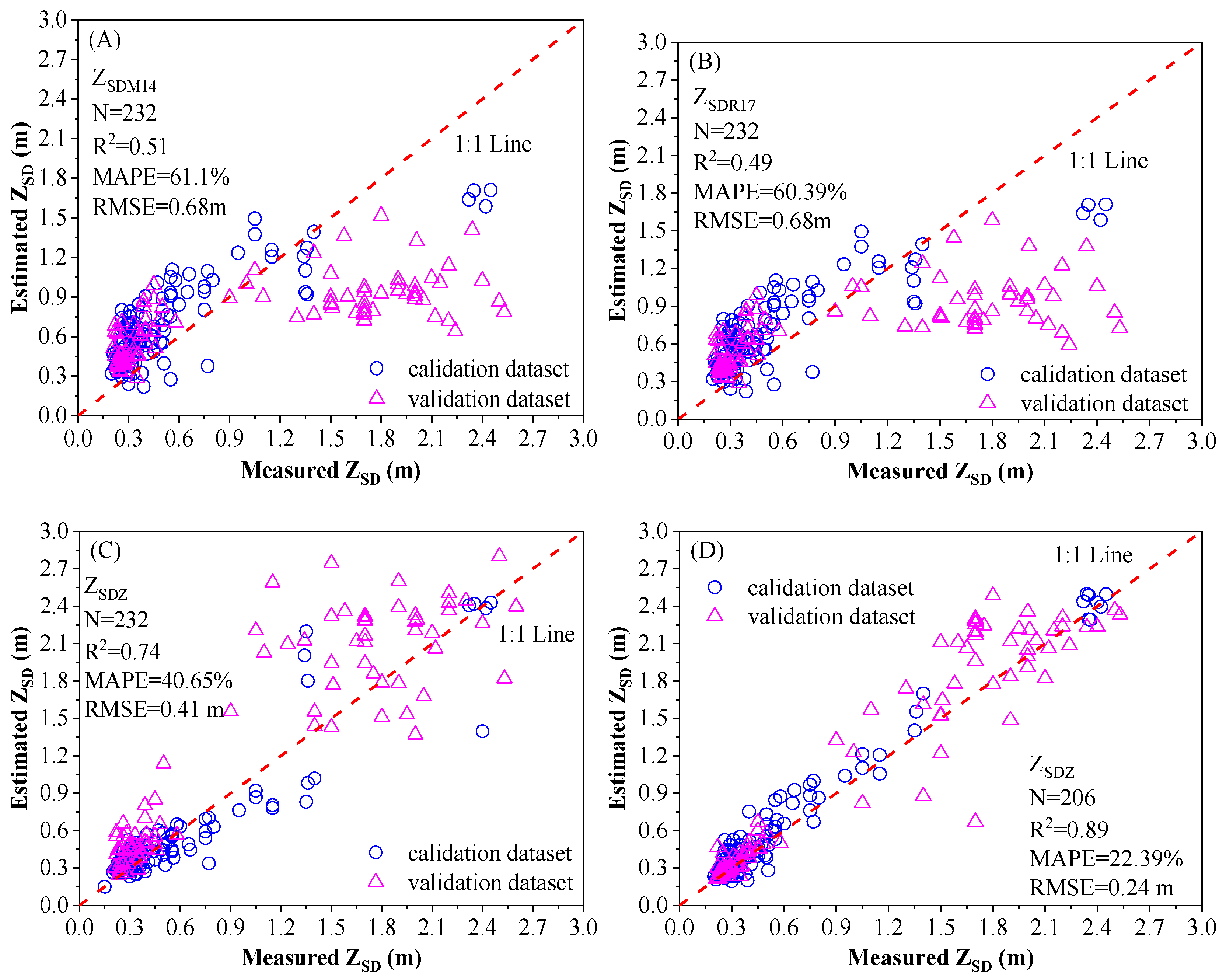
4.2. Comparison with the Exist Z_SD Algorithms for GOCI

An original and several modified algorithms for estimating Z_SD in slightly turbid or turbid waters have been proposed [6,11,12]. These algorithms were selected for comparison with our developed model in this study (

Table 3. Comparison of performance between the existing semi-analytical Z_SD models.

Models	Reference	R2	RMSE	MAPE
ZSDM14 (Model 1)	[6,49]	0.51	0.68 m	61.10%
ZSDR17 (Model 2)	[6]	0.56	0.68 m	60.39%
ZSDV6 (Model 3)	[10]	0.74	0.41 m	40.65%
ZSDZ (Model 4)	This study	0.89	0.24 m	22.39%

and Figure 8). Model 4 (Z_SDV6) was the original semi-analytical algorithm of Z_SD, and this model was developed and validated with large data covering inland, marine, and coastal waters [10]. Model 1 (denoted as Z_SDM14) and 2 (denoted as Z_SDR17) were developed by parameterizing and calibrating for application in highly turbid coastal and slightly turbid waters [6,48].

The results show the diverse performance of the different algorithms. Model 3 and 4 performed better than model 1 and 2, and the performance of Model 4 was best with relatively low MAPE (MAPE = 22.39%) and RMSE (RMSE = 0.24 m), but high R2 (R² = 0.89). Model 3 performed well for low Z_SD, but it had an overestimation effect for high Z_SD, which was consistent with a previous finding in slightly turbid waters [6]. Among the existing models, model 1 and 2 significantly underestimated Z_SD, which suggested that the original Z_SD algorithm that was proposed by Lee et al. [10] was more suitable than others in turbid inland waters. The results indicate that, although the three existing models can be used to estimate Z_SD in turbid inland waters, their performance was highly impacted by the local parameters and parameterization of the inherent optical properties, the new proposed model showed the best estimation effect.

4.3. Factors in the Z_SD Inversions

4.3.1. Model Parameterization

A suitable model is needed to estimate the total absorption and backscattering coefficients and further retrieve the water transparency (Z_SD) in turbid lakes. The values of Z_SD were underestimated or overestimated based on existing algorithms (Figure 6), which was probably due to these algorithms introducing larger uncertainty into the derived IOPs and further leading to the poorer performance of Z_SD in turbid inland waters. Lee et al. [12] noticed the underestimated IOPs using original QAA for turbid waters and concluded that the larger absorption effect of particulates at short wavelengths results in the weak accuracy of the model. Although several modified versions have been proposed for slightly turbid and coastal waters [6,48], the uncertainty analysis of semi-analytical algorithms for deriving Z_SD in extremely turbid lakes is seldom reported.

The uncertainty analysis that was carried out by previous studies [6,28] suggested that the reference wavelength shifted to longer wavelengths in turbid waterbodies that have low absorption but high scattering coefficients. Röttgers et al. [49] also found that the near infrared (NIR) absorption of particulates was approximately equal to the absorption of water in turbid waters. Liu et al. [50] noticed that selecting the appropriate NIR band as the reference wavelengths depends on varying types of turbid waters. In this study, the absorption in reference wavelength was assumed at 745 nm (step 3 in Table 1), which took into consideration that the absorption of pure water should dominate in this band. However, numerical difference was found between $a\left({\lambda }_0\right)$ and $a_{\mathrm{w}}\left({\lambda }_0\right)$ in step 3, which would propagate to the estimation of IOPs in step 3–6, and then to the estimation of Z_SD in step 7.

In step 2, g0 and g1 are both empirically constant and the optimized values can improve the estimation of the IOPs value. Ogashawara et al. [51] indicated that the derived u(λ) based on fixing the g0 and g1 values can result in an underestimation of a(λ) for different waters. The g0 = 0.089 and g1 = 0.1245 are suggested in the three versions of QAA (v4–6) for Case II waters [10,28]. Lee et al. [52] also demonstrated that g0 = 0.084 and g1 = 0.17 for higher scattering coastal waters and the same values are also applied in this study when considering the water properties of Lake Hongze and Lake Taihu. For $K_d\left({\lambda }_0\right)$ retrieval in step 5, the values of coefficients (m0~3) were also retuned while using the field measured datasets and the model brought the estimated $K_d\left(745\right)$ close to the field measured values (Figure 3A), indicating the necessity of parameter readjustment in our study.

4.3.2. Measurement Uncertainties

The uncertainty from field measured and satellite-derived Rrs(λ) also has a negative impact on the estimation of the IOPs and Z_SD. The measurement of spectral data followed the above-water measurement method in this study. It is worth noting that the water-leaving radiance was obtained by correcting the total radiance of the water surface ($L_t$) while using the coefficient of skylight reflectance ($r_{aw}$), which depended on the water surface conditions that are caused by wind conditions [21]. Zheng et al. [21] suggested that $r_{aw}$= 0.022 for calm conditions, 0.025 for < 5 m/s wind speed, and 0.026–0.028 for 10 m/s wind speed. According to field measured speed data that we collected, low wind speeds are dominant in Lake Hongze and Lake Taihu, and $r_{aw}$= 0.022 was applied in this study. However, the variation of $r_{aw}$ would result in a high variation of mean coefficient variance value (CV = ~50%) of Rrs at the spectral range of 400 to 800 nm [15], which definitely has a negative impact on the performance of Z_SD models. Moreover, although a reliable method was used to reduce sun glint and ensure the accurate measurement of reflectance, it is still possible for glint to remain. In addition, the inherent noise that is generated by the sensor is also an influencing factor.

In this study, the atmospheric correction was based on the 6S method to obtain the GOCI-derived Rrs. However, slight overcorrection of Rrs(745) and Rrs(555) were also found, which, as key input parameters, may introduce uncertainty into the derived IOPs and further lead to the poorer performance of Z_SD. The sensibility of using improved semi-analytical model of Z_SD for the input parameters (Rrs(745) and Rrs(555)) were analyzed, the result indicated that this model is highly sensitive to the atmospheric corrected GOCI-derived Rrs (Figure 9). Therefore, the retrieved IOPs rely on the accuracy of corrected Rrs directly, indicating that an excellent atmospheric correction model with high accuracy is necessary.

4.3.3. Limitation of Model in Retrieving Z_SD

For the Z_SDZ algorithm, one of the key steps (step 3 in Table 1) is to shift the reference wavelength to longer NIR band in order to satisfy an assumed condition that the $a_{\mathrm{w}}\left({\lambda }_0\right)$ is dominant in NIR wavelength. Additionally, the relatively high $R_{rs}\left({\lambda }_0\right)$ value in extremely turbid waters in NIR wavelength provides a higher signal-to-noise ratio to ensure the algorithm development. Conversely, for some slightly turbid waters or clear waters, a relatively low $R_{rs}\left({\lambda }_0\right)$ magnitude at longer NIR wavelength implies a low SNR, which might introduce large uncertainty to estimate $a\left({\lambda }_0\right)$. Although we do not have enough datasets to validate whether the developed algorithm can effectively estimate Z_SD in slightly turbid or clear waters, caution should be exercised in applying the newly developed algorithm to the above waters. One empirical step (step 5 in Table 1) was constructed based on field measured data that we collected, which is location dependent and may not be suitable to other waters. Therefore, when our algorithm is applied to other water bodies, it might be necessary to reconstruct similar empirical equations based on the optical properties of water.

The water quality and optical parameters of Lake Hongze and Lake Taihu have high variability, as presented in Table 2 and Figure 3. The Rrs, for example, has high variability of coefficient variance at 555 nm (CV = 54%), which is probably due to larger contribution of backscattering from particulates in extremely turbid water. Additionally, high variability of Chla (CV = 142.64%) in Lake Hongze and the ISM (CV = 90.66%) in Lake Taihu was observed. Obviously, high spatial dynamic of bio-optical properties in this study area limit the accuracy of Z_SD model. Therefore, for waterbodies with a high spatial dynamic of bio-optical properties, the retrieval of IOPs and the estimation of Z_SD may be compromised based on Z_SDZ algorithm.

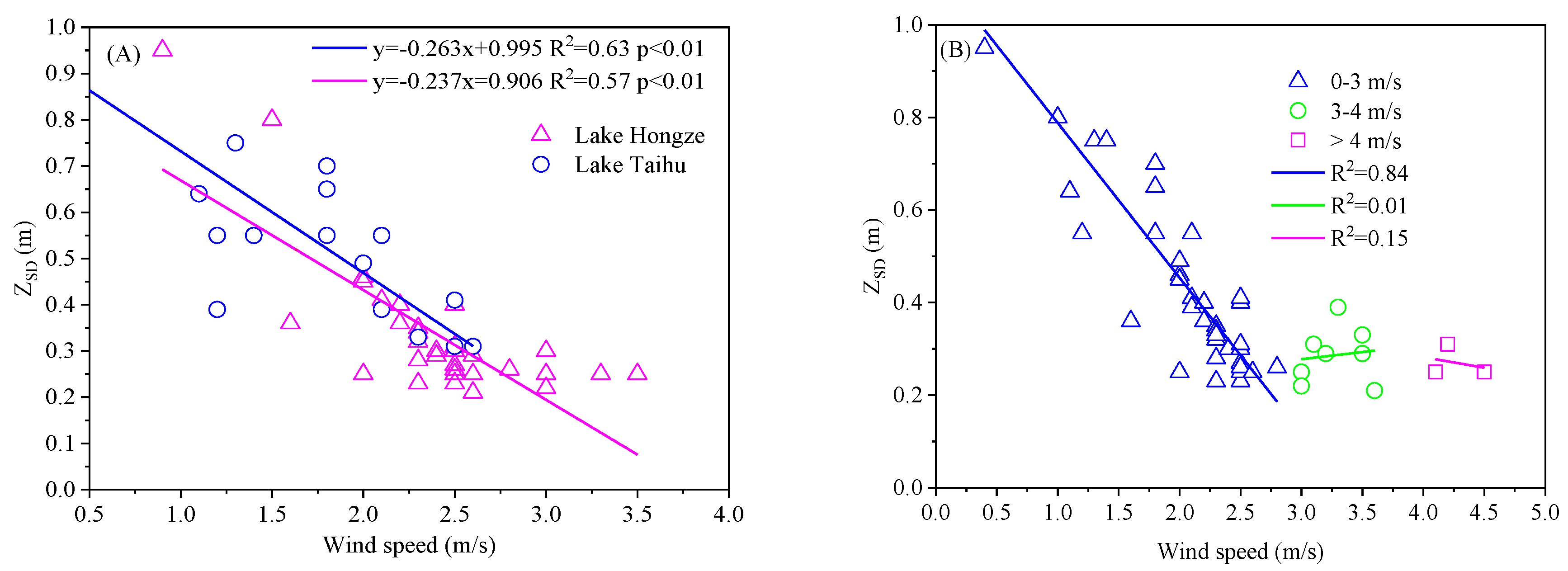
4.4. The Response of GOCI-Derived Z_SD to Wind Speed

Lake Hongze and Lake Taihu are characterized by shallow and turbid water, with an average depth of no more than 2 m, the wind forcing, river sediment discharge, and the short-term rainfall often lead to strong water mixing and suspension of particles [20,46]. This process results in an increase in TSM concentration, which then leads to weak light transmission and low water transparency. In addition, low wind speeds in enclosed areas often promote the growth of submerged aquatic vegetation with the functions of water filtration, water purification, and sediment resuspension reduction [5,47]. Figure 10 presents the hourly variation of GOCI-derived Z_SD and the corresponding wind speed. Strong relationships between GOCI-derived Z_SD and wind speed are found in both Lake Hongze (R² = 0.57, p < 0.01) and Lake Taihu (R² = 0.63, p < 0.01), and the Z_SD decreases with a reduction in wind speed, indicating that wind greatly affects the Z_SD.

To further understand the connection between Z_SD and wind speed, wind speed was divided into three levels: low (0–3 m/s), medium (3–4 m/s), and high (> 4 m/s), according to the intensity of the wind [53]. When the wind speed was low, the Z_SD varied from 0.08 m to 0.9 m with a mean value of 0.29 ± 0.21 m, and 84% of the variation of Z_SD can be explained by wind speed. However, when the wind condition was medium or high, the Z_SD ranged from 0.05 to 0.24 m with a mean value of 0.13 ± 0.05 m, and a weak relationship is observed between the wind speed and Z_SD (Figure 10B). The results indicate that low wind speeds are dominant in Lake Taihu and Lake Hongze, which is good for the growth of submerged aquatic vegetation. However, an increase in Z_SD is observed in both Lake Hongze and Lake Taihu, which might be related to anthropogenic activities [20,42].

5. Conclusions

An improved semi-analytical scheme (Z_SDZ) was developed to estimate water clarity in turbid waters. When compared with original Z_SDV6, the new method has three main extensions. Firstly, the reference wavelength for estimating $a\left({\lambda }_0\right)$ was relocated at 745 nm to reduce the adverse contribution from the optical components in extremely turbid waters. Second, four coefficients (m0 - m3) were modified based on field measured datasets to better estimate $K_d\left({\lambda }_0\right)$. Third, target $K_d\left(\lambda \right)$ was derived based on the good empirical relationship between $K_d\left(\lambda \right)$ and $K_d\left({\lambda }_0\right)$. The validation on a comprehensive field measured Z_SD dataset (69 samples) demonstrated that Z_SDZ improved the retrieval accuracy of Z_SD in turbid waters and outperformed the three existing semi-analytical schemes. The hourly variation patterns of Z_SD in Lake Hongze and Lake Taihu were also discovered after applying the Z_SDZ to GOCI data. A distinct difference was presented in the spatiotemporal distribution pattern of Z_SD between the two lakes. The transparency value showed a significant downward trend from 8:30 a.m. to 15:30 p.m. in Lake Hongze; conversely, a positive change in transparency was observed during the same time in Lake Taihu. Moreover, it has been found that wind is an important regulating factor in the spatiotemporal variation of Z_SD. Our findings suggest that our proposed algorithm that is based on GOCI imagery can be suitable for capturing and analyzing the hourly variation and the dynamic characteristics of transparency of turbid waterbodies in a good manner, providing an important source of information on monitoring and mitigating the adverse effects on ecosystems.

References

1. Bai, S.; Gao, J.; Sun, D.; Tian, M. Monitoring Water Transparency in Shallow and Eutrophic Lake Waters Based on GOCI Observations. Remote Sens. 2020, 12, 163. [Google Scholar] [CrossRef] [Green Version]
2. Jiang, D.; Matsushita, B.; Setiawan, F.; Vundo, A. An improved algorithm for estimating the Secchi disk depth from remote sensing data based on the new underwater visibility theory. ISPRS J. Photogramm. Remote Sens. 2019, 152, 13–23. [Google Scholar] [CrossRef]
3. Al Kaabi, M.; Zhao, J.; Ghedira, H. MODIS-Based Mapping of Secchi Disk Depth Using a Qualitative Algorithm in the Shallow Arabian Gulf. Remote Sens. 2016, 8, 423. [Google Scholar] [CrossRef] [Green Version]
4. Wu, Z.; Zhang, Y.; Zhou, Y.; Liu, M.; Shi, K.; Yu, Z. Seasonal-Spatial Distribution and Long-Term Variation of Transparency in Xin’anjiang Reservoir: Implications for Reservoir Management. Int. J. Environ. Res. Public Health 2015, 12, 9492–9507. [Google Scholar] [CrossRef] [PubMed]
5. Shi, K.; Zhang, Y.; Zhu, G.; Qin, B.; Pan, D. Deteriorating water clarity in shallow waters: Evidence from long term MODIS and in-situ observations. Int. J. Appl. Earth Obs. Geoinf. 2018, 68, 287–297. [Google Scholar] [CrossRef]
6. Rodrigues, T.; Alcântara, E.; Watanabe, F.; Imai, N. Retrieval of Secchi disk depth from a reservoir using a semi-analytical scheme. Remote Sens. Environ. 2017, 198, 213–228. [Google Scholar] [CrossRef] [Green Version]
7. Fukushima, T.; Matsushita, B.; Yang, W.; Jaelani, L.M. Semi-analytical prediction of Secchi depth transparency in Lake Kasumigaura using MERIS data. Limnology 2017, 19, 89–100. [Google Scholar] [CrossRef]
8. Binding, C.E.; Greenberg, T.A.; Watson, S.B.; Rastin, S.; Gould, J. Long term water clarity changes in North America’s Great Lakes from multi-sensor satellite observations. Limnol. Oceanogr. 2015, 60, 1976–1995. [Google Scholar] [CrossRef]
9. Preisendorfer, R.W. Secchi disk science: Visual optics of natural waters. Limnol. Oceanogr. 1986, 31, 909. [Google Scholar] [CrossRef] [Green Version]
10. Lee, Z.; Shang, S.; Hu, C.; Du, K.; Weidemann, A.; Hou, W.; Lin, J.; Lin, G. Secchi disk depth: A new theory and mechanistic model for underwater visibility. Remote Sens. Environ. 2015, 169, 139–149. [Google Scholar] [CrossRef] [Green Version]
11. Shang, S.; Lee, Z.; Shi, L.; Lin, G.; Wei, G.; Li, X. Changes in water clarity of the Bohai Sea: Observations from MODIS. Remote Sens. Environ. 2016, 186, 22–31. [Google Scholar] [CrossRef] [Green Version]
12. Lee, Z.; Shang, S.; Qi, L.; Yan, J.; Lin, G. A semi-analytical scheme to estimate Secchi-disk depth from Landsat-8 measurements. Remote Sens. Environ. 2016, 177, 101–106. [Google Scholar] [CrossRef]
13. Wang, Y.; Shen, F.; Sokoletsky, L.; Sun, X. Validation and Calibration of QAA Algorithm for CDOM Absorption Retrieval in the Changjiang (Yangtze) Estuarine and Coastal Waters. Remote Sens. 2017, 9, 1192. [Google Scholar] [CrossRef] [Green Version]
14. Grunert, B.K.; Mouw, C.B.; Ciochetto, A.B. Deriving inherent optical properties from decomposition of hyperspectral non-water absorption. Remote Sens. Environ. 2019, 225, 193–206. [Google Scholar] [CrossRef] [Green Version]
15. Xue, K.; Ma, R.; Duan, H.; Shen, M.; Boss, E.; Cao, Z. Inversion of inherent optical properties in optically complex waters using sentinel-3A/OLCI images: A case study using China’s three largest freshwater lakes. Remote Sens. Environ. 2019, 225, 328–346. [Google Scholar] [CrossRef]
16. Watanabe, F.; Mishra, D.R.; Astuti, I.; Rodrigues, T.; Alcântara, E.; Imai, N.N.; Barbosa, C. Parametrization and calibration of a quasi-analytical algorithm for tropical eutrophic waters. ISPRS J. Photogramm. Remote Sens. 2016, 121, 28–47. [Google Scholar] [CrossRef] [Green Version]
17. Shen, F.; Zhou, Y.; Peng, X.; Chen, Y. Satellite multi-sensor mapping of suspended particulate matter in turbid estuarine and coastal ocean, China. Int. J. Remote Sens. 2014, 35, 4173–4192. [Google Scholar] [CrossRef]
18. Lou, X.; Hu, C. Diurnal changes of a harmful algal bloom in the East China Sea: Observations from GOCI. Remote Sens. Environ. 2014, 140, 562–572. [Google Scholar] [CrossRef]
19. Lei, S.; Xu, J.; Li, Y.; Du, C.; Liu, G.; Zheng, Z.; Xu, Y.; Lyu, H.; Mu, M.; Miao, S.; et al. An approach for retrieval of horizontal and vertical distribution of total suspended matter concentration from GOCI data over Lake Hongze. Sci. Total Environ. 2019, 700, 134524. [Google Scholar] [CrossRef]
20. Lei, S.; Xu, J.; Li, Y.; Lyu, H.; Liu, G.; Zheng, Z.; Xu, Y.; Du, C.; Zeng, S.; Wang, H.; et al. Temporal and spatial distribution of Kd(490) and its response to precipitation and wind in lake Hongze based on MODIS data. Ecol. Indic. 2020, 108, 105684. [Google Scholar] [CrossRef]
21. Zheng, Z.; Ren, J.; Li, Y.; Huang, C.; Liu, G.; Du, C.; Lyu, H. Remote sensing of diffuse attenuation coefficient patterns from Landsat 8 OLI imagery of turbid inland waters: A case study of Dongting Lake. Sci. Total Environ. 2016, 573, 39–54. [Google Scholar] [CrossRef] [PubMed]
22. Xu, J.; Lei, S.; Bi, S.; Li, Y.; Lyu, H.; Xu, J.; Xu, X.; Mu, M.; Miao, S.; Zeng, S.; et al. Tracking spatio-temporal dynamics of POC sources in eutrophic lakes by remote sensing. Water Res. 2020, 168, 115162. [Google Scholar] [CrossRef] [PubMed]
23. Lei, S.; Wu, D.; Li, Y.; Wang, Q.; Huang, C.; Liu, G.; Zheng, Z.; Du, C.; Mu, M.; Xu, J.; et al. Remote sensing monitoring of the suspended particle size in Hongze Lake based on GF-1 data. Int. J. Remote Sens. 2018, 40, 3179–3203. [Google Scholar] [CrossRef]
24. Zhang, Y.; Liu, X.; Yin, Y.; Wang, M.; Qin, B. A simple optical model to estimate diffuse attenuation coefficient of photosynthetically active radiation in an extremely turbid lake from surface reflectance. Opt. Express 2012, 20, 20482–20493. [Google Scholar] [CrossRef]
25. Chen, S.-L.; Zhang, G.-A.; Yang, S.-L.; Shi, J.Z. Temporal variations of fine suspended sediment concentration in the Changjiang River estuary and adjacent coastal waters, China. J. Hydrol. 2006, 331, 137–145. [Google Scholar] [CrossRef]
26. Lee, Z.; Lubac, B.; Werdell, J.; Arnone, R. An update of the quasi-analytical algorithm (QAA_v5). Int. Ocean Color Group Softw. Rep. 2009, 1–9. [Google Scholar]
27. Budhiman, S.; Suhyb Salama, M.; Vekerdy, Z.; Verhoef, W. Deriving optical properties of Mahakam Delta coastal waters, Indonesia using in situ measurements and ocean color model inversion. ISPRS J. Photogramm. Remote Sens. 2012, 68, 157–169. [Google Scholar] [CrossRef]
28. Lee, Z.; Ahn, Y.H.; Mobley, C.; Arnone, R. Removal of surface-reflected light for the measurement of remote-sensing reflectance from an above-surface platform. Opt. Express 2010, 18, 26313–26324. [Google Scholar] [CrossRef]
29. Morel, A.; Maritorena, S. Bio-optical properties of oceanic waters: A reappraisal. J. Geophys. Res. Ocean. 2001, 106, 7163–7180. [Google Scholar] [CrossRef] [Green Version]
30. Lee, Z.; Hu, C.; Shang, S.; Du, K.; Lewis, M.; Arnone, R.; Brewin, R. Penetration of UV-visible solar radiation in the global oceans: Insights from ocean color remote sensing. J. Geophys. Res. Ocean. 2013, 118, 4241–4255. [Google Scholar] [CrossRef] [Green Version]
31. Vanhellemont, Q.; Ruddick, K. Turbid wakes associated with offshore wind turbines observed with Landsat 8. Remote Sens. Environ. 2014, 145, 105–115. [Google Scholar] [CrossRef] [Green Version]
32. Ryu, J.-H.; Han, H.-J.; Cho, S.; Park, Y.-J.; Ahn, Y.-H. Overview of geostationary ocean color imager (GOCI) and GOCI data processing system (GDPS). Ocean. Sci. J. 2012, 47, 223–233. [Google Scholar] [CrossRef]
33. Zhang, Y.; Zhang, Y.; Shi, K.; Zha, Y.; Zhou, Y.; Liu, M. A Landsat 8 OLI-Based, Semianalytical Model for Estimating the Total Suspended Matter Concentration in the Slightly Turbid Xin’anjiang Reservoir (China). IEEE J. Sel. Top. Appl. Earth Obs. Remote Sens. 2016, 9, 398–413. [Google Scholar] [CrossRef]
34. Tang, X.; Wu, M.; Li, R. Phosphorus distribution and bioavailability dynamics in the mainstream water and surface sediment of the Three Gorges Reservoir between 2003 and 2010. Water Res. 2018, 145, 321–331. [Google Scholar] [CrossRef] [PubMed]
35. Volpe, V.; Silvestri, S.; Marani, M. Remote sensing retrieval of suspended sediment concentration in shallow waters. Remote Sens. Environ. 2011, 115, 44–54. [Google Scholar] [CrossRef]
36. Ren, J.; Zheng, Z.; Li, Y.; Lv, G.; Wang, Q.; Lyu, H.; Huang, C.; Liu, G.; Du, C.; Mu, M.; et al. Remote observation of water clarity patterns in Three Gorges Reservoir and Dongting Lake of China and their probable linkage to the Three Gorges Dam based on Landsat 8 imagery. Sci. Total Environ. 2018, 625, 1554–1566. [Google Scholar] [CrossRef] [PubMed]
37. Wang, M.H.; Shi, W.; Jiang, L.D. Atmospheric correction using near-infrared bands for satellite ocean color data processing in the turbid western Pacific region. Opt. Express 2012, 20, 741–753. [Google Scholar] [CrossRef]
38. Le, C.; Li, Y.; Zha, Y.; Sun, D.; Huang, C.; Lu, H. A four-band semi-analytical model for estimating chlorophyll a in highly turbid lakes: The case of Taihu Lake, China. Remote Sens. Environ. 2009, 113, 1175–1182. [Google Scholar] [CrossRef]
39. Zhang, Y.L.; Shi, K.; Liu, J.J.; Deng, J.M.; Qin, B.Q.; Zhu, G.W.; Zhou, Y.Q. Meteorological and hydrological conditions driving the formation and disappearance of black blooms, an ecological disaster phenomena of eutrophication and algal blooms. Sci. Total Environ. 2016, 569, 1517–1529. [Google Scholar] [CrossRef]
40. Arst, H.; Nõges, T.; Nõges, P.; Paavel, B. Relations of phytoplankton in situ primary production, chlorophyll concentration and underwater irradiance in turbid lakes. Hydrobiologia 2008, 599, 169–176. [Google Scholar] [CrossRef]
41. Liu, J.; Sun, D.; Zhang, Y.; Li, Y. Pre-classification improves relationships between water clarity, light attenuation, and suspended particulates in turbid inland waters. Hydrobiologia 2013, 711, 71–86. [Google Scholar] [CrossRef]
42. Shi, K.; Zhang, Y.; Liu, X.; Wang, M.; Qin, B. Remote sensing of diffuse attenuation coefficient of photosynthetically active radiation in Lake Taihu using MERIS data. Remote Sens. Environ. 2014, 140, 365–377. [Google Scholar] [CrossRef]
43. Feng, L.; Hou, X.; Zheng, Y. Monitoring and understanding the water transparency changes of fifty large lakes on the Yangtze Plain based on long-term MODIS observations. Remote Sens. Environ. 2019, 221, 675–686. [Google Scholar] [CrossRef]
44. Miao, S.; Lyu, H.; Wang, Q.; Li, Y.; Wu, Z.; Du, C.; Xu, J.; Bi, S.; Mu, M.; Lei, S. Estimation of terrestrial humic-like substances in inland lakes based on the optical and fluorescence characteristics of chromophoric dissolved organic matter (CDOM) using OLCI images. Ecol. Indic. 2019, 101, 399–409. [Google Scholar] [CrossRef]
45. Wu, Y.; Li, L.; Gan, N.; Zheng, L.; Ma, H.; Shan, K.; Liu, J.; Xiao, B.; Song, L. Seasonal dynamics of water bloom-forming Microcystis morphospecies and the associated extracellular microcystin concentrations in large, shallow, eutrophic Dianchi Lake. J. Environ. Sci. (China) 2014, 26, 1921–1929. [Google Scholar] [CrossRef]
46. Shi, K.; Zhang, Y.; Zhu, G.; Liu, X.; Zhou, Y.; Xu, H.; Qin, B.; Liu, G.; Li, Y. Long-term remote monitoring of total suspended matter concentration in Lake Taihu using 250m MODIS-Aqua data. Remote Sens. Environ. 2015, 164, 43–56. [Google Scholar] [CrossRef]
47. Liu, X.; Zhang, Y.; Yin, Y.; Wang, M.; Qin, B. Wind and submerged aquatic vegetation influence bio-optical properties in large shallow Lake Taihu, China. J. Geophys. Res. Biogeosciences 2013, 118, 713–727. [Google Scholar] [CrossRef]
48. Mishra, S.; Mishra, D.R.; Lee, Z. Bio-Optical Inversion in Highly Turbid and Cyanobacteria-Dominated Waters. IEEE Trans. Geosci. Remote Sens. 2014, 52, 375–388. [Google Scholar] [CrossRef]
49. Röttgers, R.; Dupouy, C.; Taylor, B.B.; Bracher, A.; Woźniak, S.B. Mass-specific light absorption coefficients of natural aquatic particles in the near-infrared spectral region. Limnol. Oceanogr. 2014, 59, 1449–1460. Available online: https://aslopubs.onlinelibrary.wiley.com/doi/abs/10.4319/lo.2014.59.5.1449 (accessed on 18 March 2020). [CrossRef] [Green Version]
50. Liu, G.; Li, L.; Song, K.; Li, Y.; Lyu, H.; Wen, Z.; Fang, C.; Bi, S.; Sun, X.; Wang, Z.; et al. An OLCI-based algorithm for semi-empirically partitioning absorption coefficient and estimating chlorophyll a concentration in various turbid case-2 waters. Remote Sens. Environ. 2020, 239, 111648. [Google Scholar] [CrossRef]
51. Ogashawara, I.; Mishra, D.R.; Nascimento, R.F.F.; Alcântara, E.H.; Kampel, M.; Stech, J.L. Re-parameterization of a quasi-analytical algorithm for colored dissolved organic matter dominant inland waters. Int. J. Appl. Earth Obs. Geoinf. 2016, 53, 128–145. [Google Scholar] [CrossRef] [Green Version]
52. Lee, Z.; Carder, K.L.; Mobley, C.D.; Steward, R.G.; Patch, J.S. Hyperspectral remote sensing for shallow waters. 2. Deriving bottom depths and water properties by optimization. Appl. Opt. 1999, 38, 3831–3843. [Google Scholar] [CrossRef] [PubMed] [Green Version]
53. Huang, C.; Shi, K.; Yang, H.; Li, Y.; Zhu, A.X.; Sun, D.; Xu, L.; Zou, J.; Chen, X. Satellite observation of hourly dynamic characteristics of algae with Geostationary Ocean Color Imager (GOCI) data in Lake Taihu. Remote Sens. Environ. 2015, 159, 278–287. [Google Scholar] [CrossRef]
Figure 1. The location of Lake Hongze (B), Lake Dongting (C), Lake Taihu (D), and Lake Erhai (E) in China (A). The symbols represent the sampling date in year-month forma.
Remotesensing 12 01516 g001
Figure 2. Comparison between measured and the model derived values of Kd(745) (A). The in-situ relationships between Kd(745) and Kd(555) (B).
Remotesensing 12 01516 g002
Figure 3. Average Rrs (A) and Kd (B) in Lake Hongze (HZ), Lake Taihu (TH), Lake Dongting (DT), and Lake Erhai (EH), respectively. The K d ( 555 ) is the minimum K d value within the visible domain for GOCI (B).
Remotesensing 12 01516 g003
Figure 4. Validation of the K d ( 555 ) (A) and ZSD (B) between the measured and predicted values. Applicability verification of the new algorithm in Lake Dongting.
Remotesensing 12 01516 g004
Figure 5. The field measured reflectance corresponded to the Geostationary Ocean Color Imager (GOCI) bands for Lake Taihu (A) and Lake Hongze (B). The performance of new algorithm based on synchronized images (C).
Remotesensing 12 01516 g005
Figure 6. Hourly variations of GOCI-derived ZSD based on ZSDZ model in Lake Taihu (A) and Lake Hongze (B). The retrieval results of ZSD in the eastern part of Lake Taihu are not shown due to the dense distribution of aquatic vegetation (see Figure 1).
Remotesensing 12 01516 g006
Figure 7. The relationship between measured ZSD and measured water quality parameters in Lake Hongze and Taihu: (A) total suspended matter (TSM), (B) inorganic suspended matter (ISM), (C) organic suspended matter (OSM), and (D) Chla.
Remotesensing 12 01516 g007
Figure 8. Comparison of the measured and derived ZSD of the four Models. (A) ZSDM14, (B) ZSDR17, and (C) ZSDV6 were provided by previous studies, (D) ZSDZ is provided by this study.
Remotesensing 12 01516 g008
Figure 9. Variation of mean absolute square percentage error (MAPE) for ZSD, derived from the errors introduced by atmospheric correction.
Remotesensing 12 01516 g009
Figure 10. The relationship between ZSD and wind speed (A) and scatterplot of different levels of wind speed and ZSD (B).
Remotesensing 12 01516 g010