Comparison of Statistical Modelling Approaches for Estimating Tropical Forest Aboveground Biomass Stock and Reporting Their Changes in Low-Intensity Logging Areas Using Multi-Temporal LiDAR Data

Abstract

Accurately quantifying forest aboveground biomass (AGB) is one of the most significant challenges in remote sensing, and is critical for understanding global carbon sequestration. Here, we evaluate the effectiveness of airborne LiDAR (Light Detection and Ranging) for monitoring AGB stocks and change (ΔAGB) in a selectively logged tropical forest in eastern Amazonia. Specifically, we compare results from a suite of different modelling methods with extensive field data. The calibration AGB values were derived from 85 square field plots sized 50 × 50 m field plots established in 2014 and which were estimated using airborne LiDAR data acquired in 2012, 2014, and 2017. LiDAR-derived metrics were selected based upon Principal Component Analysis (PCA) and used to estimate AGB stock and change. The statistical approaches were: ordinary least squares regression (OLS), and nine machine learning approaches: random forest (RF), several variations of k-nearest neighbour (k-NN), support vector machine (SVM), and artificial neural networks (ANN). Leave-one-out cross-validation (LOOCV) was used to compare performance based upon root mean square error (RMSE) and mean difference (MD). The results show that OLS had the best performance with an RMSE of 46.94 Mg/ha (19.7%) and R² = 0.70. RF, SVM, and ANN were adequate, and all approaches showed RMSE ≤54.48 Mg/ha (22.89%). Models derived from k-NN variations all showed RMSE ≥64.61 Mg/ha (27.09%). The OLS model was thus selected to map AGB across the time-series. The mean (±sd—standard deviation) predicted AGB stock at the landscape level was 229.10 (±232.13) Mg/ha in 2012, 258.18 (±106.53) in 2014, and 240.34 (sd ± 177.00) Mg/ha in 2017, showing the effect of forest growth in the first period and logging in the second period. In most cases, unlogged areas showed higher AGB stocks than logged areas. Our methods showed an increase in AGB in unlogged areas and detected small changes from reduced-impact logging (RIL) activities occurring after 2012. We also detected that the AGB increase in areas logged before 2012 was higher than in unlogged areas. Based on our findings, we expect our study could serve as a basis for programs such as REDD+ and assist in detecting and understanding AGB changes caused by selective logging activities in tropical forests.

1. Introduction

Tropical forests have been receiving increasing attention from scientists in the past couple of decades due to their significant contribution to the global carbon cycle. Forests by sequestering and storing great quantities of carbon act as natural ‘brakes’ on global climate change [1,2]. The Amazon rainforest is notable as the largest continuous area of tropical forest covering approximately 400 million hectares. Given its size, the volumes of carbon dioxide that it can emit and sequester are significant; it stores one-fifth of the total carbon in global terrestrial vegetation and is the largest carbon reservoir in the form of biomass [3,4].

Forest stand development and mortality are subject to natural and anthropogenic disturbances that alter carbon fluxes over time [5,6]. Consequently, economic incentives such as REDD+ exist to alter fluxes in favour of sequestration in forests; and depend on reliable monitoring, reporting, and verification (MRV) protocols [7]. Owing to the potential of tropical forests for sequestration, especially in comparison to other terrestrial ecosystems, an accurate estimate of the forest structure and biomass is necessary to better understand the global carbon cycle [8,9]. However, monitoring in tropical regions is a resource-intensive challenge resulting in infrequent and limited field surveys [10]. Thus, there is a need for reliable LiDAR-based AGB models, an area that is still developing.

Selective logging has been an important activity affecting land use [11] and modifying carbon fluxes within the Amazon, and can degrade the forest environment if logging exceeds the sustainable forest yield [12]. Consequently, reduced impact logging (RIL) techniques are being introduced to permit sustainable resource use of the Amazonian forest. RIL involves intensive planning and monitoring techniques, such as mapping and tree inventories, to minimize negative environmental impacts. It has been shown that well-planned logging can allow close to full recovery of carbon stocks [13,14].

Forest management, REDD+ MRV, and carbon cycle modelling all rely upon accurate estimates of forest aboveground biomass (AGB) stocks and their changes over time [15]. Previous studies have aimed at improving the accuracy of AGB estimation and forest inventory from LiDAR in regional and national level MRV systems such as those for REDD+ programs [16]. Such studies seek to adhere to the common interpretation of the IPCC guidelines stating that the uncertainty of the AGB should not be greater than 20% of the mean [17]. Airborne LiDAR data collection has become recognised in several forest ecosystems as the most reliable technique for estimating AGB [17,18,19]. LiDAR can be used to observe and facilitate the study of biomass carbon change at multiple scales [20], and to observe the impact of activities such as selective logging [15,21]. Research on the application of modelling methods for identifying these low-intensity logging practices using LiDAR is currently at an infant stage, though it is gaining momentum [22].

AGB can be estimated from LiDAR-derived attributes using a variety of statistical modeling approaches ranging from linear regression techniques to the state-of-art non-parametric methods such as Random Forest (RF), k-Nearest neighbour (k-NN), and Support Vector Machine (SVM), each depending on the underlying assumptions and complexities [16,23,24,25]. Additionally, a recent study by Shao et al. [26] on temperate hardwood forests highlighted the applicability of employing multiplicative nonlinear regression models for estimating AGB. In this case, the authors were able to leverage information on soil-based site productivity classes along with LiDAR-derived metrics to build an optimized model that could account for the variations in site productivity; including an index of site productivity which enhanced their model’s ability to explain the overall variability by 14%.

In recent years, there have been a number of studies focused on comparing the accuracy and precision of multiple machine learning approaches estimating biomass. For instance, Domingo et al. [27] performed a comparison of multiple linear regression model (MLR) with four non-parametric models—namely SVM, RF, locally weighted linear regression (LWLR), and a linear model with a minimum length principle (MDL)—to estimate total biomass (tree and shrub biomass fractions) in Pinus halepensis Miller forest stands using low-density LiDAR and field data. MLR was found to outperform other nonparametric methods in terms of RMSE (15.14 tons/ha) and bias (0.01) values, though no statistically significant differences existed between the methods considered. Similarly, Domingo et al. [28], compared the performance of nine regression models in quantifying biomass losses and CO₂ emissions due to combustion in an Aleppo pine forest using LiDAR data. Here too, the best model for pre-fire AGB estimation was found to be MLR, and no significant statistical differences were observed among the high performing models. Latifi et al. [29] on the other hand, made use of a wide range of forest variables extracted from multiple remotely sensed data, such as orthorectified colour infrared (CIR) images, medium-resolution Thematic Mapper (TM) imagery, and high-density normalized LiDAR point clouds, for estimating the total volume and biomass in a mixed temperate forest landscape. When comparing the performance of various plot-level nonparametric predictions, which comprised of three distance measures of Euclidean, Mahalanobis, and Most Similar Neighbour, as well as RF, and multiple remotely sensed datasets, the authors showed the superior predictive capability of LiDAR-based metrics and RF combination. Application of evolutionary genetic algorithms was also tested to prune the original high dimensional dataset and improve the performance of modeling techniques; however, intercorrelation related issues proved to be a major hurdle causing unstable results during multiple runs. Meanwhile, Gagliasso et al. [30], on examination of the predictive performance of linear regression, geographic weighted regression (GWR), gradient nearest neighbor (GNN), most similar neighbor (MSN), random forest imputation, and k-nearest neighbor (k-nn), observed that the k-nn (k = 5) had the lowest RMSE and least amount of bias while predicting biomass across 19,000 acres on the Malheur National Forest. Notwithstanding the ever-increasing interest in modeling paradigms, comparative modeling studies for AGB change prediction in selectively logged tropical forests remains nominal.

Even though airborne LiDAR can facilitate spatially explicit and timely estimates of tropical forest structure, trade-offs still exist between modeling techniques and AGB stocks, and AGB change estimations. For instance, it is unclear how much the models can be simplified and still maintain an adequate level of accuracy for AGB stocks estimation, and through the differences between estimates, report its AGB change in tropical forests. Thus, in this study, we aimed to estimate AGB stock and report the changes at the plot and landscape levels using multi-temporal LiDAR data for a selectively logged tropical forest in Amazonia, Brazil. Specifically, we compared nine machine learning approaches to traditional linear regression with the following objectives included in the scope of this study:

(i)

Evaluate the performance of ordinary least squares (OLS) regression modelling and nine machine learning algorithms: random forest (RF), several variations of k-nearest neighbour (k-NN), support vector machine (SVM), and artificial neural networks (ANN)

(ii)

Estimate AGB stocks and report AGB change at the landscape level using the best model from the previous step and multi-temporal LiDAR datasets.

2. Materials and Methods

2.1. Study Area

This study was conducted at Fazenda Cauaxi in Pará state, Brazil (Figure 1). The state of Pará is in the eastern Amazon, where logging and forest clearing for the purposes of land-use conversion and the gathering of fuelwood have been essential to the local economy of the study area for decades. The local climate is tropical humid, and the average total annual precipitation is approximately 2200 mm [31]. The predominant vegetation is Ombrophilous Dense Forest, also called terra firme (upland), with a mean upper canopy height of 30–40 m and scattered emergent trees up to 50 m tall [32]. Terra Firme literally means “firm earth” and refers to a rainforest that is not inundated by flooded rivers. This forest is noticeably taller and very diverse (> 400 species/hectare in some areas). According to the Brazilian system [33], the soils are mainly classified as dystrophic yellow latosols. The soils have low fertility due to the low reserve of nutrients such as calcium, magnesium, potassium, phosphorus, and nitrogen, in addition to high saturation by aluminum. The topography is mainly flat to mildly undulating [34] with the height above sea level in the study area ranging from 74 to 150 m [35].

2.2. Field Data

In 2014, the field dataset was collected across 85 plots of 50 × 50 m (0.25 ha) spaced at 100 m intervals along transects distributed across areas with logging within the study area (Figure 1b). Plot corners were registered using differential GNSS (GeoXH6000, Trimble Navigation, Ltd.; Dayton, OH, USA) [15]. Within each plot, sub-plots demarcated along one side of the plot had dimensions of 5 m × 50 m (250 m²). Only the trees within each plot with a diameter at 1.3 m breast height (dbh; cm) exceeding or equal to 35 cm were measured, whereas within the subplot’s trees with a dbh within the range 35 cm and 10 cm inclusive were measured. The AGB of each individual tree (agb; kg) was calculated using an allometric equation developed by Chave et al. [36], Equation (1):

$$agb=\exp \left[-1.803-0.976\mathrm{E}+0.976\ln \left(\rho \right)+2.673\ln \left(dbh\right)-0.0299\left[\ln \left(dbh\right)\right]²\right)]$$

(1)

where $\rho$ is the wood density (g/cm³) per species, which is derived from a published database [36]; E is a compounded measure of environmental stresses—such as variability in temperature and precipitation—which improves estimation when field measurements of tree height are not available. For this, we retrieved a value of E = −0.104 for the location of this study area. Total live AGB (Mg/ha) was calculated by aggregation of individual tree biomass values and using plot appropriate hectare expansion factors.

Table 1. Summary of input data (dbh and aboveground biomass - AGB) at the sample plots.

Attributes	Min	Max	Mean	sd
dbh (cm)	10	186.00	32.70	20.16
ρ (g/cm3)	0.26	0.99	0.73	0.14
AGB (kg·tree−1)	22.46	73.70	18.04	36.84
AGB ( Mg·ha−1)	65.34	525.79	238.11	86.48

presents a summary of the input data (dbh and AGB) in 2014, which were used for statistical analysis.

Figure 2 illustrates the research process that has been designed for estimating AGB stocks and AGB change using LiDAR data and statistical modeling approaches.

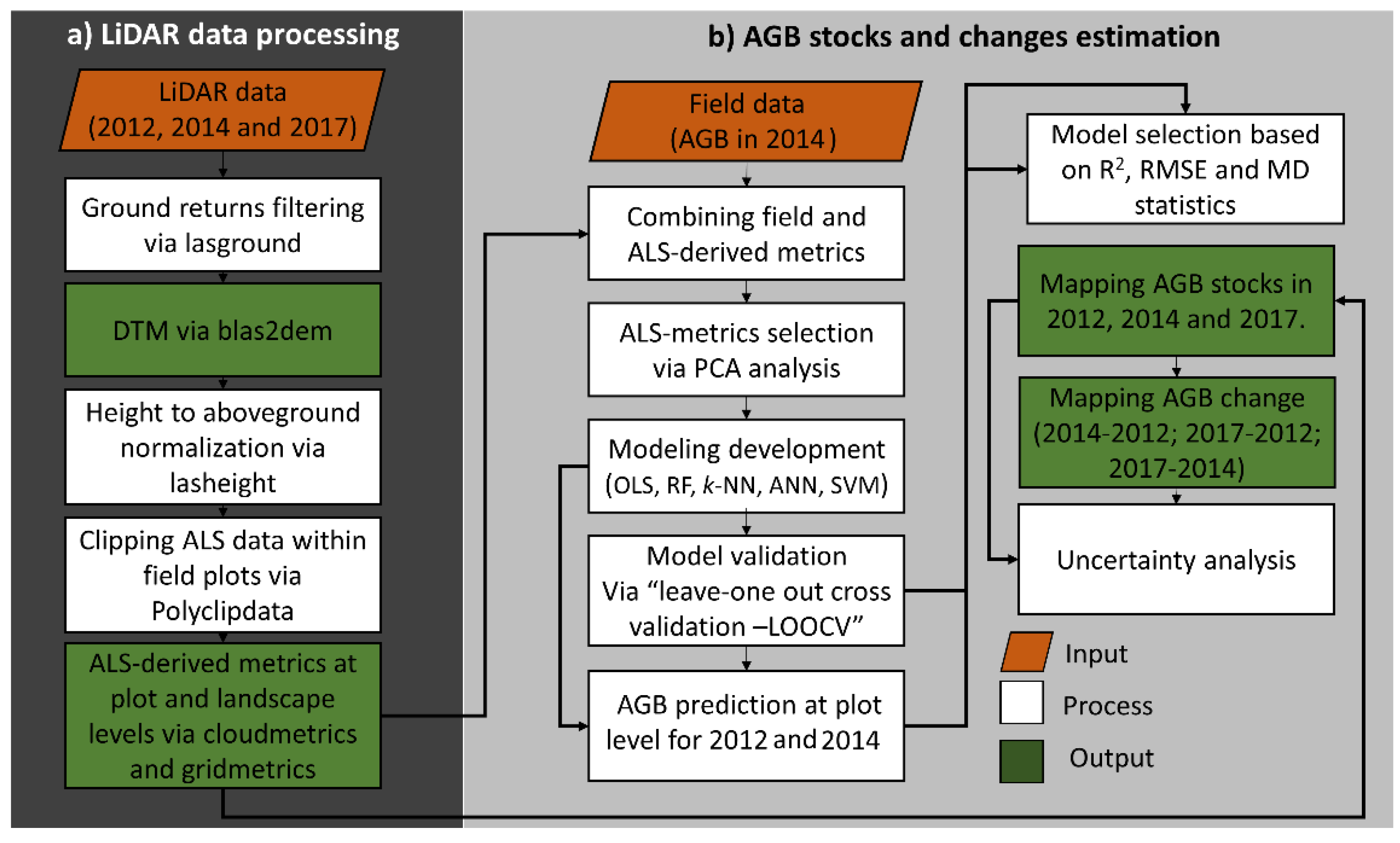
2.3. Lidar Data and Processing

LiDAR datasets were collected in 2012, 2014, and 2017 as a part of ‘Sustainable Landscapes Brazil’, a joint venture of the Brazilian Corporation of Agricultural Research (EMBRAPA) and the United States Forest Service (USFS). The attributes of the lidar sensor and flight parameters are displayed in

Table 2. Details of LiDAR data acquisitions.

Specifications	2012	2014	2017
LiDAR system	ALTM 3100	ALTM 300	ALTM 3100
Acquisition date	27–29 July	26–27 December	12 December
Datum	Sirgas 2000	Sirgas 2000	Sirgas 2000
Pulse density (pulses/m2)	13.89	37.5	22.61
Flying height (m)	850 m	850 m	850 m
Field of view (°)	11	12	15
Scanning Frequency (Hz)	59.8	83.0	40
Overlap Percentage (%)	65	65	70

.

LiDAR data processing was carried out using FUSION/LDV version 3.60 software [37] and Lastools [38]. First, LiDAR pulse density was standardized across all years to a common density of 12 pulses/m² using the algorithm implemented in the ThinData utility of the FUSION toolkit [37]. Then lasground was used to classify ground returns (step: 10 m, bulge: 0.5 m, spike: 1 m, offset: 0.05 m). From classified ground returns, DTMs (resolution: 1 m) were created via blast2dem. The calculation of heights above ground (also called normalisation) was performed by the lasheight tool, the PolyClipdata tool clipped the LiDAR data to within the plot boundaries. Lasground, Blast2dem, lasheight, and PolyClipdata are available in the LAStools software. The CloudMetrics tool was then used to derive a suite of plot-level LiDAR canopy metrics (

Table 3. LiDAR-derived canopy metrics.

Variable	Description
HMAX	Maximum height
HMEAN	Mean height
HMODE	Modal height
HSD	Height standard deviation
HVAR	Height variance
HCV	Height coefficient of variation
HIQ	Height interquartile distance
HSKE	Height skewness
HKUR	Height kurtosis
H20TH	Height 20th percentile
H25TH	Height 25th percentile
H30TH	Height 30th percentile
H40TH	Height 40th percentile
H50TH	Height 50th percentile
H60TH	Height 60th percentile
H70TH	Height 70th percentile
H75TH	Height 75th percentile
H80TH	Height 80th percentile
H90TH	Height 90th percentile
H95TH	Height 95th percentile
H99TH	Height 99th percentile
CR	Canopy relief ratio ((HMEAN − HMIN)/(HMAX − HMIN))
COV	Canopy cover (percentage of first return above 2.00 m)

); for that, we used the FUSION toolkit. A complete description of the LiDAR-derived canopy height metrics can be found in Mcgaughey [37].

2.4. Model Development and Assessment

Modelling variable selection was conducted through principal component analysis (PCA) [39] according to Silva et al. [40]. Eigenvectors were identified and inspected for each principal component, using the function “prcomp” in R [41]; a detailed description of the PCA algorithm can be found in Fernandez et al. [42]. After variable selection, we tested nine statistical model approaches for estimating and mapping AGB stock and changes as follows:

(i)

Ordinary Least Squares (OLS) regression. This is a common method for modelling and predicting AGB from LiDAR metrics. The OLS model was implemented in R with the “lm” function.

(ii)

Random Forest (RF). The RF algorithm was implemented in R using the randomForest package [43]. In RF, ntree was set to 1000, and the other parameters (e.g. mtry) were left in RF default mode.

(iii)

k-Nearest Neighbour (k-NN) imputation. This is a non-parametric method used for regression and classification [44]. In this study, we conducted k-NN using the package yaImpute in R [45]. For each imputation, we set k = 1 neighbour to preserve the variance of the data [46]. Neighbour weighting methods used were the Euclidean (k-NN-EU), Mahalanobis (k-NN-MA), Most Similar Neighbour (k-NN-MSN), Independent Component Analysis (k-NN-ICA), Random Forest (k-NN-RF), and raw (unweighted) data (k-NN-RAW).

(iv)

Support Vector Machine (SVM). This is a non-parametric statistical method. The SVM algorithm was performed using the R package e1071 via an epsilon-regression with the default epsilon value of 0.1 [47].

(v)

Artificial neural network (ANN). Here, a simulation of a biological neural network system using mathematical modelling is performed [48]. Normally, three layers of neurons make up a neural network: an input layer, a hidden layer, and an output layer. The nnt package in R was used for the ANN [49]. The hidden layer neurons parameter was set to 40, and the input and hidden nodes were set to compute the logistic function, while the output node was set to compute a linear function. Before running ANN, the dataset was standardized.

Although machine learning methods do not require that assumptions such as normality and homogeneity of variance be met, this is not true of linear regression [50,51]. Herein, we used Shapiro–Wilk [52] and Breusch–Pagan [53] tests to evaluate the normality and heteroscedasticity of the OLS model residuals.

We used LiDAR and field data from 2014 to adjust a model relating LiDAR metrics and forest AGB. Then we employed that single model across the entire time-series, estimating AGB stocks from the LiDAR acquisitions in 2012, 2014, and 2017: Equations (2)–(4). The AGB change was computed as the difference between AGB estimations from the different time points; 2012 to 2014, 2012 to 2017, and 2014 to 2017: Equations (5)–(7):

AGB₂₀₁₂ = f (LiDAR metrics 2012; AGB in 2014)

(2)

AGB₂₀₁₄ = f (LiDAR metrics 2014; AGB in 2014)

(3)

AGB₂₀₁₇ = f (LiDAR metrics 2017; AGB in 2014)

(4)

ΔAGB_{(2012–2014)} = AGB₂₀₁₄ − AGB₂₀₁₂

(5)

ΔAGB_{(2014–2017)} = AGB₂₀₁₇ − AGB₂₀₁₄

(6)

ΔAGB_{(2012–2017)} = AGB₂₀₁₇ − AGB₂₀₁₂

(7)

where AGB_t is the AGB stock for year t and ΔAGB_t1-t2 is the AGB change between years t1 and t2, both expressed in Mg/ha. Leave-one-out cross-validation (LOOCV) was employed to assess accuracy. This is done by iteratively removing a single plot i from the total number of plots n, then using the remaining plots to fit a separate model and predict a value for the removed plot (${\widehat{y}}_i$), the prediction is then compared to the observed value ($y_i$). We calculated, in Mg/ha, absolute root mean squared error (RMSE), mean difference (MD), and the coefficient of determination (R²), in order to respectively evaluate model precision, accuracy, and agreement between the predicted and observed estimates (Equations (8)–(10)).

$$\mathrm{RMSE}=\sqrt{\frac{ {{\displaystyle \sum }}_{i=1}^n {\left({\widehat{y}}_i-y_i\right)}^2}{n} }$$

(8)

$$\mathrm{MD}=\frac{1}{n}{\displaystyle \sum }_{i=1}^n\left({\widehat{y}}_i-y_i\right)$$

(9)

$$R^2=1-\frac{{{\displaystyle \sum }}_{i=1}^n {\left(y_i-{\widehat{y}}_i\right)}^2}{{{\displaystyle \sum }}_{i=1}^n\left(y_i-\overline{y}\right)}$$

(10)

Moreover, the relative RMSE and MD (in %) were calculated as a percentage of the observed mean AGB ($\overline{y}$).

The mean estimator for the AGB stocks in 2012 (${\widehat{AGB}}_{2012}$), 2014 (${\widehat{AGB}}_{2014})$ and 2017 (${\widehat{AGB}}_{2017}$) and changes at the landscape level within unlogged and logged by RIL units were calculated (Equations (11)–(13)) following McRoberts et al. [54]:

$${\widehat{AGB}}_{2012}=\frac{1}{N^2}{\displaystyle \sum }_{i=1}^{N}AG{B}_{i_{2012}}$$

(11)

$${\widehat{AGB}}_{2014}=\frac{1}{N^2}{\displaystyle \sum }_{i=1}^{N}AG{B}_{i_{2014}}$$

(12)

$${\widehat{AGB}}_{2017}=\frac{1}{N²}{\displaystyle \sum }_{i=1}^{N}AG{B}_{i_{2017}}$$

(13)

$$\widehat{{\Delta }_{AGB\left(t1-t2\right)} }=\frac{1}{N}{\displaystyle \sum }_{i=1}^N\left({\widehat{AGB}}_i^{t2}-{\widehat{AGB}}_i^{t1}\right)-\frac{1}{n}{\displaystyle \sum }_{p_i\in S}^{}\left[\left({\widehat{AGB}}_i^{t2}-{\widehat{AGB}}_i^{t1}\right)-\left(AG{B}_i^{t2}-AG{B}_i^{t1}\right)\right]$$

(14)

where N is the population size (number of pixels in the area); n is the sample size; $AG{B}_{i_{2012}}$, $AG{B}_{i_{2014}}$ and $AG{B}_{i_{2017}}$ are the estimated AGB stocks in 2012, 2014, and 2017 at the pixel i, respectively; ${\widehat{AGB}}_i^{t2}$ is the model prediction at different times, and ${\widehat{AGB}}_i^{t1}$ represents the reference biomass at each time. The second element of Equation (14) represents the bias of the initial biomass change estimator.

An uncertainty analysis of ${\widehat{AGB}}_{2012}$, ${\widehat{AGB}}_{2014}$ and ${\widehat{AGB}}_{2017}$ was conducted at the landscape level by integrating errors at the pixel level and compensating for spatial autocorrelation of errors as follows [55,56] (Equation (15)):

$$\widehat{\mathsf{\sigma }{²}_{AGB}}=\frac{1}{N²}{\displaystyle \sum }_{i=1}^N{\displaystyle \sum }_{i<j}^{N}cov\left(\sigma i,\sigma j\right)=\frac{1}{N²}\left({\displaystyle \sum }_{i=1}^N{\sigma }^2+2{\displaystyle \sum }_{i=1}^N{\displaystyle \sum }_{i<j}^N\rho \left(d\right)\sigma i\sigma j\right)$$

(15)

where $\widehat{\mathsf{\sigma }{²}_{AGB}}$ is the variance of the estimator of the mean AGB stock; ρ(d) is the spatial autocorrelation function of distance d, based on an exponential semivariogram model; and σj is the estimated standard error of AGB stock values at the j-th pixel.

The variance of the estimator for $\widehat{{\mathsf{\Delta }}_{AGB\left(t1-t2\right)}}$ was computed as (Equation (16)):

$$\widehat{Var}\left( \widehat{{\mathsf{\Delta }}_{AGB\left(t1-t2\right)}}\right)=\frac{1}{n\left(n-1\right)}{\displaystyle \sum }_{p_i\in S}^{ }\left[{\epsilon }_i-\overline{\epsilon }\right]$$

(16)

where ${\epsilon }_i$ is model prediction error and $\overline{\epsilon }$ is mean model error.

3. Results

3.1. Principal Component Analysis (PCA) and Variable Selection

The PCA indicated that 97% of the variance in the suite of LiDAR metrics is accounted for by the first six principal components (Figure 3). For each of these principal components, one metric was selected on the basis of the highest contained value of eigenvectors. The selected metrics were: PC1: Mean height (HMEAN); PC2: Height coefficient of variation (HCV); PC3: Height kurtosis (HKUR); PC4: Canopy cover (COV); PC5: Modal height (HMODE); PC6: Height skewness (HSKEW). Therefore, we selected only these metrics for modelling AGB, thus reducing dataset size and redundancy. The contribution of each PC to the total variance and the projection of each metric are shown in Figure 3.

Table 4. Eigenvalues and eigenvectors for the first six principal components and selected LiDAR metrics.

PCs	Ev	Eigenvectors (Eg)
		HMEAN	HCV	HKUR	COV	HMODE	HSKEW
PC1	3.27	−0.30	0.11	−0.05	0.02	−0.17	0.13
PC2	2.50	−0.04	0.36	−0.17	−0.10	−0.17	0.27
PC3	1.67	0.05	−0.09	0.45	0.33	0.02	0.31
PC4	0.89	0.03	−0.05	−0.38	0.85	0.14	0.09
PC5	0.77	0.09	−0.10	0.05	0.05	−0.88	0.07
PC6	0.60	−0.05	0.12	0.29	0.35	−0.30	−0.38

represents the eigenvalues and eigenvectors of each principal component.

PC is the given Principal Component; Ev is the Eigenvalues for each PC. Bold values indicate the largest contributing LiDAR metric for a given PC.

3.2. Model Performance

The best modelling approach for estimating AGB according to the LOOCV procedure was the OLS, which produced a relative RMSE less than 20% (

Table 5. Aboveground biomass (AGB) model precision and accuracy derived from the LOOCV procedure. Average and standard deviation of predicted AGB (Mg/ha) stocks at plot level in 2014.

Method	R2	RMSE		MD		LiDAR-Derived AGB (Mg/ha) Stock in 2014
		Mg/ha	%	Mg/ha	%
OLS	0.70	46.94	19.71	−0.57	−0.24	237.54 ± 74.56
RF	0.59	55.44	23.29	−0.16	−0.07	237.94 ± 57.77
k–NN-RAW	0.35	75.90	31.87	−1.54	−0.65	236.56 ± 81.97
k-NN-EU	0.48	66.90	28.09	−4.09	−1.72	234.01 ± 84.29
k–NN-MA	0.39	73.01	30.66	−4.66	−1.96	233.44 ± 81.64
k-NN-MSN	0.53	64.61	27.09	−4.39	−1.94	233.71 ± 89.04
k-NN-ICA	0.38	73.01	30.66	−4.66	−1.96	233.44 ± 81.64
k-NN-RF	0.40	74.71	31.21	−3.43	−1.44	234.67 ± 88.50
SVM	0.57	56.24	23.62	1.59	0.67	239.69 ± 60.93
ANN	0.61	54.48	22.89	0.09	0.03	238.20 ± 76.72

). Shapiro–Wilk, and Breusch–Pagan showed that the assumptions of the linear regression were not violated (p-value > 0.05).

RF, SVM, and ANN showed slightly lower MD than OLS; however, the accuracy was inferior in terms of R² and RMSE. The k-NN algorithm had six derivations tested, with R² values varying from 0.35 to 0.53. Relative RMSE values ranged from 27.10% to 31.87%, while relative MD values varied from –1.96 to –0.65%, respectively. Among the k-NN variants, the k-NN-MSN model had the best performance, with the greatest values of R² and the lowest value of RMSE and MD. The worst performance was found for k-NN-RAW, which presented the lowest values for R² and the greatest value of RMSE and MD (Table 5).

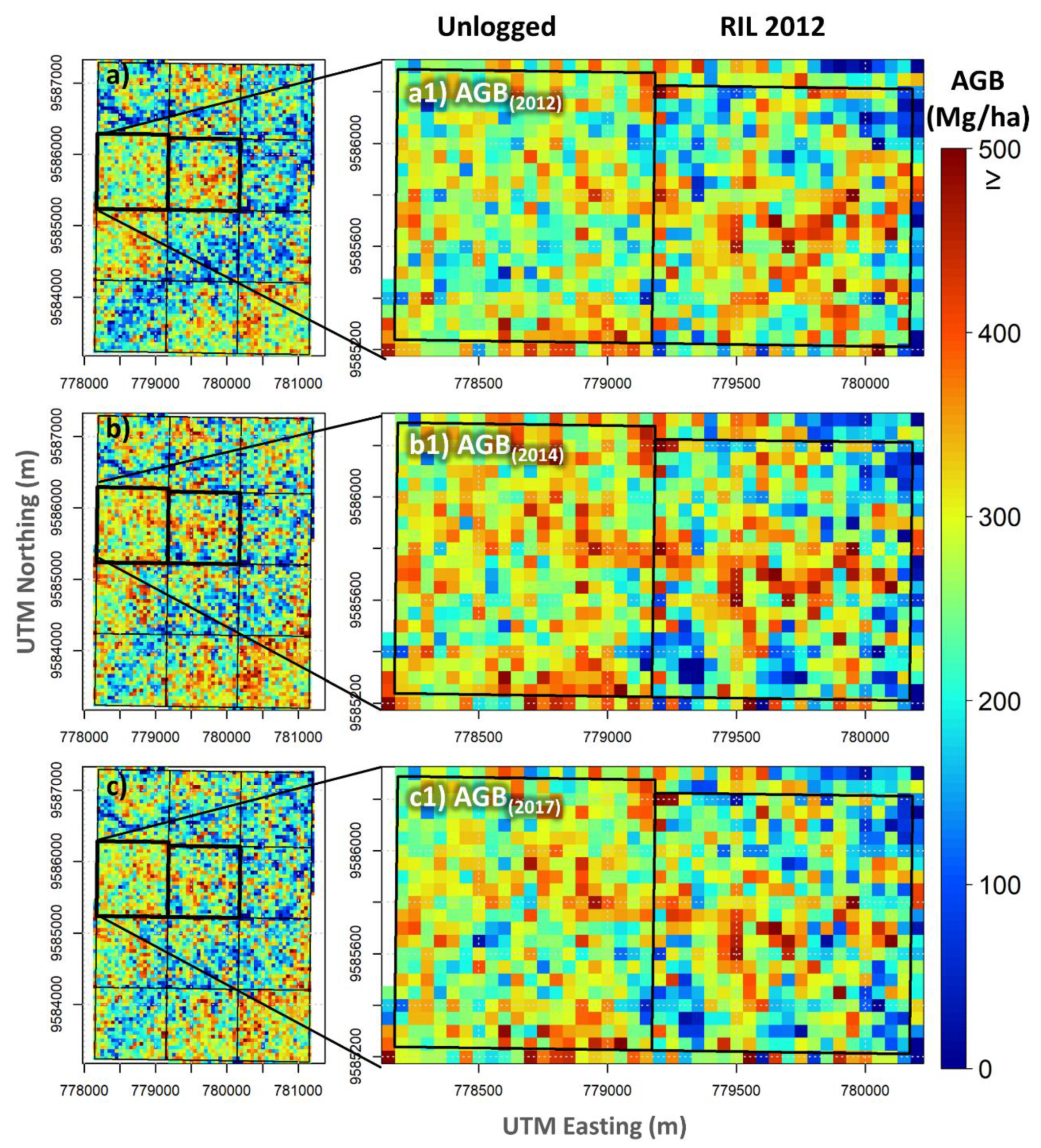
3.3. Aboveground Biomass Change Mapping and Uncertainty

Estimation of AGB stocks and AGB change at the landscape level was performed using the OLS model (

Table 6. Aboveground biomass stocks and changes estimates at landscape level derived from the OLS model for the unlogged and reduced impact logging (RIL) work units (UT) within each year of logging. Std Error is the estimated standard error of the estimator for the mean aboveground biomass (AGB) stock and AGB changes derived from the uncertainty analysis.

Work Unit (UT)		$\mathbf{A}\mathbf{G}{\mathbf{B}}_{2012}(\mathbf{Mg}/\mathbf{ha})$			$\mathbf{A}\mathbf{G}{\mathbf{B}}_{2014}(\mathbf{Mg}/\mathbf{ha})$			$\mathbf{A}\mathbf{G}{\mathbf{B}}_{2017}(\mathbf{Mg}/\mathbf{ha})$			$\mathbf{∆}\mathbf{A}\mathbf{G}{\mathbf{B}}_{\left(2012–2014\right)}(\mathbf{Mg}/\mathbf{ha})$			$\mathbf{∆}\mathbf{A}\mathbf{G}{\mathbf{B}}_{\left(2014–2017\right)}(\mathbf{Mg}/\mathbf{ha})$			$\mathbf{∆}\mathbf{A}\mathbf{G}{\mathbf{B}}_{\left(2012–2017\right)}(\mathbf{Mg}/\mathbf{ha})$
		Mean	sd	std Error	Mean	sd	std Error	Mean	sd	std Error	Mean	sd	std Error	Mean	sd	std Error	Mean	sd	std Error
RIL	2006	112.85	683.75	4.94	220.69	104.75	5.04	193.11	252.29	5.07	107.84	665.07	2.38	−27.58	225.25	1.88	80.26	703.70	2.90
	2007	224.11	95.58	4.28	263.18	93.90	4.37	232.94	171.30	4.38	39.07	38.03	2.70	−30.24	146.12	2.43	8.83	148.94	2.97
	2008	198.68	109.30	4.94	234.89	108.52	5.16	230.90	103.03	4.90	36.21	39.63	1.92	−3.99	40.88	2.01	32.22	55.41	2.68
	2010	202.97	101.22	4.61	244.05	93.87	4.53	218.99	314.21	4.40	41.08	36.17	1.71	−25.07	299.06	1.92	16.02	300.80	2.59
	2012	264.54	239.32	4.60	252.27	111.26	5.24	242.47	100.24	4.75	−12.27	229.46	3.73	−9.80	55.19	2.60	−22.07	228.75	3.85
	2013	289.88	82.47	3.92	275.22	95.75	4.75	259.74	92.83	4.58	−14.66	71.37	3.53	−15.47	38.58	1.90	−30.14	69.93	3.48
Unlogged		284.58	71.48	3.44	312.09	74.58	3.59	294.29	74.25	3.60	27.51	32.16	2.68	−17.80	38.08	1.86	9.71	46.76	2.29

). Figure 4 shows AGB stocks, while Figure 5 reports the AGB change derived from AGB stock maps and highlights these estimations at both unlogged and logged areas. The AGB estimates generated by the best model (OLS) allowed us to observe that there were increases in AGB stocks at the landscape level. In 2012, the mean stock was 229.10 Mg/ha (sd ± 232.12), while in 2014 and 2017, it was 258.18 (sd ± 106.53) and 240.34 (sd ± 177) Mg/ha, respectively. We also observed the same pattern for the unlogged area (Figure 4a1,b1,c1), where there were increases in the order of 10 Mg/ha between the period of 2012 to 2017. However, we noticed that more recent logging areas (2010 and 2012) showed losses in the biomass stocks, while those that suffered older logging managed to recover the biomass stocks and show increases in the stocks, highlighting the area that was explored in 2006, with an increase of 80 Mg/ha, that is, an increase in the order of 13 Mg/ha per year over the evaluated period (2012 to 2017).

The mean of the AGB change at the landscape level shows changes ranging from –30.35 (sd ± 69.41) to 39.41 (sd ± 34.44) across unlogged and logged areas for the intervals of 2012–2014, 2014–2017, and 2012–2017 (Table 6 and Figure 5a–c). As expected, logged areas showed greater changes than unlogged areas. The highest AGB change of 39.41 (sd ± 34.44) Mg/ha was found in the interval from 2012 to 2014 in an area logged in 2006. The uncertainty of the estimated AGB stocks was ≤50.7 Mg/ha for 2012, 2014, and 2017 and across unlogged and logged areas, while the uncertainty of the estimated AGB change was ≤3.85 Mg/ha for 2012, 2014, and 2017 across unlogged and logged areas. The uncertainty of the estimated AGB change was ≤3.85 Mg/ha for 2012, 2014, and 2017 across unlogged and logged areas.

4. Discussion

Tracking change in AGB is vital for monitoring, reporting, and verification protocols (MRV) in support of REDD+. For accurate and satisfactory estimations, proper modelling techniques and data acquisition procedures are necessary. In our study, we developed maps of AGB stocks using multi-temporal LiDAR data and advanced modelling techniques that show the variation of AGB stocks over the years for logged forests in eastern Amazonia. Owing to the subtle and short-term changes occurring, logged forests are one of the hardest in which to detect changes. Results from our study highlight the robustness of our framework, the potential of multi-temporal LiDAR, and the importance of appropriate modelling techniques in support of climate change mitigation initiatives. By comparing AGB change between logged and intact forests, we gained insight into tropical forest resilience to disturbance. Specifically, our findings indicate that tropical forests have great potential for AGB recovery even after disturbances such as selective logging.

To predict biophysically important forest attributes such as basal area, mean stem diameter, and AGB, LiDAR measurements derived from point clouds can be used in empirical models [57,58,59,60]. In our study, the metrics selected to compose the models are corroborated by previous studies [59,61]. For instance, numerous AGB estimation studies [62,63,64] had indicated the metric ‘mean canopy height’ to be one of the most significant attributes, and this is reflected by our PCA results. Likewise, metrics such as Standard Deviation and Coefficient of Variation of Height were found to provide information on the vertical complexity and heterogeneity of canopy components [65]. In addition, our results support the findings of some previous studies that assessed the capacity of LiDAR data point-based metrics to describe forest biophysical parameters, using results obtained from point density [61] and the Canopy Cover metric [66,67]. Nonetheless, it might be possible to estimate AGB with the help of several other ALS-derived metrics [68,69] as well as with more simplified model structures, while being able to attain similar levels of accuracy as reported in our study. This would be an interesting area to explore in the near future.

In studies aimed to estimate AGB stock and AGB change, the selection of the appropriate modelling approach is one of the most critical steps [59]. We found, through the use of LOOCV, that OLS performed better than non-parametric approaches; a finding which has been reported in other studies comparing modelling methods in predicting various forest attributes [70,71,72]. By comparing the performance of OLS with other methods, we further evaluated how much variation is happening with AGB estimation varies and what trade-offs may be associated with different methods while working with logged forests. Additionally, we demonstrate that methods such as RF and SVM that performed close to the OLS can be used to estimate and make inferences when necessary; that is, in situations where there exist non-linear or diverse relationships between dependent and independent variables [73]. The performances of RF and SVM, as the best among non-parametric approaches, may have been affected not only by the number of field plots but also by other factors such as bootstrapping of data to avoid overfitting R² values [74].

In the case of k-NN based methods, we noticed comparatively less satisfactory results, even after feature scaling. Hudak et al. [46] compared different k-NN imputations to simultaneously impute the basal area and plot density per species from topographic variables and LiDAR-derived canopy structure. They concluded that k-NN was inferior to RF, reflecting our results. This can be tied to the fact that this algorithm uses the training data for classification rather than for learning and improving the model, and is very sensitive to noisy data, missing values, outliers, and dimensionality; additional difficulty rests in determining the value of parameter K on a case-by-case basis. We also found the computational cost to be quite high here as we had to calculate the distance of each instance under consideration to all the training samples. In general, apart from the dilemma with attribute selection—which might have contributed to the poor performance in our case—we had selected the same metrics for all the models built; another critical issue while employing k-NN is the uncertainty in choosing the appropriate kind of distance-based learning. In our study, we did include six different types of distances and were able to compare their performances. Given the low performances and minimal variations, in terms of RMSE and MD, between different distance-based learning methods, further research is encouraged before considering k-NN based techniques for similar studies. As previous studies have recommended, k-NN-based approaches can be more reliable when a design-based framework of forest inventory with non-parametric based estimators is involved, because this method accounts for dependence and heteroscedasticity in the data [73,75].

Asner et al. [76] compared the accuracies of non-parametric AGB models integrating LiDAR and optical data in a forest in northwestern China and found that among non-parametric approaches, RF performed best, followed by Back Propagation Neural Networks and SVR. The results of Asner et al. [76] show improvements in AGB estimates by integrating LiDAR and optical data and present a pattern similar to that of this study. Görgens et al. [77] conducted a study with very similar results to our own, in which the authors found superior RF performance as compared with other machine learning approaches such as ANN and SVR. On the other hand, there have been studies conducted based on non-linear regression models as well. For instance, Shao et al. [26], for estimating AGB, employed a multiplicative non-linear regression model that took into consideration both lidar-derived metrics as well soil-based site productivity class data. Herein, the authors were able to address a few critical issues associated with mixed forests, such as the overlooked differences in height-diameter relationships with respect to sites and species found within, resulting from varied site productivities and the similarity of the vertical height profiles with varied tree volume/density arising from the deliquescent growth form of hardwood trees; not to mention, these concerns are ubiquitous and extremely challenging in the realm of tropical forests. The authors reported the relationship between AGB and LiDAR-based metrics to be nonlinear in case of low productivity sites and predominantly linear on high productivity sites.

When making comparisons to other studies, we concluded that the results of our research, in terms of R² for AGB estimates, fall within the bounds of that which has been found in tropical forest areas [18,76]. Asner et al. [76] in four tropical regions located in Madagascar, Peru, Panama, and Hawaii, reported R² varying between 0.68 to 0.85. A study in selectively logged tropical forest by d’Oliveira et al. [78] found values of R² ranging from 0.63–0.72 for linear regression models, as the authors expected, owing to their restriction to a single allometric AGB equation exclusively based upon the diameter for all species, akin to our study. Englhart et al. [16] emphasized multi-temporal LiDAR’s power in accurately quantifying tree height change and associated AGB, necessary for REDD+, even for very small areas/plots.

Regarding the mean AGB densities in Mg/ha, the values we found agree with findings from other studies conducted in tropical forests. Authors such as d’Oliveira et al. [78] used airborne LiDAR data to estimate AGB and to identify regions impacted by selective logging across tropical forests in the western Brazilian Amazon, and the mean AGB they found was of 231.6 Mg/ha. Andersen et al. [25] estimated the AGB for two years, 2010 and 2011, and obtained the mean values of 232.1 and 223.0 Mg/ha, respectively, and AGB change of −9.1 Mg/ha for the period evaluated. The mean change in AGB stocks observed in Andersen et al. [25] is similar to the values found in this study. It should be noted that the higher estimated values in this study are justified owing to the analysis intervals also being larger. Furthermore, in our results, we noticed the largest decrease (−30.24 Mg/ha) in AGB stocks between 2014 and 2017 in a logged area (−10.0 Mg/ha per year); however, when analyzing the entire period (2012 to 2017), it shows a gain of approximately 8 Mg/ha. In other words, over the entire evaluated period, it was possible to verify the increase in biomass stocks and not the decrease as seen first, perhaps reflecting the balance between increased growth and increased mortality in the explored locations [35]. For this reason, we believe that studies in this scope need longer assessment times as they may otherwise result in hasty conclusions. Rangel Pinagé et al. [35] cited a series of studies on mortality after logging and also commented on the need for investigations with larger time spans and different logging intensities to determine the persistence of logging impacts on the canopy. In addition, we estimated slightly higher gains in forests logged before the first LiDAR acquisition (2012) than in intact forests (mean biomass gains of 20.0 Mg/ha in logged areas and for unlogged forests mean biomass gains of 7.0 Mg/ha, both for the period 2012–2014). Moreover, the logged areas and the unlogged areas do not differ widely in terms of values and appear to be gaining biomass at similar rates.

Based on our results, there are four areas where future studies could focus: scaling approaches, quantifying impacts of other phases of logging on AGB, and exploring other concomitant factors that affect carbon release, and the influence of site productivity variations and multiple tree species presence on AGB change. For instance, scaling up could be done through the use of full-waveform LiDAR, which can cover larger areas. Recent studies have shown that the results from discrete return and full-waveform LiDAR are of comparable accuracy [79]. Since LiDAR surveys are expensive, another option is to scale up regional estimations of AGB and AGB change with satellite imagery [16,80]. Through merging data sources, it is possible to perform a classification approach versus regression approach as well—for example, by making use of modelling techniques such as random forest—for identifying and isolating logged areas and then for comparing their AGB estimation capabilities. It should be noted that the primary changes in AGB in this study were caused by felling trees; however, future studies should also focus on quantifying the impacts on AGB caused by other phases of selective logging; such as the construction of roads and log landings. Additionally, it could be intriguing to explore how other concomitant factors such as increased forest fires due to logging, damages from machinery related to logging, and forest degradation affect carbon. Lastly, we recommend more research to investigate the influence of different tree species being present and forest types in AGB change, as previous studies [16] have reported that logged forests experience higher growth rates and accumulate more AGB than unaffected primary forests. On a similar theme, if we could stretch the data collection paradigms whenever possible to include direct or indirect measures of site productivity details, that would allow us to substantially improve the predictive capability of AGB models, as issues associated with lidar-height-based metrics can be kept minimal as discussed in Shao et al. [26].

5. Conclusions

In our study, we modelled AGB in a selectively logged Amazonian tropical forest using field data and LiDAR-derived metrics. In addition, we tested different approaches based on non-parametric methods to estimate AGB at the plot level and compared it with parametric OLS. Our comparison of the methods for estimations has shown that OLS is the most suitable method for AGB estimation using airborne LiDAR, as indicated by R², RMSE, and MD. We also demonstrated that other methods like RF, SVM, and ANN have the potential for predicting AGB when a non-parametric method is required. Our results show that OLS can be used to estimate AGB with satisfactory accuracy and that repeated LiDAR measurements over time are capable of estimating AGB change at landscape levels. While field data for 2012 and 2017 would have allowed us to evaluate if the same parameters and models work best for all the cases, these results remain robust. LiDAR-based approaches allow us to address questions of changing ABG with increasing speed, scale, and reliability. Our study effectively demonstrated this capacity by finding that LiDAR has the capability of tracking even the small-scale differences happening within logged forests with satisfiable accuracies.

References

1. Gibbs, H.K.; Brown, S.; Niles, J.O.; Foley, J.A. Monitoring and estimating tropical forest carbon stocks: Making REDD a reality. Environ. Res. Lett. 2007, 2, 045023. [Google Scholar] [CrossRef]
2. Thomson, A.M.; Calvin, K.V.; Chini, L.P.; Hurtt, G.; Edmonds, J.A.; Bond-Lamberty, B.; Janetos, A.C. Climate mitigation and the future of tropical landscapes. Proc. Natl. Acad. Sci. USA 2010, 107, 19633–19638. [Google Scholar] [CrossRef] [PubMed] [Green Version]
3. Phillips, O.L.; Lewis, S.L.; Baker, T.R.; Chao, K.J.; Higuchi, N. The changing Amazon forest. Philos. Trans. R. Soc. B 2008, 363, 1819–1827. [Google Scholar] [CrossRef] [PubMed] [Green Version]
4. Malhi, Y.; Roberts, J.T.; Betts, R.A.; Killeen, T.J.; Li, W.; Nobre, C.A. Climate change, deforestation, and the fate of the Amazon. Science 2008, 319, 169–172. [Google Scholar] [CrossRef] [Green Version]
5. Silva, C.A.; Valbuena, R.; Pinagé, E.R.; Mohan, M.; de Almeida, D.R.; North Broadbent, E.; Klauberg, C. ForestGapR: An r Package for forest gap analysis from canopy height models. Methods Ecol. Evol. 2019, 10, 1347–1356. [Google Scholar] [CrossRef] [Green Version]
6. Chazdon, R.L. Tropical forest recovery: Legacies of human impact and natural disturbances. Perspect Plant. Ecol. 2003, 6, 51–71. [Google Scholar] [CrossRef] [Green Version]
7. Miles, L.; Kapos, V. Reducing greenhouse gas emissions from deforestation and forest degradation: Global land-use implications. Science 2008, 320, 1454–1455. [Google Scholar] [CrossRef] [Green Version]
8. Marvin, D.C.; Asner, G.P.; Knapp, D.E.; Anderson, C.B.; Martin, R.E.; Sinca, F.; Tupayachi, R. Amazonian landscapes and the bias in field studies of forest structure and biomass. Proc. Natl. Acad. Sci. USA 2014, 111, 5224–5232. [Google Scholar] [CrossRef] [Green Version]
9. Molina, P.; Asner, G.; Farjas Abadía, M.; Ojeda Manrique, J.; Sánchez Diez, L.; Valencia, R. Spatially-explicit testing of a general aboveground carbon density estimation model in a western Amazonian forest using airborne LiDAR. Remote Sens. 2016, 8, 9. [Google Scholar] [CrossRef] [Green Version]
10. Laurin, G.V.; Chan, J.C.W.; Chen, Q.; Lindsell, J.A.; Coomes, D.A.; Guerriero, L.; Valentini, R. Biodiversity mapping in a tropical West African forest with airborne hyperspectral data. PLoS ONE 2014, 9, 97910. [Google Scholar] [CrossRef]
11. Asner, G.P.; Knapp, D.E.; Broadbent, E.N.; Oliveira, P.J.; Keller, M.; Silva, J.N. Selective logging in the Brazilian Amazon. Science 2005, 310, 480–482. [Google Scholar] [CrossRef] [PubMed]
12. Pearson, T.R.; Brown, S.; Casarim, F.M. Carbon emissions from tropical forest degradation caused by logging. Environ. Res. Lett. 2014, 9, 034017. [Google Scholar] [CrossRef] [Green Version]
13. Mazzei, L.; Sist, P.; Ruschel, A.; Putz, F.E.; Marco, P.; Pena, W.; Ferreira, J.E.R. Above-ground biomass dynamics after reduced-impact logging in the Eastern Amazon. For. Ecol. Manag. 2010, 259, 367–373. [Google Scholar] [CrossRef]
14. Rutishauser, E.; Hérault, B.; Baraloto, C.; Blanc, L.; Descroix, L.; Sotta, E.D.; De Oliveira, L.C. Rapid tree carbon stock recovery in managed Amazonian forests. Curr. Biol. 2015, 25, 787–788. [Google Scholar] [CrossRef] [Green Version]
15. Silva, C.; Hudak, A.; Vierling, L.; Klauberg, C.; Garcia, M.; Ferraz, A.; Saatchi, S. Impacts of airborne lidar pulse density on estimating biomass stocks and changes in a selectively logged tropical forest. Remote Sens. 2017, 9, 1068. [Google Scholar] [CrossRef] [Green Version]
16. Englhart, S.; Jubanski, J.; Siegert, F. Quantifying dynamics in tropical peat swamp forest biomass with multi-temporal LiDAR datasets. Remote Sens. 2013, 5, 2368–2388. [Google Scholar] [CrossRef] [Green Version]
17. Zolkos, S.G.; Goetz, S.J.; Dubayah, R. A meta-analysis of terrestrial aboveground biomass estimation using lidar remote sensing. Remote Sens. Environ. 2013, 128, 289–298. [Google Scholar] [CrossRef]
18. Asner, G.P.; Hughes, R.F.; Varga, T.A.; Knapp, D.E.; Kennedy-Bowdoin, T. Environmental and biotic controls over aboveground biomass throughout a tropical rain forest. Ecosystems 2009, 12, 261–278. [Google Scholar] [CrossRef]
19. Clark, M.L.; Roberts, D.A.; Ewel, J.J.; Clark, D.B. Estimation of tropical rain forest aboveground biomass with small-footprint lidar and hyperspectral sensors. Remote Sens. Environ. 2011, 115, 2931–2942. [Google Scholar] [CrossRef]
20. Houghton, R.A. Aboveground forest biomass and the global carbon balance. Glob. Chang. Biol. 2005, 11, 945–958. [Google Scholar] [CrossRef]
21. Lei, Y.; Treuhaft, R.; Keller, M.; dos-Santos, M.; Gonçalves, F.; Neumann, M. Quantification of selective logging in tropical forest with spaceborne SAR interferometry. Remote Sens. Environ. 2018, 211, 167–183. [Google Scholar] [CrossRef]
22. Hethcoat, M.G.; Edwards, D.P.; Carreiras, J.M.; Bryant, R.G.; Franca, F.M.; Quegan, S. A machine learning approach to map tropical selective logging. Remote Sens. Environ. 2019, 221, 569–582. [Google Scholar] [CrossRef]
23. Koch, B. Status and future of laser scanning, synthetic aperture radar and hyperspectral remote sensing data for forest biomass assessment. ISPRS J. Photogramm. Remote Sens. 2010, 65, 581–590. [Google Scholar] [CrossRef]
24. Gleason, C.J.; Im, J. Forest biomass estimation from airborne LiDAR data using machine learning approaches. Remote Sens. Environ. 2012, 125, 80–91. [Google Scholar] [CrossRef]
25. Andersen, H.E.; Reutebuch, S.E.; McGaughey, R.J.; d’Oliveira, M.V.; Keller, M. Monitoring selective logging in western Amazonia with repeat lidar flights. Remote Sens. Environ. 2014, 151, 157–165. [Google Scholar] [CrossRef] [Green Version]
26. Shao, G.; Shao, G.; Gallion, J.; Saunders, M.R.; Frankenberger, J.R.; Fei, S. Improving Lidar-based aboveground biomass estimation of temperate hardwood forests with varying site productivity. Remote Sens. Environ. 2018, 204, 872–882. [Google Scholar] [CrossRef]
27. Domingo, D.; Lamelas, M.T.; Montealegre, A.L.; García-Martín, A.; de la Riva, J. Estimation of Total Biomass in Aleppo Pine Forest Stands Applying Parametric and Nonparametric Methods to Low-Density Airborne Laser Scanning Data. Forests 2018, 9, 158–175. [Google Scholar] [CrossRef] [Green Version]
28. Domingo, D.; Lamelas, M.T.; Montealegre, A.L.; de la Riva, J. Comparison of regression models to estimate biomass losses and CO emissions using low density airborne laser scanning data in a burnt Aleppo pine forest. Eur. J. Remote Sens. 2017, 50, 384–396. [Google Scholar] [CrossRef] [Green Version]
29. Latifi, H.; Nothdurft, A.; Koch, B. Non-parametric prediction and mapping of standing timber volume and biomass in a temperate forest: Application of multiple optical/LiDAR-derived predictors. Forestry 2010, 83, 395–407. [Google Scholar] [CrossRef] [Green Version]
30. Gagliasso, D.; Hummel, S.; Temesgen, H. A comparison of selected parametric and non-parametric imputation methods for estimating forest biomass and basal area. Open J. For. 2014, 4, 42–48. [Google Scholar] [CrossRef] [Green Version]
31. Costa, M.H.; Foley, J.A. A comparison of precipitation datasets for the Amazon basin. Geophys. Res. Lett. 1998, 25, 155–158. [Google Scholar] [CrossRef]
32. Holmes, T.P.; Blate, G.M.; Zweede, J.C.; Pereira, R., Jr.; Barreto, P.; Boltz, F.; Bauch, R. Financial and ecological indicators of reduced impact logging performance in the eastern Amazon. For. Ecol. Manag. 2002, 163, 93–110. [Google Scholar] [CrossRef]
33. Radambrasil, P. Projeto Radambrasil: 1973–1983, Levantamento de Recursos Naturais. Energia; Ministério das Minas e Energia, Departamento Nacional de Produção Mineral (DNPM): Rio de Janeiro, Brazil, 1983; Volumes 1–23. [Google Scholar]
34. Pereira, R., Jr.; Zweede, J.; Asner, G.P.; Keller, M. Forest canopy damage and recovery in reduced-impact and conventional selective logging in eastern Para, Brazil. For. Ecol. Manag. 2002, 168, 77–89. [Google Scholar] [CrossRef]
35. Rangel Pinagé, E.; Keller, M.; Duffy, P.; Longo, M.; Dos-Santos, M.N.; Morton, D.C. Long-term impacts of selective logging on Amazon Forest dynamics from multi-temporal airborne LiDAR. Remote Sens. 2019, 11, 709. [Google Scholar] [CrossRef] [Green Version]
36. Chave, J.; Réjou-Méchain, M.; Búrquez, A.; Chidumayo, E.; Colgan, M.S.; Delitti, W.B.; Henry, M. Improved allometric models to estimate the aboveground biomass of tropical trees. Glob. Chang. Biol. 2014, 20, 3177–3190. [Google Scholar] [CrossRef]
37. Mcgaughey, R.J.M.; FUSION/LDV: Software for LiDAR Data Analysis and Visualization (Version 3.80). Seattle, WA. Available online: http://forsys.cfr.washington.edu/fusion/fusionlatest.html (accessed on 15 October 2019).
38. Isenburg, M. LAStools—Efficient Tools for Lidar Processing. Available online: http://www.cs.unc.edu/~isenburg/lastools/ (accessed on 8 March 2018).
39. Wold, S.; Esbensen, K.; Geladi, P. Principal component analysis. Chemom. Intell. Lab. 1987, 2, 37–52. [Google Scholar] [CrossRef]
40. Silva, C.A.; Klauberg, C.; Hudak, A.T.; Vierling, L.A.; Liesenberg, V.; Carvalho, S.P.E.; Rodriguez, L.C. A principal component approach for predicting the stem volume in Eucalyptus plantations in Brazil using airborne LiDAR data. For. Int. J. For. Res. 2016, 89, 422–433. [Google Scholar] [CrossRef]
41. R Core Team. R: A Language and Environment for Statistical Computing; Version 3.6.1; R Foundation for Statistical Computing: Vienna, Austria, 2019. [Google Scholar]
42. Fernandez, D.; Gonzalez, C.; Mozos, D.; Lopez, S. FPGA implementation of the principal component analysis algorithm for dimensionality reduction of hyperspectral images. J. Real Time Image Process. 2019, 16, 1395–1406. [Google Scholar] [CrossRef]
43. Liaw, A.; Wiener, M. Classification and regression by randomForest. R News 2002, 2, 18–22. [Google Scholar]
44. Altman, N.S. An introduction to kernel and nearest-neighbor nonparametric regression. Am. Stat. 1992, 46, 175–185. [Google Scholar] [CrossRef] [Green Version]
45. Crookston, N.L.; Finley, A.O. YaImpute: An R package for kNN imputation. J. Stat. Softw. 2008, 23, 16. [Google Scholar] [CrossRef] [Green Version]
46. Hudak, A.T.; Crookston, N.L.; Evans, J.S.; Hall, D.E.; Falkowski, M.J. Nearest neighbor imputation of species-level, plot-scale forest structure attributes from LiDAR data. Remote Sens. Environ. 2008, 112, 2232–2245. [Google Scholar] [CrossRef] [Green Version]
47. Meyer, D.; Hornik, K.; Weingessel, A.; Chang, C.; Lin, C. Package e1071. Available online: https://cran.r-project.org/web/packages/e1071/e1071.pdf (accessed on 24 May 2019).
48. Kohonen, T. An introduction to neural computing. Neural Netw. 1988, 1, 3–16. [Google Scholar] [CrossRef]
49. Venable, W.N.; Ripley, B.D. Modern Applied Statistics with S; Springer: New York, NY, USA, 2002. [Google Scholar]
50. Manly, B.F.; Alberto, J.A.N. Multivariate Statistical Methods: A Primer, 3rd ed.; Chapman and Hall/CRC: London, UK, 2005. [Google Scholar]
51. Marcoulides, G.A.; Hershberger, S.L. Multivariate Statistical Methods: A First Course; Psychology Press: Mahwah, NJ, USA, 1997. [Google Scholar]
52. Shapiro, S.S.; Wilk, M.B. An analysis of variance test for normality (complete samples). Biometrika 1965, 52, 591–611. [Google Scholar] [CrossRef]
53. Breusch, T.S.; Pagan, A.R. A simple test for heteroscedasticity and random coefficient variation. Econom. J. Econom. Soc. 1979, 1287–1294. [Google Scholar] [CrossRef]
54. McRoberts, R.E.; Bollandsås, O.M.; Næsset, E. Modeling and Estimating Change. In Forestry Applications of Airborne Laser Scanning, Managing Forest Ecosystems; Maltamo, M., Næsset, E., Vauhkonen, J., Eds.; Springer: Berlin/Heidelberg, Germany, 2014; Volume 27. [Google Scholar]
55. McRoberts, R.E. A model-based approach to estimating forest area. Remote Sens. Environ. 2006, 103, 56–66. [Google Scholar] [CrossRef]
56. Weisbin, C.R.; Lincoln, W.; Saatchi, S. A systems engineering approach to estimating uncertainty in above-ground biomass (AGB) derived from remote-sensing data. Syst. Eng. 2014, 17, 361–373. [Google Scholar] [CrossRef]
57. Dalla Corte, A.P.; Rex, F.E.; Almeida, D.R.A.D.; Sanquetta, C.R.; Silva, C.A.; Moura, M.M.; Moraes, A.D. Measuring Individual Tree Diameter and Height Using GatorEye High-Density UAV-Lidar in an Integrated Crop-Livestock-Forest System. Remote Sens. 2020, 12, 863. [Google Scholar] [CrossRef] [Green Version]
58. Mohan, M.; de Mendonça, B.A.F.; Silva, C.A.; Klauberg, C.; de Saboya Ribeiro, A.S.; de Araújo, E.J.G.; Cardil, A. Optimizing individual tree detection accuracy and measuring forest uniformity in coconut (Cocos nucifera L.) plantations using airborne laser scanning. Ecol Model. 2019, 409, 108736. [Google Scholar] [CrossRef]
59. Fassnacht, F.E.; Hartig, F.; Latifi, H.; Berger, C.; Hernández, J.; Corvalán, P.; Koch, B. Importance of sample size, data type and prediction method for remote sensing-based estimations of aboveground forest biomass. Remote Sens. Environ. 2014, 154, 102–114. [Google Scholar] [CrossRef]
60. Rex, F.E.; Corte, A.P.D.; Machado, S.D.A.; Silva, C.A.; Sanquetta, C.R. Estimating Above-Ground Biomass of Araucaria angustifolia (Bertol.) Kuntze Using LiDAR Data. Floresta E Ambiente 2019, 26. [Google Scholar] [CrossRef]
61. Clark, D.B.; Kellner, J.R. Tropical forest biomass estimation and the fallacy of misplaced concreteness. J. Veg. Sci. 2012, 23, 1191–1196. [Google Scholar] [CrossRef]
62. Nie, S.; Wang, C.; Zeng, H.; Xi, X.; Li, G. Above-ground biomass estimation using airborne discrete-return and full-waveform LiDAR data in a coniferous forest. Ecol. Indic. 2017, 78, 221–228. [Google Scholar] [CrossRef]
63. de Almeida, C.T.; Galvão, L.S.; Ometto, J.P.H.B.; Jacon, A.D.; de Souza Pereira, F.R.; Sato, L.Y.; Longo, M. Combining LiDAR and hyperspectral data for aboveground biomass modeling in the Brazilian Amazon using different regression algorithms. Remote Sens. Environ. 2019, 232, 111323. [Google Scholar] [CrossRef]
64. Cao, L.; Coops, N.C.; Innes, J.L.; Sheppard, S.R.; Fu, L.; Ruan, H.; She, G. Estimation of forest biomass dynamics in subtropical forests using multi-temporal airborne LiDAR data. Remote Sens. Environ. 2016, 178, 158–171. [Google Scholar] [CrossRef]
65. Li, W.; Niu, Z.; Gao, S.; Huang, N.; Chen, H. Correlating the horizontal and vertical distribution of lidar point clouds with components of biomass in a picea crassifolia forest. Forests 2014, 5, 1910–1930. [Google Scholar] [CrossRef] [Green Version]
66. Van Aardt, J.A.; Wynne, R.H.; Scrivani, J.A. Lidar-based mapping of forest volume and biomass by taxonomic group using structurally homogenous segments. Photogramm. Eng. Remote Sens. 2008, 74, 1033–1044. [Google Scholar] [CrossRef] [Green Version]
67. Frazer, G.W.; Magnussen, S.; Wulder, M.A.; Niemann, K.O. Simulated impact of sample plot size and co-registration error on the accuracy and uncertainty of LiDAR-derived estimates of forest stand biomass. Remote Sens. Environ. 2011, 115, 636–649. [Google Scholar] [CrossRef]
68. Listopad, C.M.C.S.; Masters, R.E.; Drake, J.; Weishampel, J.; Branquinho, C. Structural diversity indices based on airborne LiDAR as ecological indicators for managing highly dynamic landscapes. Ecol. Indic. 2015, 57, 268–279. [Google Scholar] [CrossRef]
69. Næsset, E. Practical large-scale forest stand inventory using a small-footprint airborne scanning laser. Scand. J. For. Res. 2004, 19, 164–179. [Google Scholar] [CrossRef]
70. Penner, M.; Pitt, D.G.; Woods, M.E. Parametric vs. nonparametric LiDAR models for operational forest inventory in boreal Ontario. Can. J. Remote Sens. 2013, 39, 426–443. [Google Scholar] [CrossRef]
71. Haara, A.; Kangas, A. Comparing k nearest neighbours methods and linear regression–is there reason to select one over the other? Math. Comput. For. Nat. Resour. Sci. 2012, 4, 50–65. [Google Scholar]
72. Fehrmann, L.; Lehtonen, A.; Kleinn, C.; Tomppo, E. Comparison of linear and mixed-effect regression models and ak-nearest neighbour approach for estimation of single-tree biomass. Can. J. Remote Sens. 2008, 38, 1–9. [Google Scholar] [CrossRef]
73. Mauya, E.W.; Ene, L.T.; Bollandsås, O.M.; Gobakken, T.; Næsset, E.; Malimbwi, R.E.; Zahabu, E. Modelling aboveground forest biomass using airborne laser scanner data in the miombo woodlands of Tanzania. Carbon Balance Manag. 2015, 10, 28. [Google Scholar] [CrossRef] [PubMed] [Green Version]
74. Valbuena, R.; Hernando, A.; Manzanera, J.A.; Görgens, E.B.; Almeida, D.R.; Silva, C.A.; García-Abril, A. Evaluating observed versus predicted forest biomass: R-squared, index of agreement or maximal information coefficient? Eur. J. Remote Sens. 2019, 52, 345–358. [Google Scholar] [CrossRef] [Green Version]
75. Baffetta, F.; Fattorini, L.; Franceschi, S.; Corona, P. Design-based approach to k-nearest neighbours technique for coupling field and remotely sensed data in forest surveys. Remote Sens. Environ. 2009, 113, 463–475. [Google Scholar] [CrossRef] [Green Version]
76. Asner, G.P.; Mascaro, J.; Muller-Landau, H.C.; Vieilledent, G.; Vaudry, R.; Rasamoelina, M.; Van Breugel, M. A universal airborne LiDAR approach for tropical forest carbon mapping. Oecologia 2012, 168, 1147–1160. [Google Scholar] [CrossRef]
77. Görgens, E.B.; Montaghi, A.; Rodriguez, L.C.E. A performance comparison of machine learning methods to estimate the fast-growing forest plantation yield based on laser scanning metrics. Comput Electron. Agric. 2015, 116, 221–227. [Google Scholar] [CrossRef]
78. d’Oliveira, M.V.; Reutebuch, S.E.; McGaughey, R.J.; Andersen, H.E. Estimating forest biomass and identifying low-intensity logging areas using airborne scanning lidar in Antimary State Forest, Acre State, Western Brazilian Amazon. Remote Sens. Environ. 2012, 124, 479–491. [Google Scholar] [CrossRef]
79. Silva, C.A.; Saatchi, S.; Garcia, M.; Labriere, N.; Klauberg, C.; Ferraz, A.; Meyer, V.; Jeffery, K.J.; Abernethy, K.; White, L.; et al. Comparison of small- and large-footprint lidar characterization of tropical forest aboveground structure and biomass: A case study from Central Gabon. IEEE J. Sel. Top. Appl. Earth Obs. Remote Sens. 2018. [Google Scholar] [CrossRef] [Green Version]
80. Csillik, O.; Kumar, P.; Mascaro, J.; O’Shea, T.; Asner, G.P. Monitoring tropical forest carbon stocks and emissions using Planet satellite data. Sci. Rep. 2019, 9, 1–12. [Google Scholar] [CrossRef] [PubMed] [Green Version]
Figure 1. (a) Location map of the study area at Fazenda Cauaxi located in the eastern Brazilian Amazon; (b) LiDAR-derived canopy height model within the unlogged and reduced impact logging (RIL) work units (UT) of 100-ha each with colour ramp; and (c,d) LiDAR-derived point clouds across areas logged (c1c3) by RIL or unlogged (d1d3) in 2012 (c1,d1), 2014 (c2,d2), and 2017 (c3,d3) corresponding to the zoomed areas denoted in 1b and sharing the same colour ramp. Grid size in (c1c3) and (d1d3) is 10 m. The coordinate reference system for the study area is EPSG:4674.
Remotesensing 12 01498 g001
Figure 2. Procedure for estimating aboveground biomass (AGB) stocks and AGB change using LiDAR data and statistical modelling approaches.
Remotesensing 12 01498 g002
Figure 3. Principal Components (PC1 and PC2) and LiDAR metrics (a); The percentage of variation explained by the six first PCs (b).
Remotesensing 12 01498 g003
Figure 4. Aboveground biomass stock (AGB) within the unlogged and reduced impact logging (RIL) work units of 100-ha each in 2012 (a), 2014 (b), and 2017 (c). Zoom view of the AGB stock maps in areas unlogged and logged by RIL in 2012 (a1), 2014 (b1), and 2017 (c1).
Remotesensing 12 01498 g004
Figure 5. Map of aboveground biomass (AGB) change within the unlogged and reduced impact logging (RIL) work units of 100-ha each from 2012 to 2014 (a), 2014 to 2017 (b), and 2012 to 2017 (c). Zoom view of the AGB change maps in areas unlogged and logged by RIL (a1c1).
Remotesensing 12 01498 g005