Article

Deep Discriminative Representation Learning with Attention Map for Scene Classification

1
Aerospace Information Research Institute, Chinese Academy of Sciences, Beijing 100094, China
2
Key Laboratory of Network Information System Technology (NIST), Institute of Electronics, Chinese Academy of Sciences, Beijing 100190, China
3
School of Electronic, Electrical and Communication Engineering, University of Chinese Academy of Sciences, Beijing 100190, China
4
The Equipment Project Management Center, Equipment Department of People’s Liberation Army Rocket Force, Beijing 100085, China
*
Author to whom correspondence should be addressed.
These authors contributed equally to this work.
Remote Sens. 2020, 12(9), 1366; https://doi.org/10.3390/rs12091366
Submission received: 2 March 2020 / Revised: 5 April 2020 / Accepted: 21 April 2020 / Published: 26 April 2020

Abstract

:
In recent years, convolutional neural networks (CNNs) have shown great success in the scene classification of computer vision images. Although these CNNs can achieve excellent classification accuracy, the discriminative ability of feature representations extracted from CNNs is still limited in distinguishing more complex remote sensing images. Therefore, we propose a unified feature fusion framework based on attention mechanism in this paper, which is called Deep Discriminative Representation Learning with Attention Map (DDRL-AM). Firstly, by applying Gradient-weighted Class Activation Mapping (Grad-CAM) algorithm, attention maps associated with the predicted results are generated in order to make CNNs focus on the most salient parts of the image. Secondly, a spatial feature transformer (SFT) is designed to extract discriminative features from attention maps. Then an innovative two-channel CNN architecture is proposed by the fusion of features extracted from attention maps and the RGB (red green blue) stream. A new objective function that considers both center and cross-entropy loss are optimized to decrease the influence of inter-class dispersion and within-class variance. In order to show its effectiveness in classifying remote sensing images, the proposed DDRL-AM method is evaluated on four public benchmark datasets. The experimental results demonstrate the competitive scene classification performance of the DDRL-AM approach. Moreover, the visualization of features extracted by the proposed DDRL-AM method can prove that the discriminative ability of features has been increased.

Graphical Abstract

1. Introduction

Classification problems have been a research hotspot in the remote sensing community over decades. A majority of the methods are based on per-pixel classification because of the relatively low spatial resolution of remote sensing images. However, multiple pixels can describe only one object in remote sensing images [1] when the spatial resolution increases, which may lead to decreased performance of per-pixel classification for high-resolution remote sensing images. The object-level approach [2] has led a long way for the task of remote sensing image interpretation. This type of method first segments a scene image into meaningful geographically based objects or superpixels that share relatively homogeneous spectral, color, or texture information. Then a label is assigned to each object or superpixel. Although object-level approaches have demonstrated impressive performance for some typical land use identification tasks, it cannot interpret images in a semantic way. Therefore, scene classification that can understand the semantic meaning of images needs further investigation.
Scene classification that is aimed to assign a meaningful land-cover type to each patch segmented from images is increasingly significant in the remote sensing field due to its wide applications including land-cover classification, and land resource management [3,4]. However, due to complex spatial distributions of objects and diverse land-cover types, scene classification continues to be a challenging task [5].
The scene classification tasks generally consist of two steps: feature extraction and classification. Numerous works focus on how to describe images better by extracting features from images. Recently, convolutional neural networks (CNN) has been widely used for scene classification because it can extract high-level feature representations to describe scene images [6,7]. Though CNN-based approaches have been successfully applied to the remote sensing image scene classification [8,9], there are three main issues that can lead to unsatisfactory scene classification performance. They are large intra-class variations, small inter-class dissimilarity, and diverse objects in the remote sensing images as shown in Figure 1.
In this paper, we propose a deep discriminative representation learning method with attention map (DDRL-AM) so as to address the above three problems. Inspired by the attention mechanism [11], we generate attention maps for all images, where each pixel value of attention maps indicates its importance in the corresponding RGB (red green blue) image. Figure 2 shows the original RGB images and their corresponding attention maps produced by the Gradient-weighted Class Activation Mapping (Grad-CAM) algorithm. It can be noted that attention maps have a higher response in the area of the corresponding class, which can contribute to the scene classification.
After that, the attention maps and original images are input to the proposed spatial feature transformer (SFT) network and traditional convolutional neural network (CNN), respectively. The high-level semantic feature fusion is performed at the last convolutional layer. Furthermore, to distinguish similar categories in a better way and reduce the intra-class distance, we not only introduce the center loss function [12] but also minimize the cross-entropy loss function.
Our main contributions can be summarized as follows:
(1)
For each original image, we generate attention maps corresponding to the prediction results with a fine-tuned model and use attention maps as an explicit input to a CNN architecture, which can make the trained CNN pay attention to salient parts in input images.
(2)
The SFT is designed to extract high-level features from attention maps. A novel feature fusion pattern is designed to effectively extract discernible features by combining features learnt from original images and attention maps.
(3)
To enhance the discriminative power, we introduce a new loss function, which simultaneously learns a center for deep feature of each class and increases the ability to distinguish different classes.
(4)
We propose a novel DDRL-AM learning scheme that aggregates the above three contributions. The proposed DDRL-AM approach is experimented on four different scene classification datasets and shows its effectiveness compared with baseline scene classification methods.
The remainder of this paper can be organized as follows. The research status and gaps of related works are introduced in Section 2. Section 3 elaborates on the proposed DDRL-AM algorithm. The implementation details along with experimental results are depicted in Section 4. Section 5 discusses and analyzes the experimental results. The paper concludes in Section 6 with a summary and an outlook.

2. Related Work

2.1. Feature Description

The early works of remote sensing scene classification mainly focus on handcrafted features and generate a series of different feature descriptors. These descriptors mainly consist of two types: global feature descriptors (e.g., color histograms [13], texture features [14,15,16], gist [17]), and local feature descriptors (e.g., scale invariant feature transform (SIFT) [18], histogram of oriented gradients (HOG) [19]). Although these descriptors have proved to be successful in a wide variety of computer vision tasks, they heavily rely on the manual design of low-level features. Besides, they cannot effectively capture the rich semantic information contained in the remote sensing images.
To make up the deficiencies of the above methods, unsupervised feature learning strategy, aiming to learn a set of basic functions that automatically extract features, is considered an alternative. One of the most prevailing methods is the bag of visual words (BoVW) [20], where the visual dictionaries were generated by conducting k-means clustering on the local features such as SIFT [18]. To learn more discriminative feature, histogram-based features were applied to the vector of locally aggregated descriptors (VLAD) [21] and Fisher Vectors [22]. Unfortunately, there are two major shortcomings in these methods. On the one hand, the aforementioned methods ignore the spatial distribution information of visual words. Therefore, a large number of spatial pyramid-based methods have been proposed, for example, the classic methods are the spatial pyramid match kernel [23] and the spatial co-occurrence kernel (SCK) [24]. On the other hand, this type of method does not have class discriminability because no class information is used.
The remarkable performance of AlexNet [25], which was the winner of ImageNet large scale visual recognition challenge [26] in 2012, promotes a large amount of visual research work to deep learning. Deep neural networks can not only extract features automatically from raw data but also learn powerful feature representations of data with multiple levels of abstraction. Meanwhile, CNNs have been successfully applied to the remote sensing image scene classification task.
However, high between-class similarity and within-class diversity may exist in remote sensing images, which may lead to decreased classification performance in similar land-cover types. To increase the discriminative ability of features for CNN, recently, distance metric learning method, which learns a discriminative space that can decrease the between-class similarity and within-class diversity. Wang et al. [27] proposed a discriminative distance metric learning method with label consistency by extracting the dense scale-invariant feature transformation (SIFT) features from remote sensing image and encoding features by spatial pyramid maximum pooling and sparse coding. Cheng et al. [28] proposed a new objective function to learn discriminative representation and improve the classification performance. The above metric learning works take the whole images as the input but some objects in the scene images may have a negative influence on the feature representations. We propose to increase the discriminability of deep features via fusing semantic features extracted from attention maps.
Moreover, considering the scarcity of remote sensing training data, the existing deep learning-based methods have three kinds of training modalities: the usual training from scratch [29], directly feature extraction from pre-trained model [9,10], and fine-tuning of pre-trained networks [30,31]. Similarly, our approach is also based on existing convolution models and involves fine-tuning strategies.

2.2. Attention Mechanism

Attention mechanism is an attempt to implement the same action of selectively concentrating on a few relevant things, while ignoring others in deep neural networks. Saliency maps proposed by Itti et al. is the predecessor of attention maps [32] that extracts the salient objects from a scene image. Saliency maps are widely used for semantic segmentation [33,34] and object localization [35]. However, saliency map has been less exploited for improving image classification.
Attention mechanism incorporated into deep learning models are getting much more popular recently. In the context of image classification, Jetley et al. [36] proposed an end-to-end trainable attention module for convolutional neural network architectures. The main purpose was to enhance relevant information and eliminate irrelevant or misleading information. Furthermore, in [37], residual attention network was proposed by stacking attention modules for robust noise labels. In [38,39], the researchers proposed an uncomplicated and powerful attention module by focusing on the channels and spaces of the feature map. The attention maps were multiplied to the original feature map to refine feature maps. Hu et al. [40] proposed a “squeeze and excitation” block to adaptively recalibrate channel-wise feature responses. Nakka et al. [41] incorporated attention maps and structured representation to a deep learning framework. Xu et al. [42] proposed a novel neural network that incorporates two kinds of attention mechanisms in its mask and trunk branches. Chen et al. [43] used a computational visual attention model to automatically extract salient regions in unlabeled images and adopt sparse filters to learn features from these salient regions. Bi et al. [44] proposed a trainable attention-based multiple instance pooling so that local semantics can be further investigated. Cao et al. [45] proposed a nonparametric self-attention layer which was proposed for spatial-wise and channel-wise weightings, which enhances the effects of the spatial responses of the representative objects. Guo et al. [46] proposed a novel end-to-end global-local attention network (GLANet) which was proposed to capture both global and local information for aerial scene classification. Wang et al. [47] proposed a class-specific attention model into a unified framework to overcome these problems considering the importance of features at different scales. Wang et al. [48] proposed a novel end-to-end attention recurrent convolutional network (ARCNet) for scene classification by learning to focus selectively on some key regions and just processing them at high-level features.
In contrast to existing approaches, our approach makes use of the attention map as input to the new branch and our work regards class-specific attention as supervisory signals for model training.

2.3. Feature Fusion

Feature fusion [49] is an important method in pattern recognition, which utilizes multiple types of features to achieve complementary advantages of multiple features and obtain more robust and accurate classification results. At the same time, feature fusion strategy is often used in deep learning network models. Simonyan et al. [49] first proposed a CNN-based model using a dual-flow architecture to solve the motion recognition problem in video. The model established a spatial stream convolutional neural network and a time-flow convolutional neural network that did not affect each other. The final softmax classification output layer fused the two networks and this method is classified into the classifier level fusion. Based on the above work, Feichtenhofer et al. [50] further improved the network fusion method, as well as proposed a spatial feature fusion method and a temporal feature fusion algorithm, which could be fused not only in the Softmax layer but also in the Rectified Linear Unit (ReLU) layer after the convolution layer to achieve feature level fusion. In particular, Chaib et al. [51] proposed a feature fusion method based on discriminant correlation analysis. Our strategy is to use two branch structures to extract the features of the original image and the attention map separately for feature fusion.

3. Methodology

3.1. Overall Process

As shown in Figure 3, the proposed DDRL-AM consists of three novel components: the network that generates attention images by Grad-CAM, proposed SFT and center loss function. In this section, we will first introduce our novel DDRL-AM framework and then elaborate on each key components of the DDRL-AM framework.
The structure of generating attention maps is shown in the Part 1 of Figure 3. This part can be illustrated as follows. Firstly, we fine-tune the off-the-shelf ImageNet-trained ResNet-18 [52]. Then the Grad-CAM algorithm along with the fine-tuned ResNet-18 are used to generate attention maps (Section 3.2). The Part 2 of Figure 3 shows two-channel trainable CNN. It consists of feature fusion of different branch structures (Section 3.3) and integration of two loss function (Section 3.3). The procedures of the DDRL-AM framework can be explained as follows.
(1)
Generating attention maps for each image. Firstly, we fine-tune the off-the-shelf ResNet-18 [42] pretrained on ImageNet on the training dataset of remote sensing images. Then the Grad-CAM algorithm along with the fine-tuned ResNet-18 are used to generate attention maps for each image.
(2)
Fusing features from the RGB and saliency stream. For each image and attention map, extract features by the fine-tuned CNN and the proposed SFT, respectively. Note that the feature maps output by the CNN and SFT are with the same size. Fuse features from the RGB and saliency stream with multiplicative fusion.
(3)
Calculating center-based cross entropy loss. Cross-entropy loss and center loss are calculated based on fused features, where center of each class is computed by averaging fused features belonging to this class. Then Cross-entropy loss and center loss are combined to form the center-based cross entropy loss for backpropagation.
Algorithm 1 summarizes the overall process of the DDRL-AM framework. In the first step, each remote sensing image X is put into the fine-tuned CNN and the network returns the attention map Xam related to each image which is associated with the network’s predictions. In the second step, the original image X is used as a input to the pre-training fine-tuned Resnet-18 network while the attention map Xam is used as an input to the SFT. The network of the second step returns the probability P of each test image that belongs to each class. Then the class with the highest probability will be considered as the predicted class of the test image.
Algorithm 1: DDRL-AM
1: Step 1 Generate attention maps
2: Input: Full Image X;
3:Output: Full Attention Map X a m .
4: The pre-trained ResNet-18 model is fine-tuned on the annotated data.
5: Forward the network for X.
6: The weight coefficients in the Grad-CAM are computed by Equation (1).
7: The gray-scale attention maps X s m   can be computed by Equation (2).
8: X s m is upsampled to the full image size X a m .
8: Return X a m .
9: Step 2 Learning an end-to-end CNN
10: Input: Full Attention Map X a m and full image X
11: Output: The probability of each test image P
12:  WhileEpoch <= N do
13:   Take X, Xam;
14:   Fuse features extracted from X and Xam;
15:   Calculate center-based cross entropy loss Ltotal from Equation (5);
16:   BP(Ltotal) get gradient w.r.t θ;
17:   Update θ using ADAM;
18: End while
19: Return The probability of each test image P

3.2. The Approaches for Generating Attention Maps

It is a highly efficient way of generating saliency maps by the gradient information with Grad-CAM [53] in the field of attention mechanism. The main idea of the Grad-CAM can be illustrated as follows. It calculates weights of each feature map with global average of gradients. Then feature maps are combined with calculated weights to form the attention maps.
A previous study [54] has suggested that the deeper convolution layer of CNN is a stronger response to the semantic concept in images will be. A major advantage of Grad-CAM is that it can retain the original network structure, such as convolution layer, average pooling layer, and fully-connected layer. The process of generating attention maps will be specifically described as follows.
In order to obtain the saliency map corresponding to all images including training set, validation set and testing set, the proposed DDRL-AM method constitute backward and forward propagation. Firstly, the pre-trained CNN models are fine-tuned on the training dataset of remote sensing images. The CNN module in Figure 3a represents a trained convolution network model for remote sensing image classification. Note that we use ResNet [51] as a backbone classification model because this model has been proved to achieve good scene classification performance. Secondly, the Grad-CAM algorithm is used to generate attention maps for each image by feeding them to the fine-tuned CNN module. The details of Grad-CAM can be illustrated as follows.
First of all, the importance of k-th channel feature map for c-th class α k c can be calculated based on the last fully-connected layer of fine-tuned CNN module and Equation (1).
α k c = i j y c A i j k
where y c represents the probability that the images belong to c-th class output by the softmax classifier. A i j k denotes the values of the k-th feature map at location (i, j). Z is the number of all pixels in a feature map. α k c represents the relative importance coefficient of k-th channel feature map for a land-cover class c, which is important for identifying crucial objects in a scene image.
After obtaining the α k c , feature maps on the last convolutional layer of fine-tuned CNN models are combined with different weights and Rectified Linear Unit (RELU) function so as to eliminate all negative values in AM and aggregate all feature maps as shown in Equation (2).
A M = R e L U ( k α k c A k )
where A k represents the k-th channel feature map. Note that we need to up-sample the AM (7 × 7) to the size of original image (224 × 224). That is because the feature fusion requires the same dimension of outputs by the RGB stream and saliency stream and the size of original image can make us better predict the important objects. The RELU function can be calculated according to Equation (3).
R E L U = max ( 0 , x )
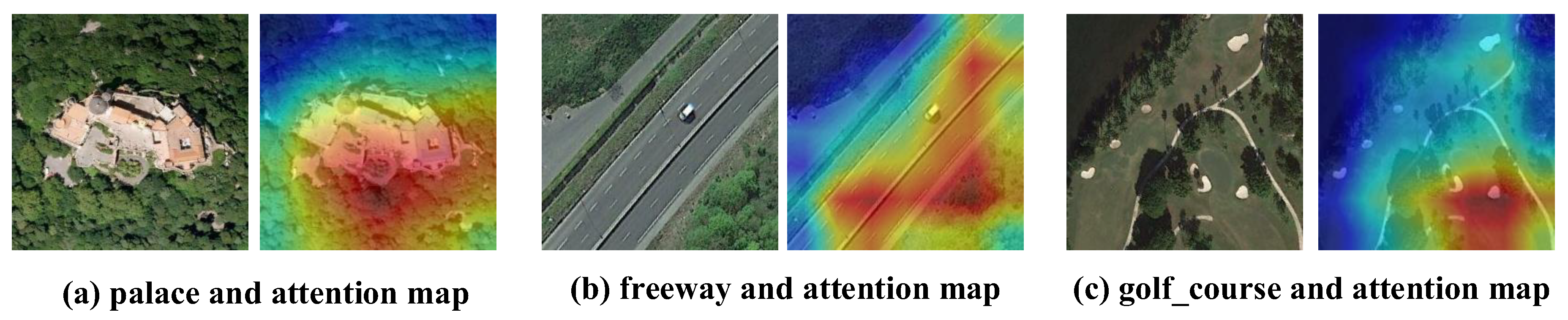
Figure 4 shows the sketch map of generating attention maps from all feature maps by weighting different channels of feature maps from the last convolutional layer of the fine-tuned ResNet18 model with a RELU function. As can be seen in Figure 4, the airplanes in airport class are considered as important objects. When training networks, the airplane in airport scenes may be laid with more emphasis, which may decrease the influence of redundant objects on extracting high-level features.
The feature fusion is an effective step in scene understanding task. In this section, we propose a simple and effective two-stream deep fusion architecture for remote scene classification. As shown in Figure 3(2), the first stream is called original RGB stream, which feeds original RGB images into the network. The second stream is named as saliency stream that applies the attention maps as an input. We designed the SFT network to extract valuable information from grey images.
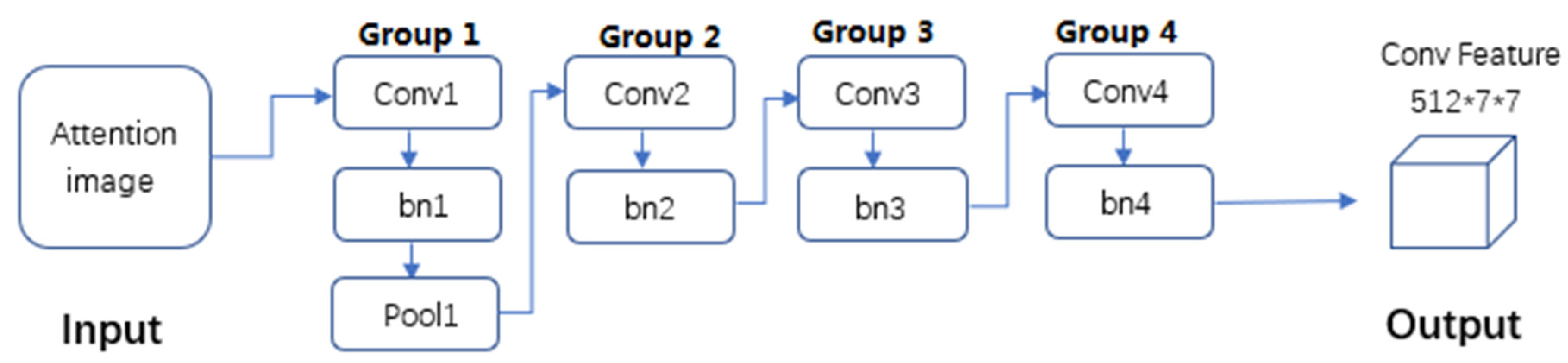
It is noteworthy that the two branches utilize different network structure, respectively, to extract features. The RGB stream is consistent with the ResNet-18 network structure since it has been proven to be effective in scene classification. The proposed SFT is used to extract features for attention maps. The architecture of SFT is presented in Figure 5 and the specific parameter settings of SFT are shown in Table 1. Two streams are both with an input of 224 × 224 × 3 and an output of 512 × 7 × 7. SFT contains 4 convolutional layers and 4 batch normalization layers, and one max-pooling layer is only used following the first convolutional layer. The first convolutional layer has 64 filters of size 7 × 7 with a stride of 2 pixels and padding with 3 pixels. The stride and padding of other convolutional layers are set as 2 and 1 pixel, respectively. The second, third, and fourth convolutional layers have 128, 256 and 512 filters with the size of 3 × 3, respectively. The batch normalization layers are consistent with the convolution kernel of the convolutional layer they are connected to. Max-pooling is carried out over a 3 × 3 window with stride 2. The batch normalization layers are aimed to reduce the possibility of overfitting when training the SFT architecture.
We used a spatial feature fusion strategy to fuse feature maps extracted from fine-tuned CNN models and proposed SFT model. In particular, we used multiplicative fusion functions (Equation (4)) for high-dimensional semantic feature fusion.
y d m u l = X i , j , d r g b × X i , j , d g r a d c a m
here, we denote X r g b as the output feature maps of the RGB stream with a size of 512 × 7 × 7. Similarly, X g r a d c a m is denoted as the output feature maps of the saliency stream with a size of 512 × 7 × 7. (i, j) is location of (7 × 7) feature maps and d is the channel number which ranges from 1 to 512. y d m u l is the feature maps after multiplicative fusion, and its dimension is still 512 × 7 × 7. .× represents the dot product of (7 × 7) feature maps from the RGB and saliency stream in each channel.
The multiplicative fusion can make the fused feature maps contain the sematic information from both the RGB and attention maps by operating dot product of (7 × 7) feature maps from the RGB and saliency stream in each channel. It can increase the discriminative ability of features extracted from scene images.

3.3. The Center-Based Cross Entropy Loss Function

While softmax loss function can help to effectively classify images, it is not enough to classify remote sensing images in a semantic way since feature representations of inner layers are similar for inter-class images. To improve the ability of feature representations to distinguish similar categories, we propose a new learning objective L t o t a l , which contains softmax loss function L s and center loss function L c . The formulation of L t o t a l can be formulated as Equation (5).
L t o t a l = L s + λ L c
As shown in [12], the scalar λ = 0.5 is used for balancing the two loss functions. The following part elaborates on softmax loss function and center loss functions. The softmax loss function L s is widely applied to classification of remote sensing images since it can ensure the convergence speed when the predicted values are close to true labels. The formulation of softmax loss function is shown in Equation (6).
L s = i = 1 m log e W y i T x i + b y i j = 1 n e W j T x i + b j
where x i d represents the features fused by multiplicative fusion for i-th image whose labels are y i b n denotes the learnt bias and W j d represents the j-th column of weights W d × n in the last fully connected layer. n represents the class number and m is the mini-batch size.
Although the softmax loss function may perform well under some circumstances, it ignores the influence of intra-class diversity on the loss function. Therefore, center loss function is introduced to the softmax loss function. The center loss function was proposed in [11] to minimize the intra-class variations while keeping the features of inter-class separable. The formulation of center loss function is shown in Equation (7).
L c = i = 1 m x i c u i 2 2 2
where x i d represents the features fused by multiplicative fusion for i-th image whose labels are y i c y i d represents centers calculated from features fused by multiplicative fusion belonging to y i -th class. 2 2 represents the square of L2-norm and m is the batch size of mini-batch.
The formulation of L t o t a l can reduce the influence of intra-class diversity on the loss function while maintaining the discriminative ability of fused features. If we backpropagate the network with the total loss function, the features with the same category will be close and those with diverse classes will be far away, which may decrease the possibility of confusion.

4. Experimental Results and Setup

4.1. Experimental Datasets and Setup

4.1.1. Description of Datasets

The proposed DDRL-AM approach is performed on four public datasets UC-Merced [23], NWPU-RESISC45 [10], AID [4], and a novel dataset EuroSAT [55] to verify the effectiveness and robustness of our proposed method.
(1)
UC Merced Dataset: The dataset includes 2100 aerial remote sensing images of 21 classes where each class contains 100 images. The size of the image, a pixel resolution of 0.3 m in the red green blue (RGB) color space, is 256 × 256 pixels. The dataset has a significant overlap among several classes, such as medium residential, dense residential, and sparse residential, which makes the dataset difficult for classification.
(2)
Aerial Image Dataset: It is a publicly available dataset that are segmented from large aerial imagery. It contains a total of 10,000 images and 30 aerial scene categories. This dataset is with about 200 to 400 samples of size 600 × 600 in each class.
(3)
NWPU-RESISC45 Dataset: This dataset includes a total of 31,500 remote sensing images divided into 45 scene classes. Each class consists of 700 images with a size of 256 × 256 pixels in the RGB color space. The range of spatial resolution is from about 30 to 0.2 m per pixel for most of the scene classes. This dataset contains more than 100 urban areas around the world. The high within class diversity and between-class similarity make the dataset more challenging.
(4)
EuroSAT Dataset: This dataset contains a total of 2700 scene images and 10 aerial scene categories. Unlike other aerial scene datasets, the dataset is challenging because the image size is very small for each category, where each image patch is 64 × 64 pixels.

4.1.2. Implementation Details

As mentioned above, at the first stage, we use the pre-trained ResNet [52] to produce attention maps consistent with the size of the original image. At the second stage, we experimented with the ResNet-18 architecture [52] and the SFT architecture that we designed to generate 512 × 7 × 7-dim feature tensors. We use the ADAM optimizer [56] with AMSGrad [57] where β1, β2, and c are equal to 0.9, 0.999, and 10 8 to optimize the center-based cross-entropy loss. The model is trained for 40 epochs. The DDRL-AM approach is implemented using the Pytorch framework [58]. This project used a GPU NVIDIA K40 for training and analysis.
In order to analyze the superiority of our proposed algorithm compared with other state-of-the-art algorithms, we need to ensure that the data split in this paper is the same as that in other compared approaches. Therefore, different training ratios are used for different datasets, which can better analyze the advantages and disadvantages of the method proposed in this paper. We randomly split the EuroSAT and UC Merced dataset into 80% for training and 20% for testing. For the NWPU-RESISC45 dataset, we set the ratios of the number of training set to 10% and 20% and the rest 90% and 80% for testing. For the AID dataset, two different training ratios 20% and 80% are set. Data augmentation is performed on the training images including original images and attention map, which are randomly rotated by 90°, 180°, 270°, horizontally flipped and vertically flipped.
Our proposed DDRL-AM method based on CNN models includes ResNet-18 and SFT architecture, which are detailed described in Section 3.1. In the end-to-end learning phase, the learning rate is set to 0.0001 for fine-tuned CNN model and 0.001 for SFT model and the classification layers. At the same time, we adopted the learning rate decay strategy. Every ten epochs for SFT model and the classification layers, the learning rate is reduced by γ = 0.1.

4.1.3. Evaluation Metrics

Overall accuracy and confusion matrix are two common quantitative evaluation metrics in image classification. The overall accuracy is defined as the number of correctly classified samples, without taking into account the type of category to which they belong, divided by the total number of samples. The confusion matrix is an informative table which is used to analyze the errors and confusions between different classes, and it count each class of correct and incorrect classification of the test images and accumulate the results in the table. At the same time, to obtain reliable results on all four datasets, we repeated the experiment 10 times for each training-test ratio, and then reported the mean and standard deviation of the results.

4.2. Comparison with State-of-the-Art Methods

We reported the mean scene classification accuracy (AC) and standard deviation (STD) of the proposed DDRL-AM methods. Several unsupervised feature learning based approaches including BoVW+SCK and CNN-based methods such as fine-tuned Inception V3, VGG19, and GoogLeNet, Deep CNN Transfer, Two-Stream Fusion, attention based residual network and so on, are considered as baseline methods in the UC Merced dataset.
Since the DDRL-AM use visual attention mechanisms to enrich the power of the CNN feature representations, we mainly compare our method with CNN feature-based methods including fine-tuned VGGNet-16+SVM [26], attention based residual network, multi-scale triplet loss, and D-CNNs [27] in the NWPU-RESISC45 dataset.
Table 2 and Table 3 show a baseline comparison on UC Merced and NWPU-RESISC45 datasets. Our approach provides superior performance with the lowest standard deviation compared with existing scene classification methods. BoVW, BoVW + SCK and SIFT + SC deliver poorer performance than CNN based methods since they may fail to extract high-level information from images. The proposed DDRL-AM framework performs better than Deep CNN Transfer, Two-Stream Fusion and so on, because it concentrates on salient regions of images in training a CNN and decrease the influence of between-class similarity and intra-class diversity.
Scene classification results of the proposed DDRL-AM framework on AID and EuroSAT datasets are shown in Table 4 and Table 5. For the AID and EuroSAT datasets, the proposed DDRL-AM framework is compared with several CNN-based scene classification methods such as CaffeNet, VGG-VD-16, GoogLeNet, ResNet-50 and so on. As we can see in Table 4 and Table 5, the proposed method outperforms other CNN-based methods with at least 2% accuracy. That is because attention maps can help to make the proposed DDRL-AM focus on the salient regions that can assist the scene classification. The DDRL-AM framework also shows higher stability compared with other CNN-based methods since it can increase the possibility of finding valuable information from input images and attention maps.

4.3. Statistical Histogram and Confusion Matrices

Furthermore, confusion matrices of four different datasets are plotted in Figure 6, Figure 7, Figure 8 and Figure 9 in order to analyze the performance of DDRL-AM framework in each land-cover type. It can be noted that the white spaces represent elements that are equal to zero. Each element(i,j) in the confusion matrix represents the ratio of test images belonging to land-cover type i but recognized as land-cover type j to the number of all test images.
From confusion matrix Figure 6, we can see that the classification accuracy of most classes are close to or even equal to 100% except for the airplane and freeways. That may be because some vehicles or airplanes share similar characteristics with backgrounds. By analyzing the confusion matrix on the NWPU-RESISIC45 dataset (Figure 7), we can further observe that the number of misclassified categories has been relatively reduced. The most notable confusion shown in Figure 7 is meadow and golf course, which may be caused by the fact that golf course’s area is too small and they may both contain a large area of green grass. Thus, meadow and golf course are easily confused. The church and sparse residential categories deliver poor performance since they are easily with categories that constitute the same objects but with diverse spatial distributions.
For the AID dataset (Figure 8), the proposed DDRL-AM framework achieves more than 90% accuracies in 27 categories. It delivers relatively low accuracy in square, resort, and school. That is because these may exist as the same salient object’s buildings in these three types of scenes but they have diverse spatial distributions. The proposed DDRL-AM framework may not distinguish the spatial distributions of these salient objects well.
The proposed DDRL-AM framework obtains accuracies more than 97% for each category in the EuroSAT dataset as we can see in Figure 9. That is because between-class similarity and within-class variance is relatively lower in this dataset compared with other three datasets. The proposed DDRL-AM framework can better reduce the between-class similarity and within-class variance for this dataset.

5. Discussion

5.1. Ablation Studies of Deep Discriminative Representation Learning with Attention Map (DDRL-AM) Approach

To verify the contribution of different modules in our DDRL framework, we compared three cases on different datasets. Three cases include (1) Resnet-18—our basic fine-tuning network for scene classification; (2) Resnet-18+AM—our two-stream feature fusion network with attention map (AM); (3) Resnet-18+AM+CL—our full DDRL model including center loss (CL).
We conducted experiments with four datasets and report the results in Table 6. We can see that: (1) The center loss and attention maps are both effective in increasing classification accuracy for each specific dataset since they can reduce the influence of within-class variance and unimportant regions on representing each image, respectively. (2) Compared with the center loss (CL) module, the feature fusion of the AM plays a more important role. That is because generated attention maps can better improve the discriminative power of deep visual features for scene classification.

5.2. Attention Maps Generated by the Gradient-Weighted Class Activation Mapping (Grad-CAM) Approach

The discriminative regions in images can indicate which area the network should focus on. The attention maps contain the information that various layers of the network can capture low-, mid-, and high-level representation features.
Figure 10 illustrates the attention maps from pre-trained ResNet-18 model by Grad-CAM [43] algorithm. From the RGB-saliency mask, it is clear that the fine-tuned network learns better to exploit information in regions corresponding to true labels and aggregate features from these salient regions. The attention maps essentially show where the spatial areas of input are that the network focuses on for making predictions. Note that the higher the brightness of the color is, the higher the importance of the corresponding area of the image is.

5.3. Visualization of Features Extracted from the Proposed DDRL-AM Method

Our approach treats Resnet-18 as a backbone architecture, which is a primary feature extractor. To explore and delve into the impact of different components on feature representation, we employed the t-SNE [63] algorithm to embed the high-dimensional features in 2-D space. We extracted 25088-dimensional features representations from the first fully connected layer, and we employed the t-SNE algorithm to embed the high-dimensional features in 2-D space for all scenes of the dataset. We separately visualized four datasets when the loss function is with and without center loss function, respectively. The visualization of features can be shown from Figure 11, Figure 12, Figure 13 and Figure 14.
By inspecting the derived clusters, it is clear that center-loss function can decrease the within-class diversity and inter-class similarity for each specific dataset such as harbor in UC Merced dataset, parking lot in NWPU-RESISC45 dataset, pond in the AID dataset, and Herbeceous Vegetation in the EuroSAT dataset. As we can see from Figure 11, Figure 12, Figure 13 and Figure 14, the center loss function makes all images that share similar semantic information closer in the feature space and features extracted from the DDRL-AM better distinguish images from different categories, which may lead to increased classification performance.

6. Conclusions

In this paper, we have proposed a novel method called DDRL-AM for remote sensing scene classification. We addressed the problem of class ambiguity by learning more discriminative features. Our approach involves two main tasks: (1) Building a two-stream architecture to fuse attention map semantic feature with original image semantic feature; (2) Training DDRL-AM that is coupled with a center-loss to obtain discriminative feature for remote sensing images. Extensive experiments were conducted on four benchmark remote sensing scene classification datasets.
Our results clearly show that our methods can achieve better results compared to the current state-of-the-art for remote sensing scene classification. Moreover, center loss and attention maps can help to increase classification performance. However, in this paper, we only investigated gradient-based localization method (Grad-CAM) generating the attention map. In the future, attention maps generated by manually designed algorithms that can explain the cnn’s mechanism will be investigated. Another future direction is based on our proposed method to evaluate heatmaps highlighting the image regions which bear the most responsibility for the prediction.

Author Contributions

Conceptualization, J.L. and D.L; investigation, J.L. and D.L.; methodology, J.L. and D.L.; validation, J.L. and D.L.; formal analysis, J.L.; visualization, J.L. and D.L.; writing–original draft preparation, J.L.; supervision, Y.W., G.X. and C.D.; writing–review and editing, J.L., D.L., Y.W., G.X., Y.Z., C.D. and Y.Z. All authors have read and agreed to the published version of the manuscript.

Funding

This research received no external funding.

Acknowledgments

The authors also would like to thank the anonymous reviewers. Last but not least, this paper is not the work of a single person but of a great team including members of Key Laboratory of Network Information System Technology.

Conflicts of Interest

The authors declare no conflict of interest.

References

  1. Blaschke, T. What’s wrong with pixels? Some recent developments interfacing remote sensing and GIS. Geobit/Gis 2001, 6, 12–17. [Google Scholar]
  2. Blaschke, T.; Lang, S.; Hay, G. Object-Based Image Analysis: Spatial Concepts for Knowledge-Driven Remote Sensing Applications; Springer Science & Business Media: Berlin, Germany, 2008. [Google Scholar]
  3. Gómez-Chova, L.; Tuia, D.; Moser, G.; Camps-Valls, G. Multimodal classification of remote sensing images: A review and future directions. Proc. IEEE 2015, 103, 1560–1584. [Google Scholar] [CrossRef]
  4. Xia, G.S.; Hu, J.; Hu, F.; Shi, B.; Bai, X.; Zhong, Y.; Zhang, L.; Lu, X. AID: A benchmark dataset for performance evaluation of aerial scene classification. IEEE Trans. Geosci. Remote. Sens. 2017, 55, 3965–3981. [Google Scholar] [CrossRef] [Green Version]
  5. Qi, K.; Wu, H.; Shen, C.; Gong, J. Land-use scene classification in high-resolution remote sensing images using improved correlatons. IEEE Geosci. Remote Sens. Lett. 2015, 12, 2403–2407. [Google Scholar] [CrossRef]
  6. Hu, F.; Xia, G.S.; Hu, J.; Zhang, L. Transferring deep convolutional neural networks for the scene classification of high-resolution remote sensing imagery. Remote. Sens. 2015, 7, 14680–14707. [Google Scholar] [CrossRef] [Green Version]
  7. Zou, Q.; Ni, L.; Zhang, T.; Wang, Q. Deep Learning Based Feature Selection for Remote Sensing Scene Classification. IEEE Geosci. Remote. Sens. Lett. 2015, 12, 2321–2325. [Google Scholar] [CrossRef]
  8. Dong, R.; Xu, D.; Jiao, L.; Zhao, J.; An, J. A Fast Deep Perception Network for Remote Sensing Scene Classification. Remote. Sens. 2020, 12, 729. [Google Scholar] [CrossRef] [Green Version]
  9. Pires de Lima, R.; Marfurt, K. Convolutional Neural Network for Remote-Sensing Scene Classification: Transfer Learning Analysis. Remote. Sens. 2020, 12, 86. [Google Scholar] [CrossRef] [Green Version]
  10. Cheng, G.; Han, J.; Lu, X. Remote sensing image scene classification: Benchmark and state of the art. Proc. IEEE 2017, 105, 1865–1883. [Google Scholar] [CrossRef] [Green Version]
  11. Vaswani, A.; Shazeer, N.; Parmar, N.; Uszkoreit, J.; Jones, L.; Gomez, A.N.; Kaiser, Ł.; Polosukhin, I. Attention is all you need. In Advances in Neural Information Processing Systems; Curran Associates: Long Beach, CA, USA, 2017; pp. 5998–6008. [Google Scholar]
  12. Wen, Y.; Zhang, K.; Li, Z.; Qiao, Y. A discriminative feature learning approach for deep face recognition. In European Conference on Computer Vision; Springer: Amsterdam, The Netherlands, 2016; pp. 499–515. [Google Scholar]
  13. Swain, M.J.; Ballard, D.H. Color indexing. Int. J. Comput. Vis. 1991, 7, 11–32. [Google Scholar] [CrossRef]
  14. Haralick, R.M.; Shanmugam, K. Textural features for image classification. IEEE Trans. Syst. ManCybern. 1973, 6, 610–621. [Google Scholar] [CrossRef] [Green Version]
  15. Jain, A.K.; Ratha, N.K.; Lakshmanan, S. Object detection using Gabor filters. Pattern Recognit. 1997, 30, 295–309. [Google Scholar] [CrossRef]
  16. Ojala, T.; Pietikainen, M.; Maenpaa, T. Multiresolution gray-scale and rotation invariant texture classification with local binary patterns. IEEE Trans. Pattern Anal. Mach. Intell. 2002, 24, 971–987. [Google Scholar] [CrossRef]
  17. Oliva, A.; Torralba, A. Modeling the shape of the scene: A holistic representation of the spatial envelope. Int. J. Comput. Vis. 2001, 42, 145–175. [Google Scholar] [CrossRef]
  18. Lowe, D.G. Distinctive image features from scale-invariant keypoints. Int. J. Comput. Vis. 2004, 60, 91–110. [Google Scholar] [CrossRef]
  19. Dalal, N.; Triggs, B. Histograms of oriented gradients for human detection. In Proceedings of the 2005 IEEE Computer Society Conference on Computer Vision and Pattern Recognition, San Diego, CA, USA, 20–25 June 2005; Volume 1, pp. 886–893. [Google Scholar]
  20. Fei-Fei, L.; Perona, P. A bayesian hierarchical model for learning natural scene categories. In Proceedings of the 2005 IEEE Computer Society Conference on Computer Vision and Pattern Recognition, San Diego, CA, USA, 20–25 June 2005; Volume 2, pp. 524–531. [Google Scholar]
  21. Jégou, H.; Douze, M.; Schmid, C.; Pérez, P. Aggregating local descriptors into a compact image representation. In Proceedings of the 2010 IEEE Computer Society Conference on Computer Vision and Pattern Recognition, San Francisco, CA, USA, 13–18 June 2010; pp. 3304–3311. [Google Scholar]
  22. Perronnin, F.; Sánchez, J.; Mensink, T. Improving the fisher kernel for large-scale image classification. In European Conference on Computer Vision; Springer: Heraklion, Crete, 2010; pp. 143–156. [Google Scholar]
  23. Lazebnik, S.; Schmid, C.; Ponce, J. Beyond bags of features: Spatial pyramid matching for recognizing natural scene categories. In Proceedings of the 2006 IEEE Computer Society Conference on Computer Vision and Pattern Recognition, New York, NY, USA, 17–22 June 2006; pp. 2169–2178. [Google Scholar]
  24. Yang, Y.; Newsam, S. Bag-of-visual-words and spatial extensions for land-use classification. In Proceedings of the 18th SIGSPATIAL International Conference on Advances in Geographic Information Systems; ACM: San Jose, CA, USA, 2010; pp. 270–279. [Google Scholar]
  25. Krizhevsky, A.; Sutskever, I.; Hinton, G.E. Imagenet classification with deep convolutional neural networks. In Advances in Neural Information Processing Systems; Curran Associates: Lake Tahoe, NV, USA, 2012; pp. 1097–1105. [Google Scholar]
  26. Russakovsky, O.; Deng, J.; Su, H.; Krause, J.; Satheesh, S.; Ma, S.; Huang, Z.; Karpathy, A.; Khosla, A.; Bernstein, M. Imagenet large scale visual recognition challenge. Int. J. Comput. Vis. 2015, 115, 211–252. [Google Scholar] [CrossRef] [Green Version]
  27. Wang, Y.; Zhang, L.; Deng, H.; Lu, J.; Huang, H.; Zhang, L.; Liu, J.; Tang, H.; Xing, X. Learning a discriminative distance metric with label consistency for scene classification. IEEE Trans. Geosci. Remote. Sens. 2017, 55, 4427–4440. [Google Scholar] [CrossRef]
  28. Cheng, G.; Yang, C.; Yao, X.; Guo, L.; Han, J. When deep learning meets metric learning: Remote sensing image scene classification via learning discriminative CNNs. IEEE Trans. Geosci. Remote. Sens. 2018, 56, 2811–2821. [Google Scholar] [CrossRef]
  29. Penatti, O.A.; Nogueira, K.; dos Santos, J.A. Do deep features generalize from everyday objects to remote sensing and aerial scenes domains? In Proceedings of the IEEE Conference on Computer Vision and Pattern Recognition Workshops; IEEE: Boston, MA, USA, 2015; pp. 44–51. [Google Scholar]
  30. Castelluccio, M.; Poggi, G.; Sansone, C.; Verdoliva, L. Land use classification in remote sensing images by convolutional neural networks. arXiv 2015, arXiv:1508.00092. [Google Scholar]
  31. Zhang, L.; Zhang, L.; Du, B. Deep learning for remote sensing data: A technical tutorial on the state of the art. IEEE Geosci. Remote. Sens. Mag. 2016, 4, 22–40. [Google Scholar] [CrossRef]
  32. Itti, L.; Koch, C.; Niebur, E. A model of saliency-based visual attention for rapid scene analysis. IEEE Trans. Pattern Anal. Mach. Intell. 1998, 20, 1254–1259. [Google Scholar] [CrossRef] [Green Version]
  33. Zhou, Y.; Zhu, Y.; Ye, Q.; Qiu, Q.; Jiao, J. Weakly Supervised Instance Segmentation using Class Peak Response. arXiv 2018, arXiv:1804.00880. [Google Scholar]
  34. Wei, Y.; Feng, J.; Liang, X.; Cheng, M.M.; Zhao, Y.; Yan, S. Object region mining with adversarial erasing: A simple classification to semantic segmentation approach. IEEE CVPR 2017, 1, 3. [Google Scholar]
  35. Zhang, J.; Bargal, S.A.; Lin, Z.; Brandt, J.; Shen, X.; Sclaroff, S. Top-down neural attention by excitation backprop. Int. J. Comput. Vis. 2018, 126, 1084–1102. [Google Scholar] [CrossRef] [Green Version]
  36. Jetley, S.; Lord, N.A.; Lee, N.; Torr, P.H. Learn to pay attention. arXiv 2018, arXiv:1804.02391. [Google Scholar]
  37. Wang, F.; Jiang, M.; Qian, C.; Yang, S.; Li, C.; Zhang, H.; Wang, X.; Tang, X. Residual attention network for image classification. arXiv 2017, arXiv:1704.06904. [Google Scholar]
  38. Woo, S.; Park, J.; Lee, J.Y.; Kweon, I.S. Cbam: Convolutional block attention module. In Proceedings of the European Conference on Computer Vision; Springer: Munich, Germany, 2018. [Google Scholar]
  39. Park, J.; Woo, S.; Lee, J.Y.; Kweon, I.S. BAM: Bottleneck attention module. arXiv 2018, arXiv:1807.06514. [Google Scholar]
  40. Hu, J.; Shen, L.; Sun, G. Squeeze-and-excitation networks. arXiv 2017, arXiv:1709.01507. [Google Scholar]
  41. Nakka, K.K.; Salzmann, M. Deep Attentional Structured Representation Learning for Visual Recognition. arXiv 2018, arXiv:1805.05389. [Google Scholar]
  42. Xu, R.; Tao, Y.; Lu, Z.; Zhong, Y. Attention-mechanism-containing neural networks for high-resolution remote sensing image classification. Remote. Sens. 2018, 10, 1602. [Google Scholar] [CrossRef] [Green Version]
  43. Chen, J.; Wang, C.; Ma, Z.; Chen, J.; He, D.; Ackland, S. Remote sensing scene classification based on convolutional neural networks pre-trained using attention-guided sparse filters. Remote. Sens. 2018, 10, 290. [Google Scholar] [CrossRef] [Green Version]
  44. Bi, Q.; Qin, K.; Li, Z.; Zhang, H.; Xu, K.; Xia, G.S. A Multiple-Instance Densely-Connected ConvNet for Aerial Scene Classification. IEEE Trans. Image Process. 2020, 29, 4911–4926. [Google Scholar] [CrossRef] [PubMed]
  45. Cao, R.; Fang, L.; Lu, T.; He, N. Self-Attention-Based Deep Feature Fusion for Remote Sensing Scene Classification. IEEE Geosci. Remote. Sens. Lett. 2020. [Google Scholar] [CrossRef]
  46. Guo, Y.; Ji, J.; Lu, X.; Huo, H.; Fang, T.; Li, D. Global-local attention network for aerial scene classification. IEEE Access 2019, 7, 67200–67212. [Google Scholar] [CrossRef]
  47. Wang, J.; Shen, L.; Qiao, W.; Dai, Y.; Li, Z. Deep feature fusion with integration of residual connection and attention model for classification of VHR remote sensing images. Remote. Sens. 2019, 11, 1617. [Google Scholar] [CrossRef] [Green Version]
  48. Wang, Q.; Liu, S.; Chanussot, J.; Li, X. Scene classification with recurrent attention of VHR remote sensing images. IEEE Trans. Geosci. Remote. Sens. 2018, 57, 1155–1167. [Google Scholar] [CrossRef]
  49. Simonyan, K.; Zisserman, A. Two-stream convolutional networks for action recognition in videos. In Advances in Neural Information Processing Systems; Curran Associates: Montréal, QC, Canada, 2014; pp. 568–576. [Google Scholar]
  50. Feichtenhofer, C.; Pinz, A.; Zisserman, A. Convolutional two-stream network fusion for video action recognition. In Proceedings of the IEEE Conference on Computer Vision and Pattern Recognition; IEEE: Las Vegas, NV, USA, 2016; pp. 1933–1941. [Google Scholar]
  51. Chaib, S.; Liu, H.; Gu, Y.; Yao, H. fusion for VHR remote sensing scene classification. IEEE Trans. Geosci. Remote. Sens. 2017, 55, 4775–4784. [Google Scholar] [CrossRef]
  52. He, K.; Zhang, X.; Ren, S.; Sun, J. Deep residual learning for image recognition. In Proceedings of the IEEE Conference on Computer Vision and Pattern Recognition; IEEE: Las Vegas, NV, USA, 2016; pp. 770–778. [Google Scholar]
  53. Selvaraju, R.R.; Cogswell, M.; Das, A.; Vedantam, R.; Parikh, D.; Batra, D. Grad-CAM: Visual Explanations from Deep Networks via Gradient-Based Localization. In Proceedings of the IEEE International Conference on Computer Vision; IEEE: Venice, Italy, 2017; pp. 618–626. [Google Scholar]
  54. Zeiler, M.D.; Fergus, R. Visualizing and Understanding Convolutional Networks. In European Conference on Computer Vision; Springer: Zurich, Switzerland, 2014; pp. 818–833. [Google Scholar]
  55. Helber, P.; Bischke, B.; Dengel, A.; Borth, D. Eurosat: A novel dataset and deep learning benchmark for land use and land cover classification. arXiv 2017, arXiv:1709.00029. [Google Scholar]
  56. Kingma, D.P.; Ba, J. Adam: A method for stochastic optimization. arXiv 2014, arXiv:1412.6980. [Google Scholar]
  57. Reddi, S.J.; Kale, S.; Kumar, S. On the Convergence of Adam and Beyond. arXiv 2014, arXiv:1904.09237. [Google Scholar]
  58. Paszke, A.; Gross, S.; Massa, F.; Lerer, A.; Bradbury, J.; Chanan, G.; Killeen, T.; Lin, Z.; Gimelshein, N.; Antiga, L.; et al. PyTorch: An imperative style, high-performance deep learning library. In Advances in Neural Information Processing Systems; Curran Associates: Vancouver, BC, Canada, 2019; pp. 8024–8035. [Google Scholar]
  59. Cheriyadat, A.M. Unsupervised feature learning for aerial scene classification. IEEE Trans. Geosci. Remote. Sens. 2014, 52, 439–451. [Google Scholar] [CrossRef]
  60. Yu, Y.; Liu, F. A Two-Stream Deep Fusion Framework for High-Resolution Aerial Scene Classification. Comput. Intell. Neurosci. 2018, 2018, 8639367. [Google Scholar] [CrossRef] [PubMed] [Green Version]
  61. Fan, R.; Wang, L.; Feng, R.; Zhu, Y. Attention based Residual Network for High-Resolution Remote Sensing Imagery Scene Classification. In IGARSS 2019–2019 IEEE International Geoscience and Remote Sensing Symposium; IEEE: Yokohama, Japan, 2019; pp. 1346–1349. [Google Scholar]
  62. Zhang, J.; Lu, C.; Wang, J.; Yue, X.G.; Lim, S.J.; Al-Makhadmeh, Z.; Tolba, A. Training Convolutional Neural Networks with Multi-Size Images and Triplet Loss for Remote Sensing Scene Classification. Sensors 2020, 20, 1188. [Google Scholar] [CrossRef] [PubMed] [Green Version]
  63. Maaten, L.V.D.; Hinton, G. Visualizing data using t-SNE. J. Mach. Learn. Res. 2008, 4629, 2579–2605. [Google Scholar]
Figure 1. Three major challenges: (a) large intra-class variations; (b) small inter-class dissimilarity; (c) diverse objects in scene images. These examples come from the challenging NWPU-RESISC45 dataset [10].
Remotesensing 12 01366 g001
Figure 2. Attention maps of three categories generated by Gradient-weighted Class Activation Mapping (Grad-CAM) algorithm. The attention maps have high responses localized at the area related to true semantic labels.
Remotesensing 12 01366 g002
Figure 3. Overview of our framework, which is comprised of (a) convolutional neural networks (CNN) pretrained on ImageNet and fine-tuned on training dataset and Grad-CAM architecture to generate discriminative attention map, and (b) a two-stream architecture to fuse high-level features extracted from original image and attention maps and combine multiple loss functions. For simplicity, the different color block represents different network structure layers, respectively.
Remotesensing 12 01366 g003
Figure 4. Attention mapping over conv_5 feature maps from fine-tuned resnet-18 model.3.3. Feature Fusion.
Remotesensing 12 01366 g004
Figure 5. Spatial Feature Transformer Architecture. Conv and pool represent the convolutional and pooling layers. Bn is the batch normalization layer.
Remotesensing 12 01366 g005
Figure 6. Confusion matrices of the UC Merced dataset under the training ratio of 80% using Deep Discriminative Representation Learning with Attention Map (DDRL-AM). The results in Figure 6 correspond to results shown in Table 2.
Remotesensing 12 01366 g006
Figure 7. Confusion matrices of the NWPU-RESISC45 dataset under the training ratio of 80% using DDRL-AM. The results in Figure 7 correspond to results shown in Table 3.
Remotesensing 12 01366 g007
Figure 8. Confusion matrices of the DDRL-AM framework with 80% training data of AID. The results in Figure 8 correspond to results shown in Table 4.
Remotesensing 12 01366 g008
Figure 9. Confusion matrices of DDRL-AM framework with 80% training data of EuroSAT. The results in Figure 9 correspond to results shown in Table 5.
Remotesensing 12 01366 g009
Figure 10. Saliency mask results. The Grad-CAM visualization is calculated for the last convolutional layers. Each input image is shown in the first line, where saliency images and attention maps are shown in the second and third line, respectively.
Remotesensing 12 01366 g010
Figure 11. 2-D scatterplots of high-dimensional features generated with t-SNE over the UC Merced dataset. (left) without center-loss function. (right) with center-loss function.
Remotesensing 12 01366 g011
Figure 12. 2-D scatterplots of high-dimensional features generated with t-SNE over the NWPU-RESISC45 dataset. (left) without center-loss function. (right) with center-loss function.
Remotesensing 12 01366 g012
Figure 13. 2-D scatterplots of high-dimensional features generated with t-SNE over the AID dataset. (left) without center-loss function. (right) with center-loss function.
Remotesensing 12 01366 g013
Figure 14. 2-D scatterplots of high-dimensional features generated with t-SNE over the EuroSAT dataset. (left) without center-loss function. (right) with center-loss function.
Remotesensing 12 01366 g014
Table 1. Spatial Feature Transformer (SFT) Architecture Parameter Setting.
Architecture Group1 Group2Group3Group4
Conv1 (k_num/k_size/s/p)BN1 (k_num/mom)Maxpool1 (k_size/s/p)Conv2 (k_num/k_size/s/p)BN2 (k_num/mom)Conv3 (k_num)BN3 (k_num)Conv4 (k_num)BN4 (k_num)
Parameter64/7 × 7/2 × 2/3 × 364/0.13 × 3/2/1128/3 × 3/2 × 2/1 × 1128/0.1256256512512
Table 2. Scene classification results (ac% ± std) using the UC merced dataset with 80% training ratio.
MethodsAccuracy and Standard Deviation
BoVW [23]76.81
BoVW + SCK [23]77.71
SIFT + SC [58]81.67
Unsupervised feature learning [59]81.67 ± 1.23
Fine-tuned GoogLeNet [30]97.10
Deep CNN Transfer [6]98.49
Fusion by addition [50]97.42 ± 1.79
Two-Stream Fusion [60]98.02 ± 1.03
D-CNN with VGGNet-16 [27]98.93 ± 0.10
Fine-tuned Inception V3 [9]98.3
Fine-tuned VGG19 [9]98.1
Attention based Residual Network [61]98.81 ± 0.30
DDRL-AM (ours)99.05 ± 0.08
Table 3. Scene classification results (ac% ± std) using the nwpu-resisc45 dataset.
Methods10% Training Ratio20% Training Ratio
Fine-tuned VGGNet-16 [26]87.15 ± 0.4590.36 ± 0.18
D-CNN with VGGNet-16 [27]89.22 ± 0.5091.89 ± 0.22
Attention based Residual Network [61]-92.10 ± 0.30
Multi-scale triplet loss [62]88.30 ± 0.2491.62 ± 0.35
DDRL-AM (ours)92.17 ± 0.0892.46 ± 0.09
Table 4. Scene classification results (ac% ± std) using the AID dataset.
Methods80% Training Ratio20% Training Ratio
CaffeNet89.53 ± 0.3186.86 ± 0.45
VGG-VD-1689.64 ± 0.3686.59 ± 0.29
GoogLeNet86.39 ± 0.5583.44 ± 0.40
Fine-tuned Inception V395.0-
Fine-tuned VGG1993.6-
Multi-scale triplet loss92.65 ± 0.29-
DDRL-AM (ours)96.25 ± 0.0592.36 ± 0.10
Table 5. Scene classification results (ac% ± std) using the EuroSAT dataset with 80% training ratio.
MethodsAccuracy and Standard Deviation
CNN (two layers)87.96
ResNet-5096.43
GoogleNet96.02
DDRL-AM (ours)98.74 ± 0.05
Table 6. Ablation study results (%) for our DDRL-AM model on different datasets.
DatasetComponentsAccuracyΔ
UC Merced–80%ResNet-1896.19
ResNet-18 + AM98.242.05
ResNet-18 + AM+CL99.052.86
NWPU-RESISC 45–20%ResNet-1890.11
ResNet-18 + AM91.030.92
ResNet-18 + AM+CL92.462.35
NWPU-RESISC 45–10%ResNet-1890.01
ResNet-18 + AM91.841.83
ResNet-18 + AM+CL92.172.16
AID–20%ResNet-1886.15
ResNet-18 + AM91.195.04
ResNet-18 + AM+CL92.366.21
AID–80%ResNet-1892.85
ResNet-18 + AM95.903.05
ResNet-18 + AM+CL96.253.40
EuroSAT–80%ResNet-1897.52
ResNet-18 + AM98.500.98
ResNet-18 + AM+CL98.741.22

