Soil Moisture–Vegetation–Carbon Flux Relationship under Agricultural Drought Condition using Optical Multispectral Sensor

Abstract

Agricultural drought is triggered by a depletion of moisture content in the soil, which hinders photosynthesis and thus increases carbon dioxide (CO₂) concentrations in the atmosphere. The aim of this study is to analyze the relationship between soil moisture (SM) and vegetation activity toward quantifying CO₂ concentration in the atmosphere. To this end, the MODerate resolution imaging spectroradiometer (MODIS), an optical multispectral sensor, was used to evaluate two regions in South Korea for validation. Vegetation activity was analyzed through MOD13A1 vegetation indices products, and MODIS gross primary productivity (GPP) product was used to calculate the CO₂ flux based on its relationship with respiration. In the case of SM, it was calculated through the method of applying apparent thermal inertia (ATI) in combination with land surface temperature and albedo. To validate the SM and CO₂ flux, flux tower data was used which are the observed measurement values for the extreme drought period of 2014 and 2015 in South Korea. These two variables were analyzed for temporal variation on flux tower data as daily time scale, and the relationship with vegetation index (VI) was synthesized and analyzed on a monthly scale. The highest correlation between SM and VI (correlation coefficient (r) = 0.82) was observed at a time lag of one month, and that between VI and CO₂ (r = 0.81) at half month. This regional study suggests a potential capability of MODIS-based SM, VI, and CO₂ flux, which can be applied to an assessment of the global view of the agricultural drought by using available satellite remote sensing products.

1. Introduction

Several decades of recent climate change are mainly driven by anthropogenic influences in a global scale. Even with the significant societal impact of the drought, it still remains challenging to define its causes and effects of the drought in the context of hydrological and agricultural practices. Recent studies demonstrate that drought can be classified into various types based on the theoretical definitions [1,2,3,4,5]. Agricultural drought is one of the main drought classifications. In this agricultural drought, short-term rainfall deficit decreases soil moisture (hereafter SM) and affects vegetation activity [6,7]. Most previous studies estimated the drought index using SM or the vegetation index (hereafter VI), to analyze agricultural drought [6,7,8,9,10,11,12,13,14]. For example, Kogan derived the vegetation health index (VHI) and the vegetation condition index (hereafter VCI) from the VI [8]. Keshavarz et al. derived the soil wetness deficit index (hereafter SWDI) from SM [11]. Most of the recent studies used remote sensing data as the alternative to indirectly estimate SM and VI.

Among the agricultural drought-related factors, VIs can be determined by optical sensor products. Among the VIs, the normalized difference vegetation index (NDVI) and the enhanced vegetation index (EVI) provided by the moderate resolution imaging spectroradiometer (MODIS) are widely used [15,16,17,18]. Generally, satellite-based soil moisture is commonly used as detected by passive microwave sensors. Soil moisture calculated in the frequency range of L-, X-, and C-bands of microwave sensors has been applied in many studies [19,20,21,22,23]. SM based on passive microwaves has high accuracy, while spatial resolution is relatively coarse. These SM products are suitable for analyzing large areas, such as a continent, but not catchments or smaller regions. In order to overcome spatial limitations and pursue high-resolution data of smaller regions, an SM estimation method that uses optical sensors has been explored [24,25,26,27]. This optics-based method is based on the relationship between land surface temperature (hereafter LST) and land surface albedo. With this approach, the SM at 0.5-km spatial resolution can be calculated in accordance with LST and albedo. In addition, most studies related to agricultural drought have derived drought indices using SM and VI and by monitoring and analyzing agricultural drought status or analyzed the relationship between vegetation activity and photosynthesis [28,29,30]. However, few studies have analyzed the inter-relationship among SM, VI, and photosynthesis. This study aims to analyze the relationship between a surface flux and a vegetation phenology, under extreme climates such as drought. Based on data available in the literature, we hypothesize that prolonged periods of agricultural drought cause vegetation to become inactive and thus hamper photosynthesis. This in turn increases the amount of CO₂ in the atmosphere. As part of the research objectives, we provide evidence for this hypothesis and validate it.

To show the evidence of the CO₂ increase due to the recent agricultural drought, the main parts of this study are as follows: (a) to evaluate the applicability of optical sensor-derived SM by comparing the MODIS data-derived SM (an optical multispectral sensor) with the SM observed in a flux tower; (b) to examine the possibility of remote sensing-based carbon monitoring by estimating CO₂ flux through gross primary productivity (hereafter GPP), a MODIS product, and compare it with the results observed in the flux tower; and, (c) to verify the hypothesis that prolonged periods of agricultural drought reduce SM, hinder vegetation growth, hamper photosynthesis and thus increase CO₂ concentrations. In particular, in order to analyse the effects of soil moisture, vegetation, and CO2 under drought condition, lag correlation analysis was performed between factors synthesized as a monthly scale. It is intended to understand how sequential changes between factors occur in extreme climatic conditions. There have been many studies on the impact analysis of the factors interacting between the land surface and the atmosphere—but few studies for agricultural perspectives. This study is expected to show the interaction relationship between the atmosphere and the land surface under extreme climatic conditions such as agricultural drought.

2. Materials and Methods

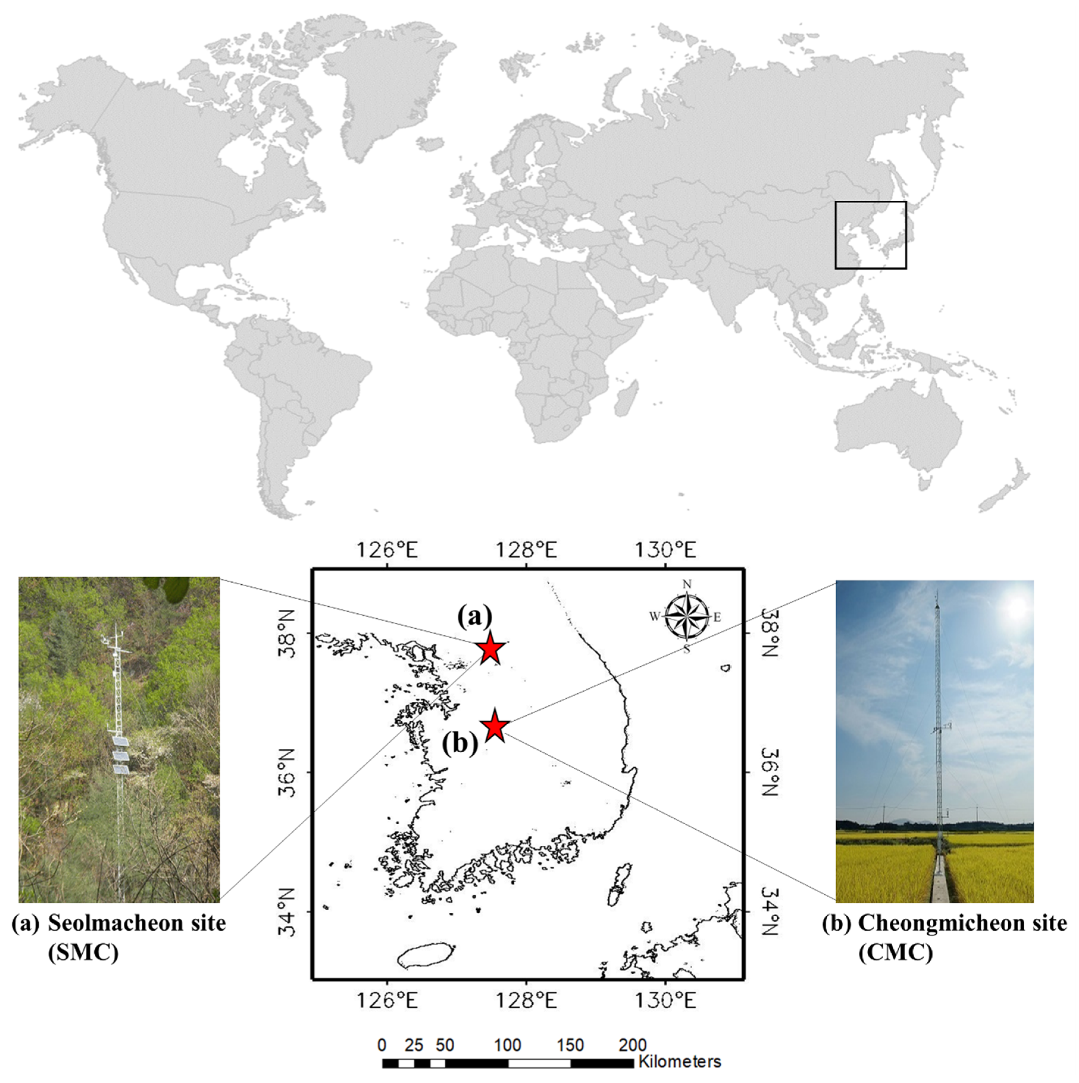
2.1. Study Area

South Korea the study area of this research, is located at a latitude of 33–39°N and a longitude of 124–131°E (Figure 1). According to the International Geosphere-Biosphere Programme (IGBP) land cover classification, the landmass of South Korea consists of mixed forests (40%), croplands (30%), deciduous broadleaf forests (14%), woody savannas (6%), and urban and built-up areas (5%) [7,31]. Western South Korea is mostly composed of croplands, while the central and east parts are covered with mixed and deciduous broadleaf forests. To validate the estimated remote sensing-based CO₂ flux and SM, CO₂ flux and SM data of the Sulmacheon (hereafter SMC) and Cheongmicheon (hereafter CMC) flux tower were provided by the Korea Institute of Hydrological Survey. The SMC flux tower is in Jeokseong-myeon, Paju-si, Gyeonggi-do, and the area is a typical mountainous terrain located at an altitude of 293 m.a.s.l. The CMC flux tower is in Janghowon-eup, Icheon-si, Gyeonggi-do, and is composed of a rice paddy terrain (

Table 1. Characteristics of the selected sites in study area.

Site	Latitude (°N)	Longitude (°E)	Altitude (m)	Land Cover	LAI	Terrain
Cheonmicheon (CMC)	37.16	127.65	141	Rice Paddy	1–2	Flat
Sulmacheon (SMC)	37.94	126.95	293	Mixed Forest	6–8	Mountainous

). Data in the flux tower is measured by the Eddy covariance method, and reliable data is provided by quality control [30]. Both the CO₂ flux and SM data used in this study were extracted every 30 min, and data from 2014 and 2015 were used to analyze the relationship between the variables during a period of extreme drought status in Korea.

2.2. Optical Multispectral Sensor Dataset

We used MODIS data to calculate SM, VI, and GPP (

Table 2. Remote sensing data used in this study.

Product ID	Product	Spatial Resolution (km)	Temporal Resolution
MOD11A1	Land surface temperature	0.5	Daily
MCD12Q1	Land cover	0.5	Yearly
MOD13A1	Vegetation indices	0.5	16 days
MOD17A2H	Gross primary productivity	0.5	8 days
MCD43A3	Albedo	0.5	Daily

). First, SM was calculated using LST of MOD11A1 and land surface albedo of MCD43A3. The details are introduced in Section 2.4. For VI, we used the NDVI of MOD13A1 and analyzed the CO₂ generation according to vegetation activity through GPP of MOD17A2H. A method for CO₂ analysis using GPP is introduced in Section 2.3. All MODIS data used in this study had a spatial resolution of 0.5 km × 0.5 km. As for the temporal resolution, MOD11A1 and MCD43A3 data were provided daily; MOD17A2H eight days, and MOD13A1 16 days. Various MODIS land products have different temporal resolutions. As these products were combined to calculate the drought index, they must be unified using the same time frame. Temporal resolution is unified on a daily scale. For the eight-day product, the same value is matched for the remaining seven days from the starting point. Similarly, the 16-day product matches the same value for the remaining 15 days from the starting point. All MODIS data from 2001 to 2019 can be obtained from NASA Earthdata website [32]. For this study, the results were obtained for 2001 to 2015.

2.3. Calculation of CO₂ Flux

Since CO₂ cannot be mapped directly by satellite images, it is calculated through the relationship between CO₂ and GPP. In general, CO₂ in the atmosphere is generated through the following three processes. First, through vegetation activity, i.e., the process of absorbing CO₂ in the atmosphere and producing oxygen (photosynthesis). Second, the process of vegetation biomass maintenance. Third, respiration according to dependent nutrition. Plants have a bidirectional flux that absorbs CO₂ from the atmosphere through photosynthesis and recirculates part of it to the atmosphere through respiration. The total amount of organic matter produced by plants by absorbing CO₂ through photosynthesis, or the total amount of carbon generated through the CO₂ circulation in the atmosphere, which is called GPP. Amid these processes, the relationship between CO₂ and GPP can be expressed by the following equation.

NEE = R_e − GPP,

(1)

where NEE, (net ecosystem exchange) is a measure of the net exchange of carbon between an ecosystem and the atmosphere and is a primary measurement of the ecosystem’s carbon sink strength [33,34,35,36]. R_e is the ecosystem respiration of plants. NEE is the CO₂ flux data measured in the flux tower applied in this study. The relationship between CO₂ flux and GPP can be calculated from the Re value. Re is calculated by the following Equation [37];

$${\mathrm{R}}_{\mathrm{e}}{=\mathrm{R}}_{\mathrm{ref}}{\exp (\mathrm{E}}_0\left[\frac{1}{{\mathrm{T}}_{\mathrm{ref}}{-\mathrm{T}}_0} -\frac{1}{{\mathrm{T}}_{\mathrm{a}}{-\mathrm{T}}_0}\right]),$$

(2)

where R_ref is the reference ecosystem respiration, T_ref the reference temperature (10 °C), E₀ the activation energy, T₀ −46.02 °C, and T_a the air temperature. R_ref and E₀ are the empirical constants obtained by regression with the air temperature [37].

2.4. Measurement of Soil Moisture Content by Optical Multispectral Sensor

Previous studies have estimated SM using passive microwave sensors by observing the brightness temperature of a land surface through sensors and leveraging its relationship with temperature. Since SM is calculated according to the physical properties of the land surface, it is quite accurate. However, it has a coarser spatial resolution than the optical sensor. The total area of South Korea is 106,286 km². Since the AMSR-based SM products have a spatial resolution of 25 km, the entire country could be represented in 170 pixels only. Because the 0.5-km-resolution product of the optical sensor can represent the area with approximately 425,000 pixels, the passive microwave sensor product faces limitations in analyzing physical properties for cases such as this study. To overcome the limitations, we applied a method for calculating volumetric SM using optical sensor products presented by Verstraeten et al. [24]. The optical sensor used in this study is MODIS. Specifically, MOD11A1 LST and MOD43A3 land surface albedo were used.

$$\Delta {\mathrm{LST}=\mathrm{LST}}_{\mathrm{daytime}} {- \mathrm{LST}}_{\mathrm{nighttime}},$$

(3)

$$\mathrm{ATI}=\frac{1 - \mathsf{\alpha }}{\Delta \mathrm{LST}},$$

(4)

$$\mathrm{SM}=\frac{{\mathrm{ATI}}_{\mathrm{i}}{ - \mathrm{ATI}}_{\min }}{{\mathrm{ATI}}_{\max }{ - \mathrm{ATI}}_{\min }},$$

(5)

where ΔLST is the difference between LST_daytime and LST_nighttime, LST_daytime is the land surface temperature during daytime, and LST_nighttime is the temperature during nighttime. ATI, which stands for apparent thermal inertia, is a physical property of materials describing their impedance to temperature change. α is the land surface albedo and 1- α represents physically absorbance. Volumetric SM (m³ m⁻³) can be calculated by normalizing the maximum and minimum ATI values.

2.5. Agricultural Drought Indices

For a period of drought, the relationship between soil moisture, vegetation activity, and carbon generation were analyzed by the drought indices vegetation condition index (VCI) and the standardized soil moisture index (SSMI).

2.5.1. Vegetation Condition Index (VCI)

VI was used to analyze agricultural drought. VCI was calculated by normalizing the NDVI provided by MOD13A1 of the MODIS sensor [8].

$$\mathrm{VCI}=\frac{{\mathrm{NDVI}}_{\mathrm{i}}{ - \mathrm{NDVI}}_{\min }}{{\mathrm{NDVI}}_{\max }{ - \mathrm{NDVI}}_{\min }}.$$

(6)

VCI compares the current NDVI to those observed during the same period in previous years. It is expressed in % and gives an estimate of the location of the observed value between the extrema (minimum and maximum values) in the previous years.

2.5.2. Standardized Soil Moisture Index (SSMI)

In order to analyze the agricultural drought condition, a standard normalization was performed on the volumetric SM introduced in Section 2.4, and the result was processed as an index. This index is named standardized soil moisture index (SSMI). The SSMI is calculated as follows.

$$\mathrm{SSMI}=\mathrm{Z}(\frac{{\mathrm{SM}}_{\mathrm{i}}{ - \mathrm{SM}}_{\min }}{{\mathrm{SM}}_{\max }{ - \mathrm{SM}}_{\min }}),$$

(7)

where Z is the standardized normalization, SM_max the maximum SM value, SM_min the minimum SM value, and SM_i the SM in the i-th time point.

3. Results and Discussion

3.1. Comparative Analysis of Optical Sensor Products and In Situ Data

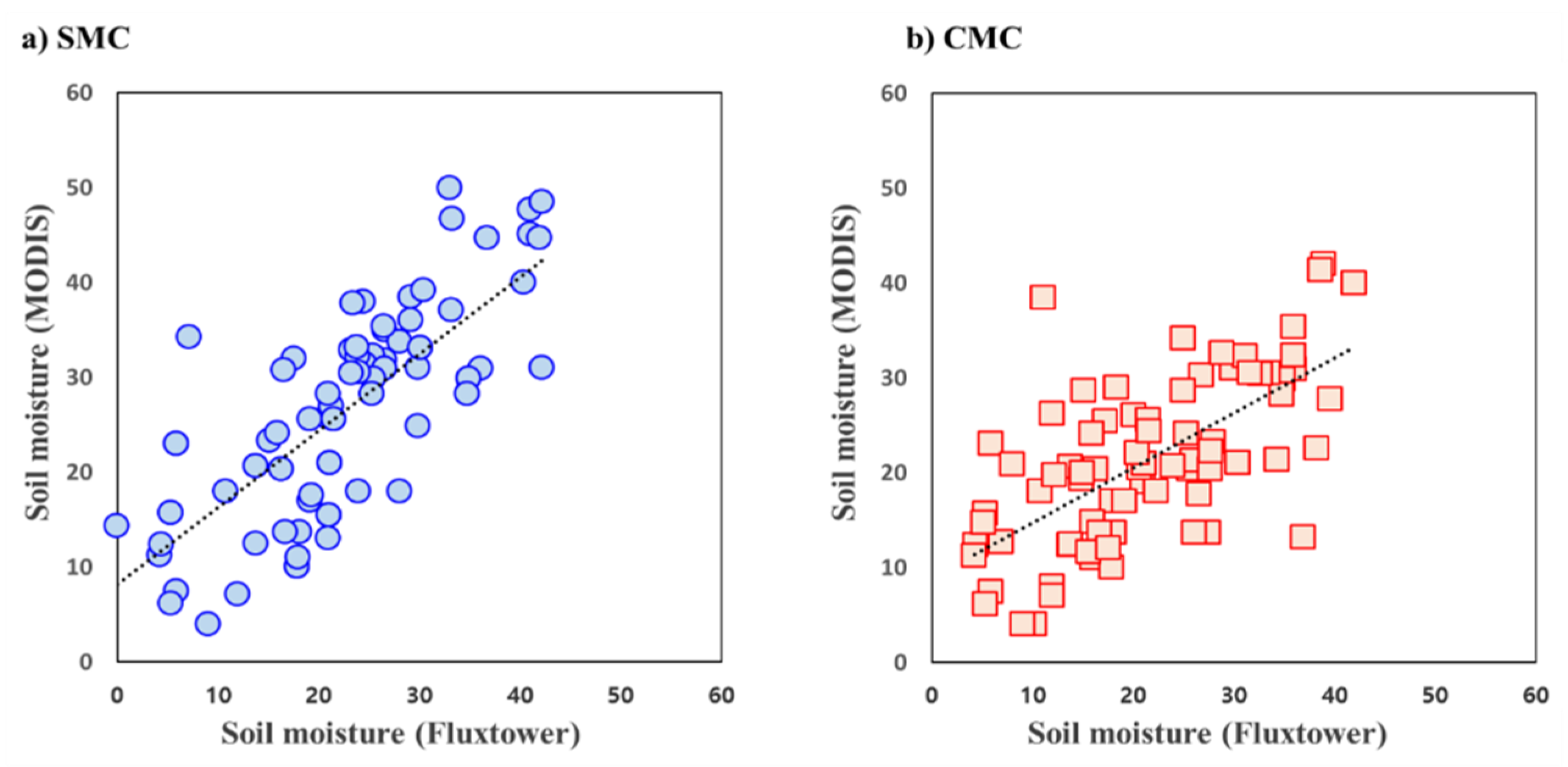
3.1.1. Temporal Variations of Soil Moisture and Comparison with Ground Observation

As mentioned in Section 2.4, Verstraeten et al. [24] and Chang et al. [25] presented a method for soil moisture (SM) estimation using optical sensor products. In this study, SM was calculated based on this estimation method (hereinafter referred to as SM_MODIS) and compared with soil moisture (hereinafter referred to as SM_fluxtower) measured at the SMC and CMC validation points. Figure 2 shows the comparison of SM_MODIS and SM_fluxtower from 2014 to 2015 and compares them with the precipitation values observed in the same period. Because the entire country was under a period of extreme drought status, the occurrence of rainfall in that period was less than the average year. However, when rainfall occurred, the value of SM also increased. Both sites show relatively low values in the period of September to October 2014 and after July 2015.

Figure 3 and

Table 3. Statistical comparison between estimated and in situ measurements of SM.

Site	Bias (m3 m−3)	RMSE (m3 m−3)	a 1	Coefficients of Correlation
SMC	−3.87	8.25	0.81	0.75 *
CMC	−0.20	7.86	0.58	0.66 *

¹ a: gradients of one on one plot. *: p-value = 0.05.

show the statistical analysis results of SM_MODIS and SM_fluxtower at two validation points. Figure 3 illustrates a one on one plot of the two results, revealing a high correlation at both sites.

Results of the bias and RMSE showed that SM_MODIS results in CMC were better than in SMC, while the correlation in SMC was somewhat higher. Results from both sites were statistically significant (95% confidence interval). The reason that bias is relatively higher in SMC is its geographical properties. SMC is in the mixed forest area of a mountainous region, where the land surface albedo value is heterogeneous. This heterogeneity leads to bias when measured by remote sensing [31].

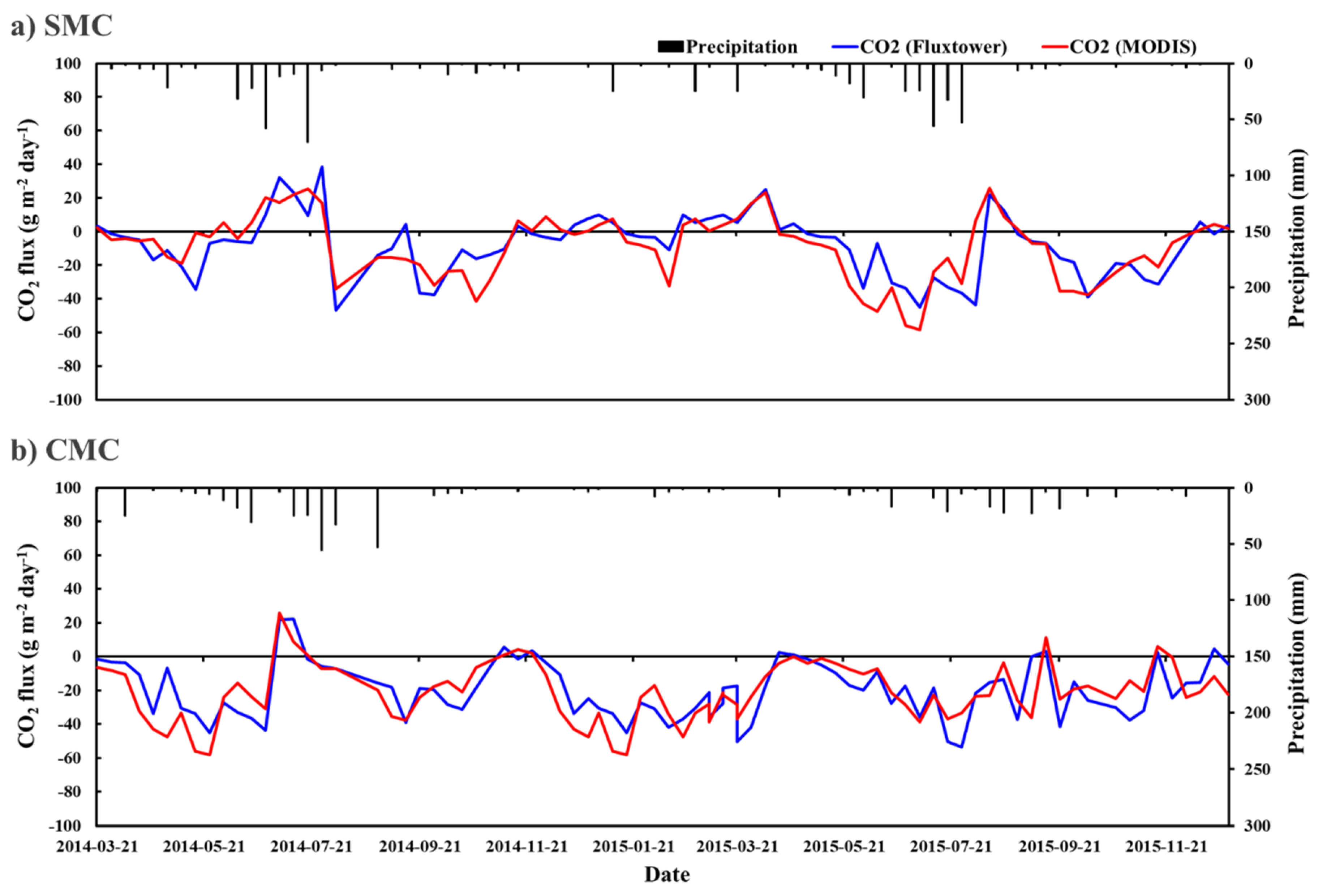
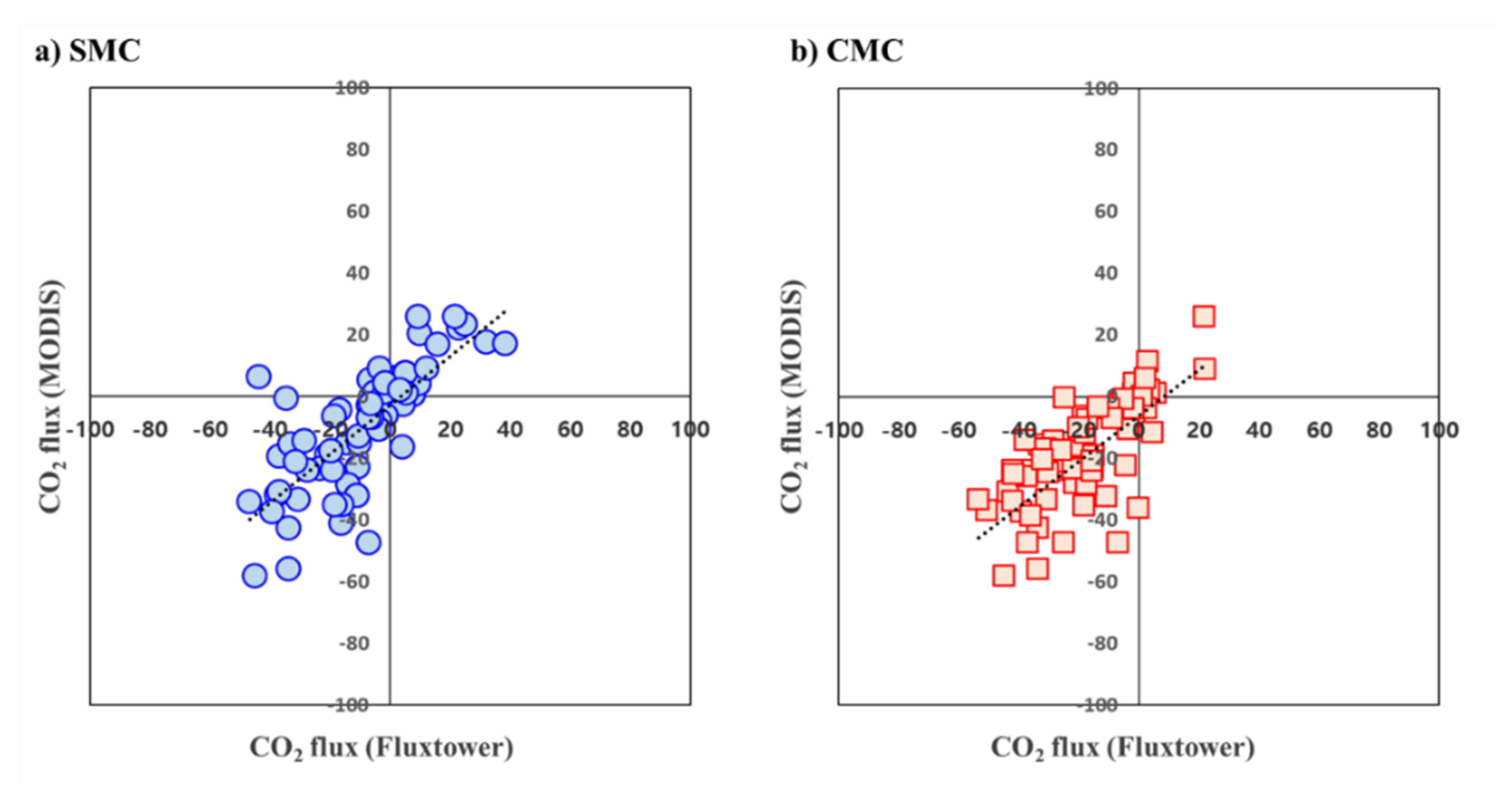
3.1.2. Temporal Variations of CO₂ Flux and Comparison with Ground Observation

According to the relationship between GPP and CO₂ presented in Section 2.3, CO₂ (hereinafter referred to as CO_{2_MODIS}) was calculated from MODIS GPP and compared with the CO₂ (hereinafter CO_{2_fluxtower}) observed in a flux tower. CO_{2_MODIS} and CO_{2_fluxtower} consist of eight-day products.

Figure 4 compares CO_{2_MODIS} and CO_{2_fluxtower} from 2014 to 2015 and compared them with the precipitation values observed in the same period. A similar tendency as the SM results in the same period can be seen in this figure after a time lag in the rainfall. As this is related to photosynthesis that occurs after SM affects vegetation activity, so that a certain duration of lag time occurs [38].

Figure 5 and

Table 4. Statistical comparison between estimated and in situ measurements of CO₂ flux.

Site	Bias (g m−2 d−1)	RMSE (g m−2 d−1)	a 1	Coefficients of Correlation
SMC	0.93	12.46	0.79	0.76 *
CMC	−1.37	12.52	0.74	0.72 *

¹ a: gradients of one on one plot. *: p-value = 0.05.

show the statistical analysis results of CO_{2_MODIS} and CO_{2_fluxtower} at two validation points. Figure 5 illustrates a one on one plot of the two results, showing a high correlation in both sites. The result of CO₂ flux is somewhat different from that of the SM were all included within the 95% confidence interval, making them statistically significant. The bias, RMSE, gradient of one on one plot, and correlation coefficients were almost similar at both SMC and CMC points, and the SMC results were better due to dense vegetation. Vegetation density is an important factor for the generation of CO₂ flux by photosynthesis in the two points. This density can be determined by the leaf area index (LAI). For SMC, LAI shows a value between 6 and 8. For CMC, LAI shows a value between 1 and 2 (Table 1). Although the difference in LAI is somewhat large, CMC is less sensitive to drought status as it is located in the rice paddy terrain where the irrigation system is built [7]. These characteristics narrowed the difference between the results of the statistical analyses of SMC and CMC [31].

3.2. Analysis of Relationship SM-VI-CO₂ under Drought Condition

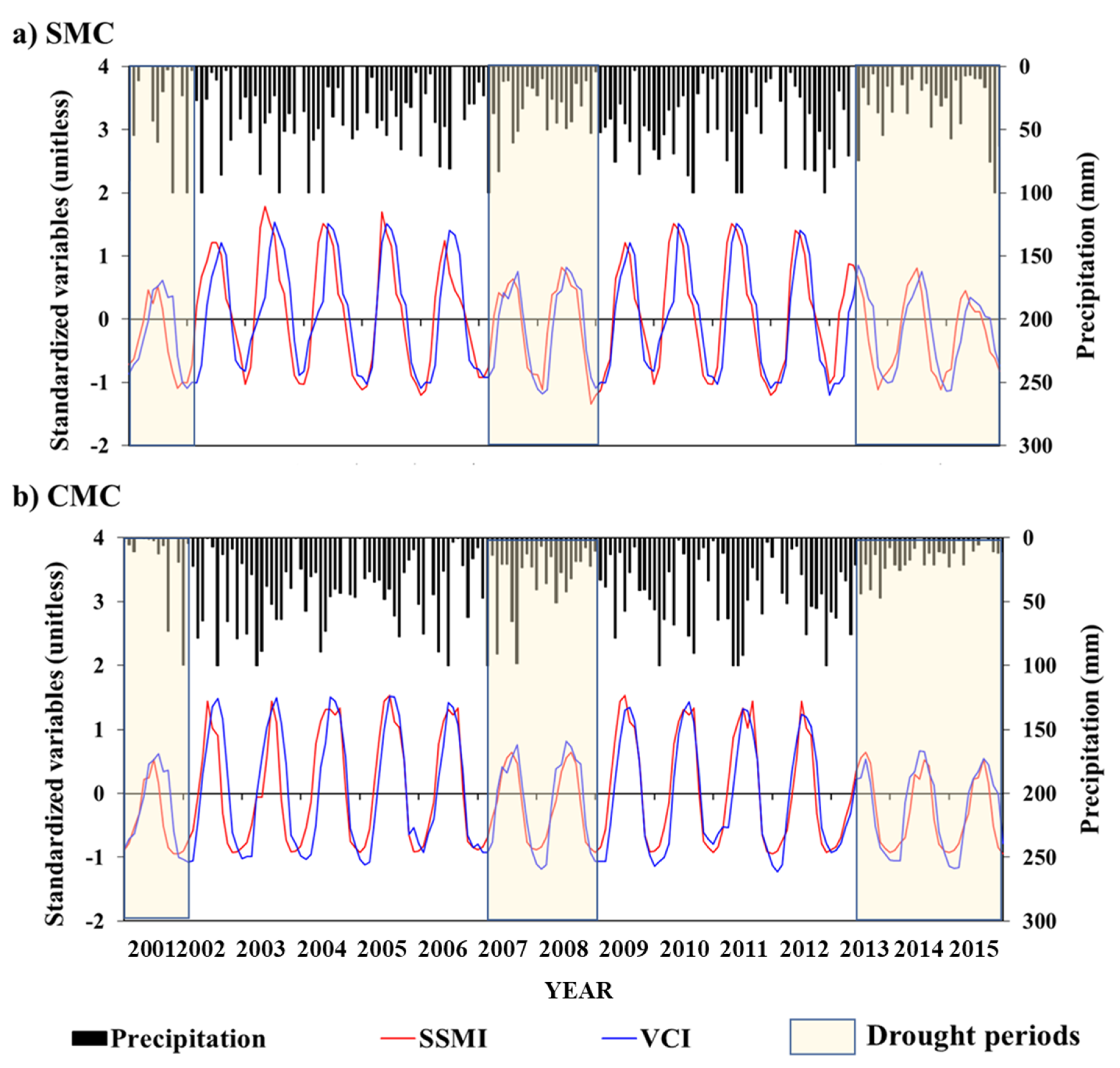
3.2.1. Selecting Drought Periods Using Agricultural Drought Indices

As per the statistical analysis of past hydrometeorological records, extreme droughts have been occurring in South Korea since the year 2000, namely in 2001, 2007 to 2009, and 2014 to 2015 [5,39,40]. Kwon et al. [39] and Kim et al. [5] analyzed droughts in Korea from 2013 to 2015. Particularly, in 2014, not only did the drought occur severely, but the recorded rainfall was less than 50% the normal. Additionally, in 2015, the region experienced only 873 mm of precipitation, which is 64% of the historical average of 1,366 mm. Variations in the monsoon climate had resulted in a dry rainy season with no precipitation [41]. Figure 6 shows the results of the temporal variation analysis of SSMI and VCI from 2001 to 2015. As with the results presented in a previous research, drought status occurred in 2001, 2007–2009, and 2014–2015. Based on the results of previous studies and Figure 6, this study chose 2014 to 2015 as the drought period.

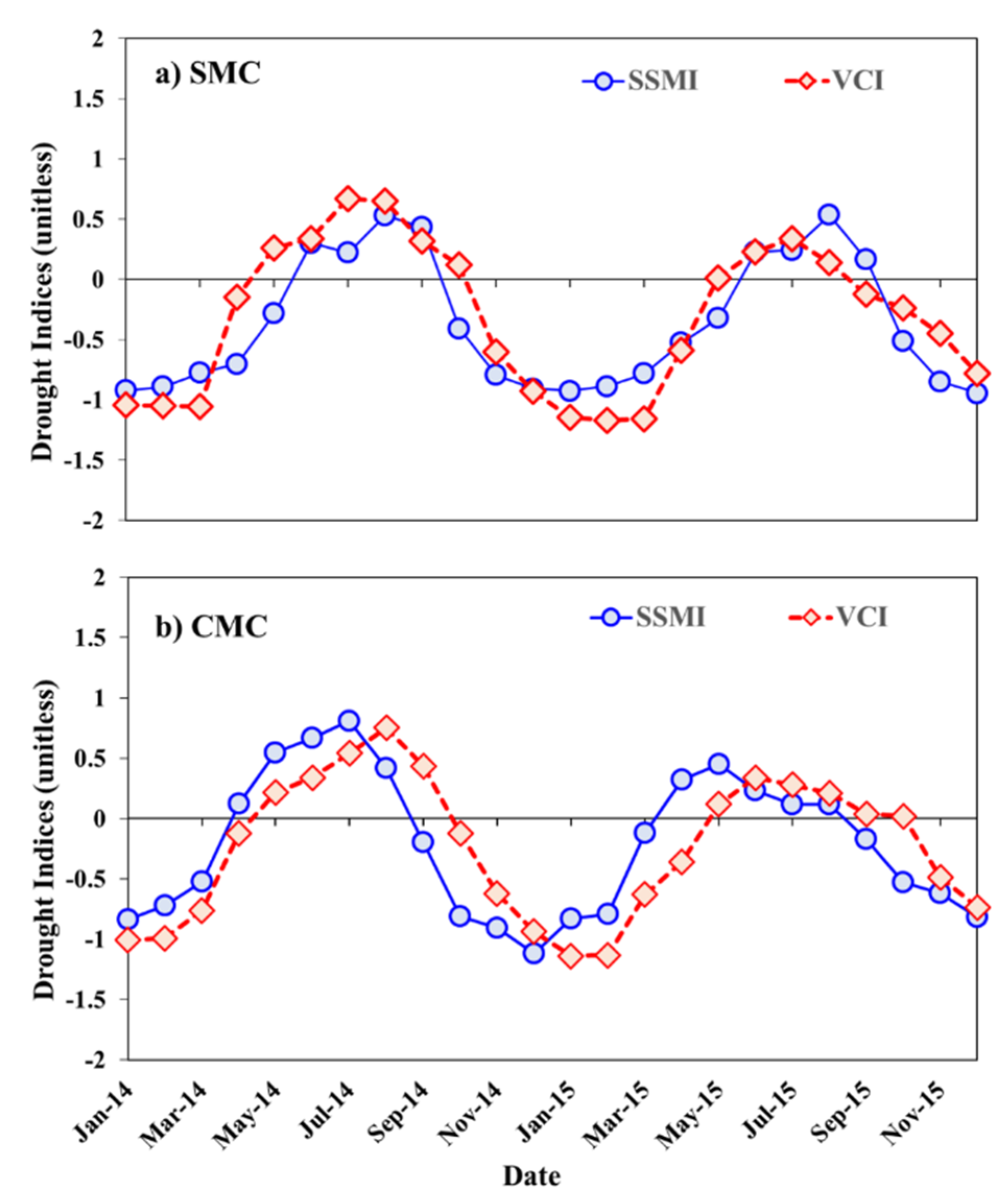
3.2.2. Drought Analysis and Validation during Drought Period

For the selected drought period, we analyzed the temporal variations of SSMI and VCI at the study sites (Figure 7). The temporal patterns of the two indices show similar tendency, with the period of the most severe drought status being October 2014 to May 2015.

Table 5. Error analysis for the study area.

(a) SMC		Soil Moisture		Sum	Drought Accuracy
		Drought	No Drought
Moderate drought ((SMfluxtower_median) = 23.14 m3 m−3)
SSMI	Drought	8	3	11	8 / 11 = 72.73%
	No drought	3	10	13
	Sum	11	13	24
VCI	Drought	7	4	11	7 / 11 = 63.64%
	No drought	5	8	13
	Sum	12	12	24
Severe drought ((SMfluxtower_lower quartile) = 8.34 m3 m−3)
SSMI	Drought	6	6	12	6 / 12 = 50.00%
	No drought	4	8	12
	Sum	10	14	24
VCI	Drought	7	5	12	7 / 12 = 58.33%
	No drought	3	9	12
	Sum	10	14	24
(b) CMC		Soil Moisture		Sum	Drought Accuracy
		Drought	No Drought
Moderate drought ((SMfluxtower_median) = 25.37 m3 m−3)
SSMI	Drought	7	2	9	7 / 9 = 77.78%
	No drought	3	12	15
	Sum	10	14	24
VCI	Drought	6	3	9	6 / 9 = 66.67%
	No drought	6	9	15
	Sum	12	12	24
Severe drought ((SMfluxtower_lower quartile) = 9.28 m3 m−3)
SSMI	Drought	5	3	8	5 / 8 = 62.50%
	No drought	8	8	16
	Sum	13	11	24
VCI	Drought	6	4	10	6 / 10 = 60.00%
	No drought	8	6	14
	Sum	14	10	24

represented the applicability of the agricultural drought indices through error analysis at two validation area. An error analysis is a formed array that consists of drought or wet conditions as compared to the category of drought by the SM_fluxtower data. The median (50%) of the standardized SM was set as the threshold for moderate drought, while the lower quantile (25%) was set as the threshold for severe drought. When the value of the standardized SM is less than the threshold, it is considered a drought condition. In the case of the samples, it is the counting of the drought indices with a value less than the threshold. The drought accuracy for SSMI and VCI at the study sites was approximately 60% to 80% (Table 5); SSMI showed relatively high accuracy for moderate drought and VCI for severe drought. SSMI is a drought index based on soil moisture that is sensitive to current soil moisture conditions and shows high accuracy under moderate drought conditions. VCI, on the other hand, is an index that detects weak vegetation activity due to lack of soil moisture, whose accuracy increases if the drought persists for a prolonged period (as the drought becomes more severe). These indices were suitable for determining the agricultural drought conditions. Each index can be used depending on how long the agricultural droughts continue.

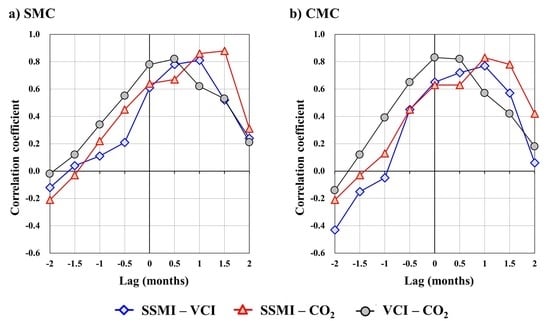
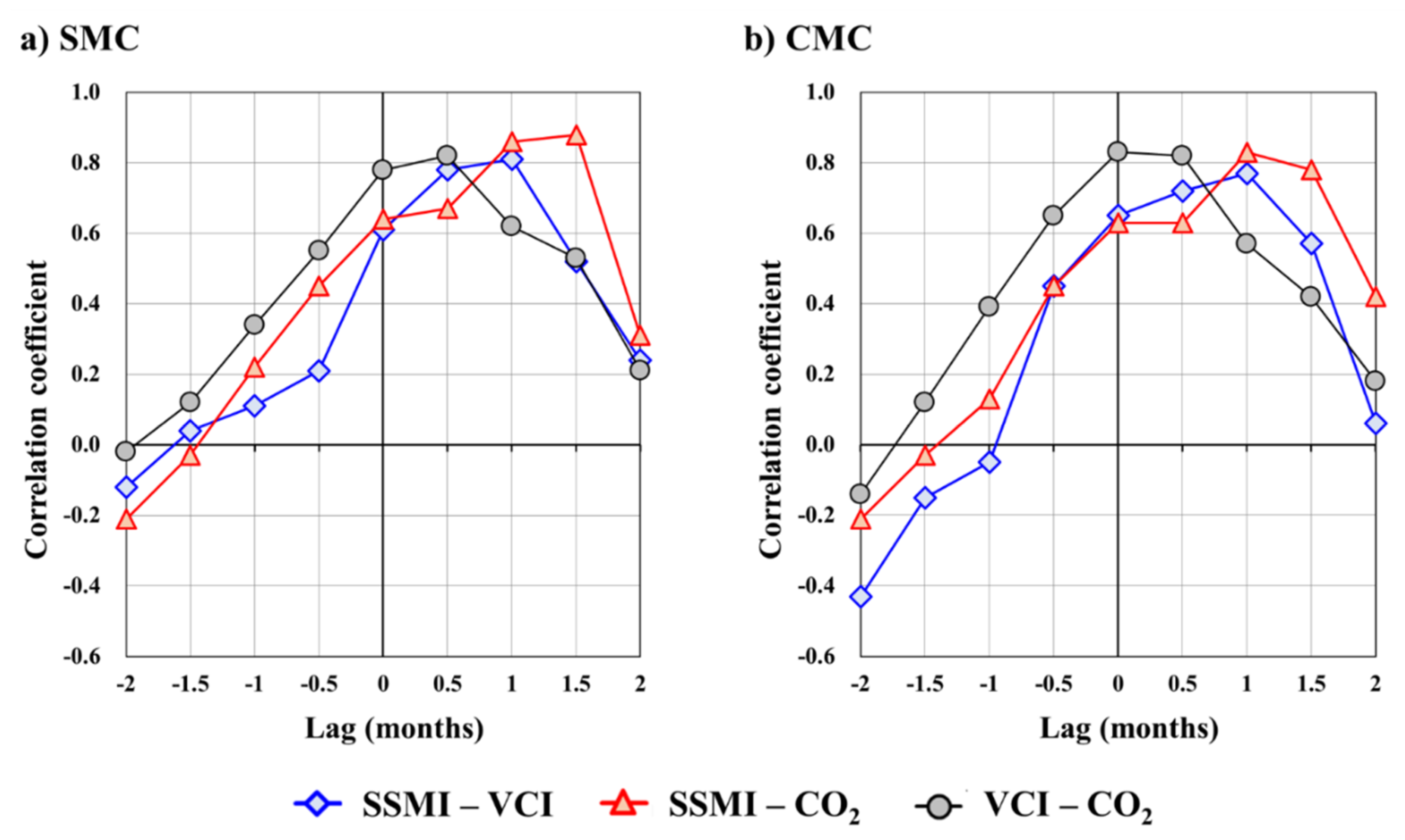
3.2.3. Relationship between SM, Vegetation and CO₂ during Drought Periods

The results mentioned above confirm the close correlation between SM, VI, and CO₂ during the drought period. Since there was a time lag between the correlations of these factors, a lag correlation was performed (Figure 8 and

Table 6. Lag correlation for study area.

(a) SMC	Lag Time (Month)
	−2.0	−1.5	−1.0	−0.5	0	0.5	1.0	1.5	2.0
SM – NDVI	−0.12	0.04	0.11	0.21	0.61	0.78 *	0.81 *	0.52	0.24
SM – CO2	−0.21	−0.03	0.22	0.45	0.64	0.67	0.86 *	0.88 *	0.31
NDVI – CO2	−0.02	0.12	0.34	0.55	0.78 *	0.82 *	0.62	0.53	0.21
(b) CMC	Lag Time (Month)
	−2.0	−1.5	−1.0	−0.5	0	0.5	1.0	1.5	2.0
SM – NDVI	−0.43	−0.15	−0.05	0.45	0.65	0.72 *	0.77 *	0.57	0.06
SM – CO2	−0.21	−0.03	0.13	0.45	0.63	0.63	0.83 *	0.78 *	0.42
NDVI – CO2	−0.14	0.12	0.39	0.65	0.83 *	0.82 *	0.57	0.42	0.18

*: p-value = 0.05.

). For homogeneous comparison of the factors, the standardized factors SM and NDVI were applied. The range of the CO₂ flux was also standardized from −1 to 1 through standardized normalization.

Figure 8 shows the result obtained from the lag correlation. Based on SM, the result showed the highest correlation for both NDVI and CO₂ after the time lag. In the case of NDVI, the highest correlation was found at a lag time of half to one month, and CO₂ showed the highest correlation at a lag time of one and a half month. When compared with the results of CO₂ correlation based on NDVI, the highest correlation was obtained at half month. Taken together, the two results reveal that the variation of SM started first followed by the variation in VI and CO₂ flux after a certain period of time.

Choi et al. [42] studied the temporal lag of precipitation, soil moisture, evapotranspiration, and vegetation index. In their paper, the lag between SM and NDVI was approximately 16 days. However, such a result is generalized as extreme weather conditions are not considered. Therefore, the results presented in this study differ from the previous ones because they were obtained as the agricultural drought condition progressed. In extreme climatic conditions such as drought, a time lag of approximately one month between SM and VI, and half month between vegetation activity and photosynthesis had occurred.

4. Conclusions

The inter-relationship between soil moisture (SM), vegetation activity, and atmospheric CO₂ concentration was analyzed using MODerate resolution imaging spectroradiometer (MODIS), an optical multispectral sensor. The SM was also estimated using MODIS. The calculated SM_MODIS was compared with the SM_fluxtower observed in a flux tower of the study area. As a result, both points showed high correlation (SMC: 0.75, CMC: 0.66). A relatively large bias was obtained in SMC due to the influence of heterogeneous land surface albedo in mixed forest areas. In the case of atmospheric CO₂ flux, MODIS gross primary productivity (GPP) product was used to leverage the flux’s relationship with respiration in the calculation. Similarly, the calculated results were compared with the CO₂ flux results of SMC and CMC to confirm their applicability. The flux values proved the relatively high applicability of the SMC result, which is due to the effect of leaf area index (LAI). This implies SMC in a dense forest area has a high value of LAI.

Lastly, the relationship between each variable was identified by comparing SM, VI, and CO₂ under the extreme drought periods of 2014 and 2015 in South Korea. As a result, the highest correlation was obtained when there was a time lag of one month between SM and vegetation and half month between vegetation and CO₂. This tendency was similar in both SMC and CMC. As such, these three variables have been proved to affect each other with time lag, and it was confirmed that the lag is longer than the normal season during the drought period. In the long term, however, changes in atmospheric CO₂ concentration may affect carbon reservoirs in the land and the subsurface. In the future, relationship studies between SM, VI, and CO₂ on the land and the subsurface during droughts should be followed by considering sources and depletions in carbon fluxes.

References

1. Heim, J.R.R. A review of twentieth-century drought indices used in the United States. Bull. Am. Meteorol. Soc. 2002, 83, 1149–1165. [Google Scholar] [CrossRef] [Green Version]
2. Mishra, A.K.; Desai, V.R. Drought forecasting using stochastic models. Stoch. Environ. Res. Risk Assess. 2005, 19, 326–339. [Google Scholar] [CrossRef]
3. Wilhite, D.A.; Svoboda, M.D.; Hayes, M.J. Understanding the complex impacts of drought: A key to enhancing drought mitigation and preparedness. Water Resour. Manag. 2007, 21, 763–774. [Google Scholar] [CrossRef] [Green Version]
4. Wu, Z.; Mao, Y.; Li, X.; Lu, G.; Lin, Q.; Xu, H. Exploring spatiotemporal relationships among meteorological, agricultural, and hydrological droughts in Southwest China. Stoch. Environ. Res. Risk Assess. 2016, 30, 1033–1044. [Google Scholar] [CrossRef]
5. Kim, J.S.; Seo, G.S.; Jang, H.W.; Lee, J.H. Correlation analysis between Korean spring drought and large-scale teleconnection patterns for drought forecast. KSCE J. Civ. Eng. 2017, 21, 458–466. [Google Scholar] [CrossRef]
6. Sivakumar, M.V.K.; Motha, R.P.; Wilhite, D.A.; Qu, J.J. Towards a compendium on national drought policy. In Proceedings of the an Expert Meeting on the Preparation of a Compendium on National Drought Policy, World Meteorological Organization, Washington, DC, USA, 14–15 July 2011; pp. 1–135. [Google Scholar]
7. Sur, C.; Park, S.-Y.; Kim, T.-W.; Lee, J.-H. Remote sensing-based agricultural drought monitoring using hydrometeorological variables. KSCE J. Civ. Eng. 2019, 23, 5244–5256. [Google Scholar] [CrossRef]
8. Kogan, F.N. Global drought watch from space. Bull. Am. Meteorol. Soc. 1997, 78, 621–636. [Google Scholar] [CrossRef]
9. Vicente-Serrano, S.M.; Begueria, S.; Lopez-Moreno, J.I. A multiscalar drought index sensitive to global warming: The standardized precipitation evapotranspiration index. J. Clim. 2010, 23, 1696–1718. [Google Scholar] [CrossRef] [Green Version]
10. Zhang, A.; Jia, G. Monitoring meteorological drought in semiarid regions using multi-sensor microwave remote sensing data. Remote Sens. Environ. 2013, 134, 12–23. [Google Scholar] [CrossRef]
11. Keshavarz, M.R.; Vazifedoust, M.; Alizadeh, A. Drought monitoring using a soil wetness deficit index (SWDI) derived from MODIS satellite data. Agric. Water Manag. 2014, 132, 37–45. [Google Scholar] [CrossRef]
12. Moorhead, J.E.; Gowda, P.H.; Singh, V.P.; Porter, D.O.; Marek, T.H.; Howell, T.A.; Stewart, B.A. Identifying and evaluating a suitable index for agricultural drought monitoring in the Texas High Plains. J. Am. Water Resour. Assoc. 2015, 51, 807–820. [Google Scholar] [CrossRef] [Green Version]
13. Liu, X.; Zhu, X.; Pan, Y.; Li, S.; Liu, Y.; Ma, Y. Agricultural drought monitoring: Progress, challenges, and prospects. J. Geogr. Sci. 2016, 26, 750–767. [Google Scholar] [CrossRef] [Green Version]
14. Sánchez, N.; González-Zamora, A.; Martínez-Fernández, J.; Piles, M.; Pablos, M. Integrated remote sensing approach to global agricultural drought monitoring. Agric. For. Meteorol. 2018, 259, 141–153. [Google Scholar] [CrossRef]
15. Peters, A.J.; Walter-Shea, E.A.; Ji, L.; Vliia, A.; Hayes, M.; Svoboda, M.D. Drought monitoring with NDVI-based standardized vegetation–index. Photogramm. Eng. Rem. Sens. 2002, 68, 71–75. [Google Scholar]
16. Bajgain, R.; Xiao, X.; Wagle, P.; Basara, J.; Zhou, Y. Sensitivity analysis of vegetation indices to drought over two tallgrass prairie sites. ISPRS J. Photogramm. 2015, 108, 151–160. [Google Scholar] [CrossRef]
17. Dong, C.; MacDonald, G.M.; Willis, K.; Gillespie, T.W.; Okin, G.S.; Williams, A.P. Vegetation responses to 2012–2016 drought in Northern and Southern California. Geophys. Res. Lett. 2019, 46, 3810–3821. [Google Scholar] [CrossRef]
18. Hu, X.; Ren, H.; Tansey, K.; Zheng, Y.; Ghent, D.; Liu, X.; Yan, L. Agricultural drought monitoring using European Space Agency Sentinel 3A land surface temperature and normalized difference vegetation index imageries. Agric. For. Meteorol. 2019, 279, 107707. [Google Scholar] [CrossRef]
19. Njoku, E.G.; Jackson, T.J.; Lakshmi, V.; Chan, T.K.; Nghiem, S.V. Soil moisture retrieval from AMSR-E. IEEE Trans. Geosci. Remote 2003, 41, 215–229. [Google Scholar] [CrossRef]
20. Cho, E.; Choi, M.; Wagner, W. An assessment of remotely sensed surface and root zone soil moisture through active and passive sensors in northeast Asia. Remote Sens. Environ. 2015, 160, 166–179. [Google Scholar] [CrossRef]
21. Anam, R.; Chishtie, F.; Ghuffar, S.; Qazi, W.; Shahid, I. Inter-comparison of SMOS and AMSR-E soil moisture products during flood years (2010–2011) over Pakistan. Eur. J. Remote Sens. 2017, 50, 442–451. [Google Scholar] [CrossRef] [Green Version]
22. Portal, G.; Jagdhuber, T.; Vall-llossera, M.; Camps, A.; Pablos, M.; Entekhabi, D.; Piles, M. Assessment of Multi-Scale SMOS and SMAP Soil Moisture Products across the Iberian Peninsula. Remote Sens. 2020, 12, 570. [Google Scholar] [CrossRef] [Green Version]
23. Deng, K.A.K.; Lamine, S.; Pavlides, A.; Petropoulos, G.P.; Bao, Y.; Srivastava, P.K.; Guan, Y. Large Scale Operational Soil Moisture Mapping from Passive MW Radiometry: SMOS product evaluation in Europe & USA. Int. J. Appl. Earth Obs. 2019, 80, 206–217. [Google Scholar] [CrossRef]
24. Verstraeten, W.W.; Veroustraete, F.; van der Sande, C.J.; Grootaers, I.; Feyen, J. Soil moisture retrieval using thermal inertia, determined with visible and thermal spaceborne data, validated for European forests. Remote Sens. Environ. 2006, 101, 299–314. [Google Scholar] [CrossRef]
25. Chang, T.-Y.; Wang, Y.-C.; Feng, C.-C.; Ziegler, A.D.; Giambelluca, T.W.; Liou, Y.-A. Estimation of root zone soil moisture using apparent thermal inertia with MODIS imagery over a tropical catchment in Northern Thailand. IEEE J. Sel. Top. Appl. 2012, 5, 752–761. [Google Scholar] [CrossRef]
26. Van doninck, J.; Peters, J.; De Baets, B.; De Clercq, E.M.; Ducheyne, E.; Verhoest, N.E.C. The potential of multitemporal Aqua and Terra MODIS apparent thermal inertia as a soil moisture indicator. Int. J. Appl. Earth Obs. Geoinf. 2011, 13, 934–941. [Google Scholar] [CrossRef]
27. Ghilain, N.; Arboleda, A.; Batelaan, O.; Ardö, J.; Trigo, I.; Barrios, J.-M.; Gellens-Meulenberghs, F. A New Retrieval Algorithm for Soil Moisture Index from Thermal Infrared Sensor On-Board Geostationary Satellites over Europe and Africa and Its Validation. Remote Sens. 2019, 11, 1968. [Google Scholar] [CrossRef] [Green Version]
28. Running, S.W.; Nemani, R.R. Relating seasonal patterns of the AVHRR vegetation index to simulated photosynthesis and transpiration of forests in different climates. Remote Sens. Environ. 1988, 24, 347–367. [Google Scholar] [CrossRef]
29. Gamon, J.A.; Field, C.B.; Goulden, M.L.; Griffin, K.L.; Hartley, A.E.; Joel, G.; Peñuelas, J.; Valentini, R. Relationships between NDVI, canopy structure, and photosynthesis in three californian vegetation types. Ecol. Appl. 1995, 5, 28–41. [Google Scholar] [CrossRef] [Green Version]
30. Muraoka, H.; Noda, H.M.; Nagai, S.; Motohka, T.; Saitoh, T.M.; Nasahara, K.N.; Saigusa, N. Spectral vegetation indices as the indicator of canopy photosynthetic productivity in a deciduous broadleaf forest. J. Plant Ecol. 2013, 6, 393–407. [Google Scholar] [CrossRef] [Green Version]
31. Sur, C.; Kang, S.; Kim, J.-S.; Choi, M. Remote sensing-based evapotranspiration algorithm: A case study of all sky conditions on a regional scale. GISci. Remote Sens. 2015, 52, 627–642. [Google Scholar] [CrossRef]
32. NASA earthdata website. Available online: https://search.earthdata.nasa.gov/search (accessed on 10 October 2019).
33. Kwon, H.; Park, S.; Kang, M.; Yoo, J.; Yuan, R.; Kim, J. Quality control and assurance of eddy covariance data at two KoFlux sites. Korean J. Agric. For. Meteorol. 2007, 9, 260–267. [Google Scholar] [CrossRef] [Green Version]
34. Amthor, J.S.; Chen, J.M.; Clein, J.S.; Frolking, S.E.; Goulden, M.L.; Grant, R.F.; Kimball, J.S.; King, A.W.; McGuire, A.D.; Nikolov, N.T.; et al. Boreal forest CO2 exchange and evapotranspiration predicted by nine ecosystem process models: Intermodal comparisons and relationships to field measurements. J. Geophys. Res. Atmos. 2001, 106, 33623–33648. [Google Scholar] [CrossRef] [Green Version]
35. Kramer, K.; Leinonen, I.; Bartelink, H.H.; Berbigier, P.; Borghetti, M.; Bernhofer, C.H.; Cienciala, E.; Dolman, A.J.; Froer, O.; Gracia, C.A.; et al. Evaluation of six process-based forest growth models using eddy-covariance measurements of CO2 and H2O fluxes at six forest sites in Europe. Glob. Chang. Biol. 2002, 8, 213–230. [Google Scholar] [CrossRef]
36. Hanson, P.J.; Amthor, J.S.; Wullschleger, S.D.; Wilson, K.B.; Grant, R.F.; Hartley, A.; Hui, D.; Hunt, E.R.; Johnson, D.W.; Kimball, J.S.; et al. Oak forest carbon and water simulations: Model intercomparisons and evaluations against independent data. Ecol. Monogr. 2004, 74, 443–489. [Google Scholar] [CrossRef] [Green Version]
37. Lloyd, J.; Taylor, J.A. On the temperature dependence of soil respiration. Funct. Ecol. 1994, 8, 315–323. [Google Scholar] [CrossRef]
38. Sur, C.; Choi, M. Evaluating ecohydrological impacts of vegetation activities on climatological perspectives using MODIS gross primary productivity and evapotranspiration products at Korean regional flux network site. Remote Sens. 2013, 5, 2534–2553. [Google Scholar] [CrossRef] [Green Version]
39. Kwon, H.-H.; Lall, U.; Kim, S.-J. The unusual 2013–2015 drought in South Korea in the context of a multicentury precipitation record: Inferences from a nonstationary, multivariate, Bayesian copula model. Geophys. Res. Lett. 2016, 43, 8534–8544. [Google Scholar] [CrossRef]
40. Park, S.Y.; Sur, C.; Kim, J.S.; Lee, J.H. Evaluation of multi-sensor satellite data for monitoring different drought impacts. Stoch. Environ. Res. Risk Assess. 2018, 32, 2551–2563. [Google Scholar] [CrossRef]
41. Lee, J.H.; Park, S.Y.; Kim, J.S.; Sur, C.; Chen, J. Extreme drought hotspot analysis for adaptation to a changing climate: Assessment of applicability to the five major river basins of the Korean Peninsula. Int. J. Climatol. 2018, 38, 4025–4032. [Google Scholar] [CrossRef]
42. Choi, M.; Mu, Q.; Kim, H.; Hwang, K.; Hur, J. Ecosystem-dynamics link to hydrologic variations for different land-cover types. Terr. Atmos. Ocean. Sci. 2017, 28, 437–462. [Google Scholar] [CrossRef] [Green Version]
Figure 1. Geographical locations of South Korea and the two flux towers ((a) Seolmacheon (SMC) and (b) Cheongmicheon (CMC) site) used in this study.
Remotesensing 12 01359 g001
Figure 2. Temporal variations of average daily soil moisture at (a) Seolmacheon (SMC) and (b) Cheongmicheon (CMC) site.
Remotesensing 12 01359 g002
Figure 3. Comparisons between observed and estimated soil moisture at (a) SMC and (b) CMC site.
Remotesensing 12 01359 g003
Figure 4. Temporal variations of average eight-day CO2 flux at at (a) SMC and (b) CMC site.
Remotesensing 12 01359 g004
Figure 5. Comparison between observed and estimated CO2 flux using 1 on 1 plot at (a) SMC and (b) CMC site.
Remotesensing 12 01359 g005
Figure 6. Temporal variations of drought indices and precipitation from 2001 to 2015 at (a) SMC and (b) CMC site.
Remotesensing 12 01359 g006
Figure 7. Temporal variations of SSMI and VCI during drought periods at (a) SMC and (b) CMC site.
Remotesensing 12 01359 g007
Figure 8. Lag correlation plot of SM, NDVI, and CO2 flux at at a) SMC and b) CMC site.
Remotesensing 12 01359 g008