Evaluation of Atmospheric Correction Algorithms for Sentinel-2-MSI and Sentinel-3-OLCI in Highly Turbid Estuarine Waters

Abstract

The present study assesses the performance of state-of-the-art atmospheric correction (AC) algorithms applied to Sentinel-2-MultiSpectral Instrument (S2-MSI) and Sentinel-3-Ocean and Land Color Instrument (S3-OLCI) data recorded over moderately to highly turbid estuarine waters, considering the Gironde Estuary (SW France) as a test site. Three spectral bands of water-leaving reflectance ($Rhow$) are considered: green (560 nm), red (655 or 665 nm) and near infrared (NIR) (865 nm), required to retrieve the suspended particulate matter (SPM) concentrations in clear to highly turbid waters (SPM ranging from 1 to 2000 mg/L). A previous study satisfactorily validated Acolite short wave infrared (SWIR) AC algorithm for Landsat-8-Operational Land Imager (L8-OLI) in turbid estuarine waters. The latest version of Acolite Dark Spectrum Fitting (DSF) is tested here and shows very good agreement with Acolite SWIR for OLI data. L8-OLI satellite data corrected for atmospheric effects using Acolite DSF are then used as a reference to assess the validity of atmospheric corrections applied to other satellite data recorded over the same test site with a minimum time difference. Acolite DSF and iCOR (image correction for atmospheric effects) are identified as the best performing AC algorithms among the tested AC algorithms (Acolite DSF, iCOR, Polymer and C2RCC (case 2 regional coast color)) for S2-MSI. Then, the validity of six different AC algorithms (OLCI Baseline Atmospheric Correction (BAC), iCOR, Polymer, Baseline residual (BLR), C2RCC-V1 and C2RCC-V2) applied to OLCI satellite data is assessed based on comparisons with OLI and/or MSI Acolite DSF products recorded on a same day with a minimum time lag. Results show that all the AC algorithms tend to underestimate $Rhow$ in green, red and NIR bands except iCOR in green and red bands. The iCOR provides minimum differences in green (slope = 1.0 ± 0.15, BIAS = 1.9 ± 4.5% and mean absolute percentage error (MAPE) = 12 ± 5%) and red (slope = 1.0 ± 0.17, BIAS = −9.8 ± 9% and MAPE = 28 ± 20%) bands with Acolite DSF products from OLI and MSI data. For the NIR band, BAC provides minimum differences (slope = 0.7 ± 0.13, BIAS = −33 ± 17% and MAPE = 55 ± 20%) with Acolite DSF products from OLI and MSI data. These results based on comparisons between almost simultaneous satellite products are supported by match-ups between satellite-derived and field-measured SPM concentrations provided by automated turbidity stations. Further validation of satellite products based on rigorous match-ups with in-situ $Rhow$ measurements is still required in highly turbid waters.

1. Introduction

Once corrected for atmospheric effects, ocean color satellite data can be used to retrieve and map suspended particulate matter (SPM) concentrations ranging from 1 to 2000 mg/L in coastal and estuarine waters [1]. Atmospheric correction (AC) is a crucial step in the processing of ocean color remote sensing data to derive water biogeochemical parameters [2,3]. Over the open ocean, around 90% of the radiance received by satellite sensors results from the atmospheric contribution. In coastal waters, these contributions can be higher than 90% especially in the blue and green bands but are usually much lower in the red and near infrared (NIR) bands in the case of highly turbid waters associated with a higher reflectance signal [4]. In the ocean–atmosphere system, the radiance detected at the top of the atmosphere ($L_t\left(\lambda \right)$) can be portioned linearly into various distinct physical contributions [5,6]:

$$L_t\left(\lambda \right)=L_r\left(\lambda \right)+L_a\left(\lambda \right)+L_{aR}\left(\lambda \right)+L_g\left(\lambda \right)\times T\left(\lambda \right)+L_{wc}\left(\lambda \right)\times t\left(\lambda \right)+L_w\left(\lambda \right)\times t\left(\lambda \right)$$

(1)

where $L_t\left(\lambda \right)$ is the total radiance measured by the sensor (radiance is the spectral flux that reaches the instrument per unit area per unit of solid angle and per unit wavelength with unit $W{m}^{-2}s{r}^{-1}n{m}^{-1}$), $\lambda$ is the wavelength, $L_r\left(\lambda \right)$ is the radiance due to Rayleigh scattering by air molecules, $L_a\left(\lambda \right)$ is the radiance due to aerosols (includes light scattering/absorption by aerosols), $L_{aR}$ is the radiance due to aerosols-molecules scattering, $L_g$ is the Sun-glint radiance, $L_{wc}$ is the surface white caps radiance and $L_w$ is the water-leaving radiance. T and t are the atmospheric direct and diffuse transmittances. The normalized water-leaving radiance ($L_{WN}$) is the $L_w$ that would occur if the Earth was at one astronomical unit (AU) from the Sun, the Sun was at the zenith and the atmosphere was non attenuating [7]. $L_{WN}$ signal is computed by the following equation [8]:

$$L_{WN}({\theta }_v,\varphi )\equiv {\left(\frac{R}{R_o}\right)}^2\frac{L_w({\theta }_s,{\theta }_v,\varphi )}{cos\left({\theta }_s\right)t\left({\theta }_s\right)}$$

(2)

where R is the Earth–Sun distance at the time of measurement and $R_o$ is the mean Earth–Sun distance, ${\theta }_s$ is the Sun zenith angle, ${\theta }_v$ is the satellite viewing direction and $\varphi$ is the azimuthal angle measured relative to the Sun’s azimuthal direction. The factors ${\left(\frac{R}{R_o}\right)}^2$, $cos\left({\theta }_s\right)$ and $t\left({\theta }_s\right)$ largely remove the effects of Earth–Sun distance, solar zenith angle and atmospheric attenuation on measured $L_w$. $L_{WN}$ still depends on particular viewing direction and the sky angular radiance distribution at the time of observation. The non-dimensional water-leaving reflectance is derived by the following equation [9,10].

$$Rhow\equiv \left(\frac{\pi }{F_o}\right)L_{WN}({\theta }_v,\varphi )=\pi \times R_{rs}$$

(3)

where $\pi$ has units of steradian, $F_o$ is the extraterrestrial solar irradiance with unit $W{m}^{-2}n{m}^{-1}$ measured at mean Earth–Sun distance and $R_{rs}$ is the remote sensing reflectance with unit $s{r}^{-1}$.

Standard AC algorithms perform well in open ocean waters. These standard AC algorithms estimate the aerosol radiance by assuming a negligible water-leaving radiance (black pixel assumption) in NIR bands due to strong light absorption by pure water [9,11,12]. NIR bands are then used to estimate the atmospheric contribution and then extrapolate it to the visible bands. When dealing with coastal and inland turbid waters, these algorithms usually fail to retrieve $Rhow$ due to enhanced light backscattering by suspended particles, so that the water-leaving signal is no longer negligible in NIR bands. It is therefore necessary to separate the aerosol and marine contributions from the top of the atmosphere. As the NIR based black pixel assumption is no longer valid in turbid waters [11,13,14,15], short wave infrared (SWIR) based AC algorithms can be a solution [12,16]. A NIR-SWIR combined method has been proposed [17,18,19] for MODIS (MODerate resolution Imaging Spectroradiometer). This approach derives the $Rhow$ using the standard algorithm (NIR) for non-turbid waters and a SWIR algorithm for turbid waters. Other AC methods have been developed for turbid waters: the bright pixel atmospheric correction (BPAC) [20], AC for turbid and inland waters [13], the semi empirical radiative transfer (SERT) model [21], a neural network (NN) model (C2RCC) [22], spectral matching method (Polymer) [23], the NIR-SWIR approach [18], the SWIR exponential [24,25] and SWIR Dark Spectrum Fitting (DSF) [26,27].

Many studies did assess the performance of existing AC algorithms in moderately turbid waters for different satellite sensors such as SeaWiFS (Sea-Viewing Wide Field-of-View Sensor) [28], MODIS-Aqua [29], GOCI (Geostationary Ocean Color Imager) [30], L8-OLI [31,32,33,34,35,36], S2-MSI [36,37,38,39,40,41] and S3-OLCI [42,43]. None of these studies considered the case of highly turbid waters for S3-OLCI. The objective of the present study is to identify the best performing AC algorithms for S2-MSI and S3-OLCI in the scope of deriving SPM concentrations in highly turbid waters.

The paper is organized as follows: in the first section, we present the study area, data and methods adopted for the intercomparison exercise between different ocean color sensors. The next section primarily investigates the performance of various AC algorithms to retrieve $Rhow$ from S2-MSI data and identifies the best performing AC algorithm for S2-MSI. Next considers the performance of available AC algorithms to retrieve $Rhow$ from S3-OLCI and identifies the best performing AC algorithm/s. Eventually, the comparison between $Rhow$ derived from various AC processors for OLCI satellite data and in-situ data is presented followed by the validation of satellite-derived SPM (S2-MSI/L8OLI and S3-OLCI) using in-situ turbidity measurements from autonomous stations.

2. Materials and Methods

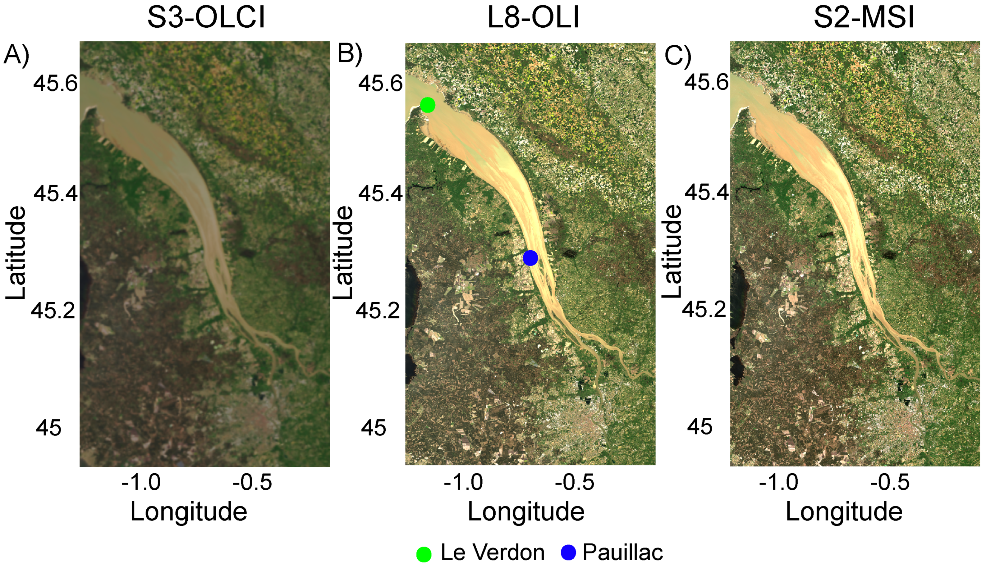
The validation of AC algorithms is usually based on match-ups between satellite and field data [44,45]. Due to the unavailability of a large number of in-situ data in highly turbid waters, another method is used in the present study based on match-ups between already validated satellite products and satellite data corrected for atmospheric effects using different AC algorithms. Such match-ups are expected to provide pixel-by-pixel comparisons over wide areas covering a wide range of water turbidity. Here the already validated L8-OLI products derived using the Acolite SWIR AC algorithm in the moderately to highly turbid Gironde estuarine waters [1] are used as reference to assess the performance of different AC algorithms applied to S2-MSI and S3-OLCI satellite data. For that purpose, a selection of cloud-free images of S3-OLCI recorded over the Gironde Estuary during the year 2018 are considered, including match-ups with S2-MSI and/or L8-OLI satellite data.

2.1. Study Area

The Gironde Estuary is a highly turbid semi-diurnal macro tidal estuary with a tidal amplitude of 2–5.5 m [46] located in the southwest coast of France and connected to the Atlantic Ocean (Figure 1). The Garonne (watershed area 57,000 km${}^2$) and Dordogne (watershed area 24,000 km${}^2$) are the two rivers confluence into the Gironde Estuary (surface area 635 km${}^2$). The high tidal range and prominent length promote the formation of a turbidity maximum zone (TMZ) [47] with surface SPM concentrations ranging from 100 to 10,000 mg/L [48]. The SPM is mainly suspended sediments [1,49,50,51,52,53,54,55,56] and SPM concentrations are well correlated with the water turbidity independently of tidal and seasonal conditions [1,53,55,57]. This study area is equipped with autonomous monitoring stations and has been already used as a test site to calibrate and validate ocean color satellite products for SPM retrieval and mapping [49,51,52,53], based on field data-sets including hyperspectral $Rhow$, SPM concentrations and turbidity measurements [58].

2.2. Data

The data-set is composed of both field and satellite data. Field data include simultaneous measurements of surface SPM concentrations with above-water hyperspectral radiometric measurements (from field campaigns) and continuous automated measurements of water turbidity in two-optically contrasted locations along the estuary. The satellite data used in this study are the cloud-free images of L8-OLI, S2-MSI and S3-OLCI recorded over the Gironde Estuary during the year 2018.

2.2.1. In-Situ Data

In-situ data are the measurements carried out during a field campaign in 2018 and data recorded by two automated turbidity stations. A total of 50 field stations were sampled in the Gironde Estuary from 17 to 20 September 2018 with SPM, turbidity and radiometric measurements carried out for a wide range of SPM concentrations (5 to 500 mg/L), representative of moderately to highly turbid waters.

Radiometric Measurements

Three TriOS RAMSES hyperspectral (350–950 nm with a sampling interval of 3.3 nm) radiometers were used to measure the above-water downwelling irradiance ($E_d(0+,\lambda )$), upwelling radiance ($L_{sea}\left(\lambda \right)$ and the downwelling sky radiance ($L_{sky}\left(\lambda \right)$) in two optically-contrasted estuarine stations. The irradiance sensor was mounted vertically upwards, the sky and seaward pointing sensors were mounted at 40${}^{\circ }$ and 140${}^{\circ }$ from the zenith and the radiance sensors were pointed at a relative azimuth angle of 135${}^{\circ }$ away from the Sun [59,60]. The measurements for each station were performed for 10 min duration with a simultaneous sampling period of 10 s. $Rhow$ was computed using the following equation [59]:

$$Rhow\left(\lambda \right)=\pi \times \frac{[L_{sea}\left(\lambda \right)-L_{sky}\left(\lambda \right)\times {\rho }_{sky}]}{E_d(0+,\lambda )}$$

(4)

where ${\rho }_{sky}$, the air–water interface reflection coefficient for radiance, was fixed to 0.0256 [56]. The resulting $Rhow$ spectra and the spectral bands (green, red and NIR) considered in the present study are highlighted in Figure 2.

Automated Turbidity Stations

The Gironde Estuary is monitored through an automated network called MArel Gironde ESTuary (MAGEST) [61] including six stations. Two stations are located inside the estuary (Pauillac and Le Verdon) and are considered here while the others are located along the Garonne and Dordogne rivers. Pauillac is in the central part of the estuary, 52 km upstream from the mouth. Le Verdon is located at the mouth of the estuary (Figure 1). Continuous measurements of water turbidity, salinity and temperature are recorded every 20 min one meter below the surface. The turbidity sensor (Endress and Hauser, CUS31-W2A) is able to record values between 0 and 10,000 Nephelometric Turbidity Unit (NTU) with an accuracy of 10%. The sensor saturates when turbidity values are higher than 10,000 NTU, this limit corresponds to SPM concentration of 6000 mg/L [62].

2.2.2. Satellite Data

The OLCI data (Level1 and Level2) were downloaded from Copernicus Online Data Access (CODA) (https://coda.eumetsat.int) provided by EUMETSAT (European Organization for the Exploitation of Meteorological Satellites); the OLI data (Level1) were accessed from earth explorer (https://earthexplorer.usgs.gov/) provided by USGS (United States Geological Survey); MSI data (Level-1C) were accessed from Copernicus Open Access Hub (https://scihub.copernicus.eu) provided by ESA (European Space Agency) Copernicus. There are 24 totally cloud-free OLCI images recorded over the Gironde Estuary in 2018. Six match-ups with MSI data and four match-ups with OLI satellite data were identified out of these 24 OLCI images, which are representative of seasonal and tidal conditions (tidal range 2.5–5.2 m) prevailing in the Gironde Estuary (

Table 1. Date (dd/mm/yyyy) and time (UTC) of cloud-free satellite observations selected over the year 2018 and corresponding hydro-dynamical conditions prevailing in the estuary at the time of satellite overpass, LW, HW, TR, SZA, Pau-AOT865 and Ver-AOT865 respectively stand for low-water, high-water, tidal range, sun zenith angle, aerosol optical thickness at 865 nm from Pauillac station and aerosol optical thickness at 865 nm from Le Verdon station.

Date	Tide	Tide	TR (m)	SZA (${}^{\circ }$)	Pau-AOT865	Ver-AOT865	OLCI	MSI	OLI
25/02/2018	06:19 LW	12:48 HW	3.18	61.19	0.22 ± 0.19	0.23 ± 0.19	10:11
16/04/2018	04:55 HW	11:34 LW	5.02	42.09	NaN	0.30 ± 0.20	10:15
19/04/2018	06:47 HW	13:29 LW	4.78	38.65	0.61 ± 0.10	0.26 ± 0.10	10:37	11:01	10:47
20/04/2018	07:31 HW	14:08 LW	4.41	41.21	0.38 ± 0.15	0.26 ± 0.11	10:11
04/05/2018	07:14 HW	13:41 LW	3.90	32.96	0.43 ± 0.07	0.56 ± 0.13	10:48	11:02
05/05/2018	07:49 HW	14:13 LW	3.40	35.50	0.65 ± 0.18	0.38 ± 0.11	10:22		10:46
20/05/2018	08:24 HW	14:49 LW	3.99	30.95	0.39 ± 0.21	0.25 ± 0.14	10:33
20/06/2018	10:17 HW	16:35 LW	3.62	29.17	0.23 ± 0.17	0.21 ± 0.19	10:30
25/06/2018	09:15 LW	15:22 HW	3.97	33.61	0.31 ± 0.19	0.13 ± 0.12	10:00
28/06/2018	04:57 HW	11:18 LW	4.10	30.54	0.40 ± 0.22	0.17 ± 0.16	10:22	11:06
09/07/2018	07:26 LW	13:40 HW	3.58	29.59	0.32 ± 0.14	0.21 ± 0.06	10:37
10/07/2018	08:30 LW	14:35 HW	4.08	33.26	0.38 ± 0.17	0.23 ± 0.06	10:11
25/07/2018	09:37 LW	15:46 HW	3.80	33.96	0.53 ± 0.21	0.34 ± 0.14	10:22
02/08/2018	07:55 HW	14:23 LW	3.84	36.48	0.26 ± 0.18	0.10 ± 0.04	10:15	10:59
05/08/2018	04:25 LW	10:37 HW	3.08	34.32	0.18 ± 0.14	0.22 ± 0.13	10:37
06/08/2018	05:33 LW	12:01 HW	3.05	37.81	0.23 ± 0.15	0.25 ± 0.10	10:11
18/08/2018	09:54 HW	16:22 LW	3.23	42.03	0.29 ± 0.24	0.19 ± 0.19	10:00
22/08/2018	08:21 LW	14:45 HW	3.09	43.50	0.23 ± 0.17	0.26 ± 0.19	09:57	11:04
01/09/2018	08:06 HW	14:39 LW	3.89	41.52	0.08 ± 0.14	0.09 ± 0.08	10:37	10:59	10:53
02/09/2018	08:52 HW	15:24 LW	3.50	44.56	0.16 ± 0.20	0.44 ± 0.26	10:11
12/09/2018	06:25 HW	13:02 LW	5.17	43.82	0.27 ± 0.19	0.21 ± 0.19	10:52
17/09/2018	10:09 HW	16:42 LW	2.46	47.96	0.16 ± 0.13	0.23 ± 0.14	10:22		10:53
20/09/2018	07:49 LW	14:17 HW	2.74	47.08	0.23 ± 0.26	0.56 ± 0.29	10:45
24/09/2018	04:18 HW	10:43 LW	4.40	48.74	0.24 ± 0.19	0.27 ± 0.23	10:41

). The spatial resolution of each sensor is different: 30 m for OLI, 10, 20 and 60 m for MSI and 300 m for OLCI. For pixel-by-pixel intercomparison between satellite products, a spatial binning of 300 m resolution using the nearest neighbour method was implemented using the Level3-binning of Sentinel Application Platform (SNAP). For the match-ups between satellite and in-situ data, the mean satellite-derived $Rhow$ values in the 5 × 5 pixels box centered at each in-situ station were considered.

2.3. Methods

2.3.1. Bandwidth Correction

L8-OLI high spatial resolution (30 m) data are recorded at 9 spectral bands ranging from the visible to the SWIR spectral regions. The S2-MSI also performs measurements in 13 spectral bands ranging from visible to SWIR (443–2202 nm) at three spatial resolutions (10, 20 and 60 m). S3-OLCI simultaneously performs measurements in 21 spectral bands ranging from the visible to the NIR (400–1020 nm) spectral regions with a spatial resolution of 300 m. The bandwidths of the corresponding green (560), red (665 or 655) and NIR (865) spectral bands are significantly different for these three sensors. For OLI the bandwidths for green, red and NIR are 57, 37 and 28 nm, respectively. For MSI the bandwidths for green, red and NIR are 46, 39 and 33 nm, respectively. These bandwidths are wide compared to the corresponding OLCI bands (10, 10 and 20 nm, respectively) (Figure 3).

Taking into account the spectral response functions (SRF) of each sensor, correspondence functions were established between the $Rhow$ values of OLI, MSI and OLCI in the three spectral bands (green, red and NIR) using the in-situ measured hyperspectral $Rhow$ values. The resulting correspondence functions closely follow 1:1 relationships (Figure 4), which means band-to-band $Rhow$ comparisons can be made between these different sensors even without considering the correspondence functions.

2.3.2. Selected Atmospheric Correction Algorithms

The list of the AC algorithms considered for each sensor is shown in

Table 2. List of atmospheric correction algorithms tested for each sensor.

L8-OLI	S2-MSI	S3-OLCI
Acolite DSF/SWIR	Acolite DSF	BAC
iCOR (NoSIMEC and SIMEC)	iCOR (NoSIMEC and SIMEC)	iCOR (NoSIMEC and SIMEC)
	Polymer	Polymer
	C2RCC	BLR
		C2RCC-V1
		C2RCC-V2

. Almost all available AC algorithms specially designed for coastal and turbid waters were considered. Due to the unavailability of codes, some AC algorithms were omitted from the present study [21,42,63,64].

AC Algorithms Considered for S2-MSI

Acolite DSF: The Acolite processor is an AC algorithm developed by the Royal Belgian Institute of Natural Sciences [25]. It applies by default the Dark Spectrum Fitting (DSF) approach [26,27]. This AC scheme is exclusively image-based and hence does not need external inputs such as aerosol optical thickness (measured or estimated). This scheme assumes that the atmosphere is homogeneous over a scene or sub-scene. This hypothesis allows the atmospheric path reflectance to be predicted from multiple dark targets in the scene or sub-scene. These targets are selected accordingly to the lowest observed top of atmosphere reflectance values in all the bands. The L8-OLI and S2-MSI sensors have SWIR bands (at 1.6 and 2.2 $\mathsf{\mu }$m), where $Rhow$ can be assumed negligible even for extremely turbid waters [16,24]. Acolite can also be configured into the SWIR approach [24,25] by changing the aerosol correction to exponential in the settings file. This AC algorithm is designed for clear to turbid waters and can be adapted to most satellite sensors, but it requires SWIR bands to work over turbid waters.

iCOR for MSI/OLI: Image correction for atmospheric effects (iCOR) is an image-based AC tool which runs through multiple processing steps [65]. First, the workflow identifies the land and water pixels based on a band threshold. Secondly, land pixels are used to estimate the aerosol optical thickness (AOT). The raw top of the atmosphere (TOA) image is subdivided into tiles of about 15 × 15 km, small enough to assume atmospheric homogeneity and large enough to include sufficient spectral variability. A maximum AOT threshold is defined for each sub-tile using the dark dense vegetation (DDV) approach. These maximum AOT values are further refined using the spectral variation within the sub-tile, through a multi-parameter end-member inversion technique using selected end-members (ranging from bare soil to highly vegetated pixels). The AOT values retrieved over land pixels are extrapolated over water. In the next step, an adjacency correction can optionally be applied using the SIMilarity Environmental Correction (SIMEC) approach [66]. Finally the radiative transfer equation will be solved using MODerate resolution atmospheric TRANsmission (MODTRAN-5) Look-Up-Tables (LUT). For water pixels, an additional correction for Fresnel reflectance is applied.

C2RCC: The “Case 2 Regional processor” is a Neural Network (NN) based AC algorithm originally proposed by [67] with a large set of radiative transfer simulations inverted by NN. This method has been revised with an additional set of NN computations specially trained to cover wide ranges of water scattering and absorption coefficients, called as Case 2 Regional Coast Color (C2RCC) [22]. As we did not observe a significant improvement from C2RCC apart from large numbers of flagged pixels [40], the C2X alternate net was not incorporated in the present study. The C2RCC processor used for MSI is called C2RCC hereafter.

Polymer: The Polynomial based algorithm applied to MERIS (Polymer) is an AC algorithm specially designed for waters with and without sun-glint contamination [23]. Polymer works on the principle of the spectral matching method. This method depends upon a polynomial function to model the spectral reflectance of the atmosphere and Sun-glint with the help of a water reflectance model available for visible and also extended to NIR (700 to 900 nm) bands using the similarity spectrum for turbid waters [68].

AC Algorithms Tested for S3-OLCI

OLCI Baseline AC (BAC): The OLCI Baseline AC algorithm (BAC) is a combination of NIR based black pixel assumption accommodated with the multiple scattering of air molecules and aerosols [69,70] together with the BPAC [20]. The BPAC corrects the contribution of sediments on $Rhow$. It consists in decoupling the oceanic and atmospheric components in the NIR bands, in order to apply the standard atmospheric correction scheme. $Rhow$ in NIR bands is computed using an iterative approach. The BPAC version used in the present OLCI data is that inherited from last MERIS reprocessing [71]. The BAC algorithm also considers the correction of the blue absorbing aerosols [72].

iCOR for OLCI: Two adaptations were added in the iCOR workflow for the processing of OLCI images, compared to MSI/OLI. First, an additional limitation has been defined in the AOT extrapolation step from land to water: the resulting $Rhow$ (without adjacency correction) in band Oa11 (709 nm) or Oa18 (885 nm) is not allowed to be negative. When this happens, the AOT value will be adapted accordingly. Secondly, an additional glint and haze correction has been included: the water leaving reflectance at Oa21 (1020 nm) is subtracted from the retrieved $Rhow$. This additional correction is only performed on unmixed (land/water) pixels and in absence of remaining adjacency effects. When $Rhow$ at Oa21 (1020 nm) exceeds $Rhow$ at Oa17 (865 nm), e.g., due to calibration issues, this atter band will be used for subtraction instead of Oa21.

Polymer: The description of the Polymer AC algorithm is available in the previous paragraph AC algorithms tested for S2-MSI.

Baseline residual (BLR): Using the single SWIR band (1016 nm) of OLCI, a new AC algorithm specially designed for highly turbid waters was proposed by [73]. The algorithm depends on a spectral magnitude which is substantially independent of the atmospheric conditions called the BLR (Baseline residual), which is the Rayleigh-corrected reflectance of the middle band of specially selected triple bands after baseline subtraction. It uses three consecutive triplets of OLCI bands (620–709–779 nm, 709–779–865 nm and 779–865–1016 nm) to calculate $Rhow$ and hence the aerosol reflectance at these wavelengths.

C2RCC-V1 and C2RCC-V2: The C2RCC processor has been developed for different satellite sensors [22,67]. In this study, C2RCC processors for OLCI are named C2RCC-V1 (available in SNAP 6.0) and C2RCC-V2 (available in SNAP 7.0). C2RCC-V1 is the basic AC algorithm with C2RCC net, while C2RCC-V2 is a more advanced NN (alternative NN) trained for several water types based on European Space Agency (ESA) case2extreme findings (personal communication with C. Lebreton). C2RCC-V2 provides better coverage of highly backscattering waters (rivers, estuaries and lakes). The combination of noise training data set and NN architecture optimized in the C2RCC-V2 reduce the noise compared to C2RCC-V1.

2.3.3. SPM Extraction

The in-situ SPM is derived from the turbidity values (NTU) measured from the two automated stations. The turbidity were converted into SPM concentrations (mg/L) using [1]:

$$SPM=0.88\times Turbidity$$

(5)

The two consecutive turbidity measurements just before and after each satellite overpass were used to compute the time-averaged turbidity mean value matching the satellite-derived product.

Satellite-derived SPM concentrations are obtained by applying to satellite-derived $Rhow$ values the SPM model developed by [1]. This model retrieves SPM concentrations within the wide range (1–2000 mg/L) encountered in moderately to extremely turbid estuarine waters by switching from green to red then NIR bands. The switching criteria are based upon the $Rhow$ values derived from the saturation points of the most sensitive bands (green, red and NIR). The switching limits were selected by band comparison between in-situ $Rhow$ values: $Rhow$ (green) versus $Rhow$ (red) and $Rhow$ (red) versus $Rhow$ (NIR) (see details in [1] ). In the present study, the switching SPM algorithm is applied to $Rhow$ values derived from OLCI satellite data applying the BAC algorithm and from MSI/OLI data applying the Acolite DSF AC algorithm.

2.3.4. Statistical Analyses

For this pixel-by-pixel multi-sensor intercomparison exercise between $Rhow$ values derived using different AC algorithms, a spatial binning was performed using the nearest neighbour method for all the 3 sensors into regular grids with the same spatial resolution (300 m). At first step, the spatial distributions of green, red and NIR $Rhow$ values along the estuary were compared based on satellite maps (qualitative comparisons). Then quantitative comparisons were performed based on scatter-plots between S3-OLCI $Rhow$ values (y-axis) and S2-MSI or L8-OLI $Rhow$ values used as references (x-axis). The quantitative comparisons were then based on five different statistical indicators: the slope of the linear fit (slope) and corresponding coefficient of determination ($r^2$), the normalized root mean square error (NRMSE %), the Bias (BIAS %) and mean absolute percentage error (MAPE %). The AC algorithm associated to the maximum number of favorable statistical indicators was considered as the best performing AC algorithm. The equations of NRMSE, BIAS and MAPE are shown below:

$$RMSE=\sqrt{\frac{{\sum }_{i=1}^n{(Rho{w}_{A{C}_i}\left(\lambda \right)-Rho{w}_{RE{F}_i}\left(\lambda \right))}^2}{n}}$$

(6)

$$NRMSE(\%)=\left[\frac{RMSE}{Max\left(Rho{w}_{REF}\left(\lambda \right)\right)-Min\left(Rho{w}_{REF}\left(\lambda \right)\right)}\right]\times 100$$

(7)

$$BIAS(\%)=\frac{{\sum }_{i=1}^n\left[Rho{w}_{A{C}_i}\left(\lambda \right)-Rho{w}_{RE{F}_i}\left(\lambda \right)\right]}{{\sum }_{i=1}^{n}Rho{w}_{RE{F}_i}\left(\lambda \right)}\times 100$$

(8)

$$MAPE(\%)=\left[\frac{1}{n}\sum _{i=1}^n\frac{\left|Rho{w}_{A{C}_i}\left(\lambda \right)-Rho{w}_{RE{F}_i}\left(\lambda \right)\right|}{Rho{w}_{RE{F}_i}\left(\lambda \right)}\right]\times 100$$

(9)

where $Max$ and $Min$ are the maximum and minimum values, $Rho{w}_{REF}$ is the water-leaving reflectance retrieved by the reference AC algorithm, $Rho{w}_{AC}$ is the water-leaving reflectance of a particular AC algorithm and n is the number of valid pixels selected for the match-up.

2.3.5. Comparison between Acolite SWIR and Acolite DSF

The latest version of Acolite AC, called DSF [27], is first compared here with the previous Acolite SWIR considering the four available OLI satellite images (Table 1). The results obtained are quite satisfactory with very low NRMSE values in all bands. The results procured for one OLI image are shown in Figure 5. The NRMSE values are 1.16%, 0.99% and 0.46%, respectively in the green, red and NIR bands. The BIAS and MAPE values are also quite low, which demonstrates the performance of Acolite SWIR and Acolite DSF are comparable for these 3 bands. Acolite DSF was then used as the reference AC algorithm in the present study. While the DSF and SWIR AC algorithms in Acolite provide similar results in the Gironde Estuary, the SWIR method systematically results in more flagged pixels. This represents another reason for selecting Acolite DSF as the reference AC.

3. Results

3.1. Intercomparison of S2-MSI AC Algorithms

The six cloud-free S2-MSI satellite images (Table 1) were processed using different AC algorithms. Comparisons between the resulting $Rhow$ values in the green, red and NIR spectral bands are presented. Typical spatial distributions of the obtained $Rhow$ show similar patterns in all bands but also significant differences (Figure 6). In the green band (560 nm), $Rhow$ values retrieved inside the estuary using C2RCC and Polymer are significantly lower than those retrieved using Acolite DSF and iCOR. The $Rhow$ values in the green band are slightly higher in the TMZ for iCOR compared to Acolite DSF. Similar observations are made in the red band (665 nm) where C2RCC and Polymer-derived $Rhow$ values are lower than expected based on results obtained with Acolite DSF and iCOR, especially in the TMZ.

These first observations are confirmed based on $Rhow$ scatter-plots (Figure 7). In the green, red and NIR bands, the $Rhow$ values retrieved by iCOR (NoSIMEC and SIMEC) and Acolite are comparable for all the six images. In the green and red bands, $Rhow$ retrieved by iCOR are slightly higher than values retrieved by Acolite DSF beyond $Rhow$ values of 0.1. In the green band, $Rhow$ retrieved by both C2RCC and Polymer algorithms are lower than values retrieved using Acolite DSF. C2RCC generated saturated $Rhow$ values around 0.1 for the green band. For the red band, C2RCC and Polymer have a very good agreement with $Rhow$ values retrieved using DSF up to maximum values (thresholds) where these algorithms provide saturated values. The $Rhow$ values saturate around 0.8 for C2RCC and around 1.1 for Polymer. Finally in the NIR band, C2RCC completely fails to retrieve high $Rhow$ values in the estuary while Polymer clearly underestimate DSF-retrieved $Rhow$ values.

3.2. Evaluation of AC Algorithms for S2-MSI

Two cloud-free days with corresponding match-ups between S2-MSI and L8-OLI satellite data were identified during the year 2018 (Table 1). As large variations were observed among $Rhow$ values derived from S2-MSI data applying different AC algorithms, it is essential to identify (and if possible explain) the failures of each algorithm then identify the best performing AC algorithm(s). Match-ups of images recorded on 19 April 2018 and 1 September 2018 with a time difference of 14 and 6 min, respectively, between S2-MSI and L8-OLI data are considered using the Acolite DSF AC algorithm to compute $Rhow$ values (e.g., Figure 8). Linear fits are performed for the three spectral bands (green, red and NIR) and the resulting slope values are 0.92, 0.99 and 1.0 respectively with corresponding $r^2$ values 0.98, 0.99 and 0.95. The intercept values are quite low (<0.006). These statistics confirm the very good agreement between green, red and NIR $Rhow$ values retrieved from MSI and OLI satellite data. The study carried out by [74] in TMZ of Gironde Estuary validated the $Rhow$ values of Pléiades satellite data derived using Acolite DSF in comparison with L8-OLI. OLI and MSI data corrected for atmospheric effects using Acolite DSF can be used as references to assess the validity of other satellite products.

3.3. Intercomparison of S3-OLCI AC Algorithms

The performance of the six AC algorithms selected (Table 2) is compared in the green (560 nm), red (665 nm) and NIR (865 nm) OLCI spectral bands. The spatial distributions of $Rhow$ values in these bands show significant differences depending on the AC algorithm applied (Figure 9). The BAC, iCOR and BLR AC algorithms allow retrieving high $Rhow$ values in the TMZ. The C2RCC-V1 algorithm totally fails to derive high $Rhow$ values in all bands. The C2RCC-V2 algorithm shows better $Rhow$ values than C2RCC-V1, but still unexpected low $Rhow$ values are obtained in the NIR band. Polymer generates low $Rhow$ values in the red and NIR bands compared with BAC, iCOR and BLR.

Scatter-plots are then produced for the three bands considering the BAC algorithm as reference (Figure 10). Most of the algorithms fail to retrieve high $Rhow$ values in red and NIR bands when compared to the BAC algorithm except iCOR and BLR. The results obtained reveal that: (i) C2RCC-V1 fails to retrieve high values in all bands inside the estuary; (ii) iCOR generates values in a good agreement but slightly higher than BAC, also in all three bands; (iii) C2RCC-V2 retrieves $Rhow$ values in quite good agreement with BAC, but provides saturated values in the NIR band beyond 0.06; Polymer underestimates $Rhow$ values retrieved using BAC, especially in the red and NIR bands.

3.4. Evaluation of AC Algorithms for S3-OLCI

The performance of the different AC algorithms has been observed for S3-OLCI based on mapped spatial distributions. The next step is to quantify their performance based on comparisons with S2-MSI and L8-OLI products generated using Acolite DSF, considering images recorded on the same day with a minimum time lag. This is performed based on $Rhow$ scatter-plots between similar OLCI and MSI/OLI bands (Figure 11). Note that BLR does not retrieve $Rhow$ values in the OLCI green band. Statistical error estimators are extracted and analyzed from 10 match-ups between OLCI and MSI/OLI $Rhow$ products. In the green band, almost all the AC algorithms underestimate the expected $Rhow$ values (

Table 3. Linear fits and differences between OLCI $Rhow$ values derived using different AC algorithms and S2-MSI/L8-OLI DSF $Rhow$ values in green band. A total of 10 match-ups between OLCI (eight images) and MSI (six images) or OLI (four images) recorded on same day were used to generate these statistics.

AC Algorithm	Slope	${\mathit{r}}^2$	NRMSE %	BIAS %	MAPE %
iCOR-NoSIMEC	1.0 ± 0.15	0.71 ± 0.1	9.64 ± 4.49	1.98 ± 4.54	11.78 ± 5.05
iCOR-SIMEC	1.06 ± 0.14	0.74 ± 0.1	9.42 ± 4.31	0.79 ± 5.10	11.70 ± 5.18
BAC	0.73 ± 0.20	0.41 ± 0.29	15.71 ± 6.05	−12.97 ± 4.08	16.72 ± 4.38
Polymer	0.68 ± 0.35	0.49 ± 0.31	15.41 ± 7.57	−14.70 ± 10.76	18.60 ± 6.32
C2RCC-V2	0.82 ± 0.19	0.39 ± 0.14	18.46 ± 4.37	−16.81 ± 5.95	19.66 ± 3.06
C2RCC-V1	0.19 ± 0.25	0.13 ± 0.19	31.53 ± 13.79	−27.20 ± 34.37	39.26 ± 14.29

). The BAC, Polymer and C2RCC-V2 algorithms provide almost similar error values (NRMSE, BIAS and MAPE). The iCOR (NoSIMEC and SIMEC) algorithm provides the best results in the green band, i.e., minimum differences with MSI/OLI-DSF $Rhow$ values.

The inter-comparison between OLCI and MSI/OLI $Rhow$ values in the red bands is then presented (Figure 12). As a first approximation, BAC, iCOR, Polymer and BLR provide $Rhow$ values significantly lower but in good agreement with the ones expected from MSI data processed using Acolite DSF. C2RCC-V1 and V2 both clearly underestimate the expected $Rhow$ values, especially over the most turbid waters of the TMZ. In more details, statistics (

Table 4. Linear fits and differences between OLCI $Rhow$ values derived using different AC algorithms and S2-MSI/L8-OLI DSF $Rhow$ values in red band. A total of 10 match-ups between OLCI (eight images) and MSI (six images) or OLI (four images) recorded on same day were used to generate these statistics.

AC Algorithm	Slope	${\mathit{r}}^2$	NRMSE %	BIAS %	MAPE %
iCOR-NoSIMEC	1.0 ± 0.17	0.75 ± 0.12	10.92 ± 3.10	−9.78 ± 8.70	27.85 ± 20.15
iCOR-SIMEC	1.02 ± 0.14	0.77 ± 0.11	10.69 ± 3.07	−7.65 ± 9.63	27.50 ± 20.32
BAC	0.82 ± 0.07	0.7 ± 0.14	11.95 ± 2.77	−17.21 ± 9.78	27.03 ± 16.55
Polymer	0.64 ± 0.20	0.68 ± 0.25	15.5 ± 6.80	−25.52 ± 8.15	30.36 ± 8.41
C2RCC-V2	0.74 ± 0.18	0.61 ± 0.16	18.02 ± 3.79	−29.40 ± 8.76	31.60 ± 7.84
BLR	0.66 ± 0.22	0.34 ± 0.11	21.19 ± 4.65	−26.61 ± 7.94	27.78 ± 7.10
C2RCC-V1	0.22 ± 0.2	0.36 ± 0.28	32.85 ± 15.56	−56.61 ± 8.22	54.75 ± 8.66

) reveal that all algorithms (except C2RCC-V1) perform reasonably well based on NRMSE (<20%) and MAPE (<30%) values. However only the iCOR algorithm provides satisfactory results over the whole range of $Rhow$ values along the estuary, with a slope very close to 1 (with or without applying the SIMEC correction). The BAC algorithm typically underestimates by about 20% the expected $Rhow$ values. BLR and C2RCC algorithms both underestimate by about 50% the expected values. The six AC algorithms considered behave differently depending on the error estimator (Table 4). For the red band, all the five error estimators show better agreement favorable to the iCOR algorithm compared with all the other AC algorithms, so that iCOR (NoSIMEC and SIMEC) is identified as the best performing AC algorithm in the red spectral region (Table 4).

The $Rhow$ values in the NIR band of OLCI are then compared with $Rhow$ values of the corresponding MSI/OLI NIR bands. Results show that the six AC algorithms perform differently and high scatters are observed ($r^2$ < 0.5) when compared to MSI-derived $Rhow$ values (Figure 13). By considering the all five error estimators, both the BAC and iCOR algorithms are identified as the best performing algorithms for S3-OLCI; the first one provides the minimum differences (NRMSE and MAPE values) with expected $Rhow$ values, while the second provides the best agreement (slope close to 0.9) over the whole range of $Rhow$ values found in the estuary (

Table 5. Linear fits and differences between OLCI $Rhow$ values derived using different AC algorithms and S2-MSI/L8-OLI DSF $Rhow$ values in NIR band. A total of 10 match-ups between OLCI (eight images) and MSI (six images) or OLI (four images) recorded on same day were used to generate these statistics.

AC Algorithm	Slope	${\mathit{r}}^2$	NRMSE %	BIAS %	MAPE %
BAC	0.70 ± 0.13	0.43 ± 0.17	12.71 ± 4.36	−32.56 ± 17.01	54.69 ± 19.92
iCOR-NoSIMEC	0.83 ± 0.22	0.38 ± 0.29	18.68 ± 7.75	11.23 ± 72.44	112.48 ± 96.60
iCOR-SIMEC	0.89 ± 0.20	0.38 ± 0.28	19.03 ± 6.68	−5.24 ± 68.03	125.07 ± 91.00
BLR	0.63 ± 0.13	0.43 ± 0.21	14.0 ± 4.56	−43.92 ± 13.79	60.94 ± 19.68
C2RCC-V2	0.35 ± 0.12	0.46 ± 0.15	13.89 ± 6.82	−51.07 ± 13.88	54.65 ± 15.38
Polymer	0.40 ± 0.09	0.48 ± 0.06	13.95 ± 8.91	−53.84 ± 9.81	58.35 ± 12.93
C2RCC-V1	0.04 ± 0.04	0.17 ± 0.11	22.69 ± 14.78	−83.37 ± 5.70	78.91 ± 6.37

). The high difference in $Rhow$ values of the NIR band between OLCI (iCOR) and MSI/OLI (DSF) is due to the additional haze/glint correction applied to iCOR, which is most likely not applicable in highly turbid waters.

3.5. Validation of Satellite-Derived Rhow and SPM Values Based on Match-Ups with Field Data

During the field campaign conducted in September 2018, two match-ups were obtained with S3-OLCI satellite data: one in the Pauillac station on 17 September 2018 and one in Le Verdon on 20 September 2018. At the time of satellite overpasses, the in-situ SPM concentrations measured in Le Verdon and in Pauillac were 7 and 278 mg/L respectively, thus representative of moderately (Le Verdon) and highly turbid (Pauillac) waters. Unfortunately on both cases the satellite data were contaminated by patchy-clouds and projected shadows. Also the quality of match-ups for $Rhow$ validation could not be guarantied and results were not incorporated here. Some of the in-situ measurements were carried out under skies with patchy-clouds (which does not provide quality match-ups with satellite data) while the in-situ SPM concentrations were derived from the automated turbidity measurements (MAGEST stations).

Match-ups between satellite-derived and field-measured SPM concentrations are then used to assess the validity of S2-MSI/L8-OLI and S3-OLCI satellite products. In the present study, the switching SPM algorithm is applied to $Rhow$ values derived from OLCI satellite data applying the BAC algorithm and from MSI/OLI data applying the Acolite DSF AC algorithm. The BAC algorithm was selected to retrieve SPM concentrations from OLCI images even though BAC was only second performer for the green and red bands of S3-OLCI and first performer for NIR bands. The switching algorithm works on three bands: when the SPM concentrations are greater than 42.5 mg/L, the NIR band is used to retrieve the SPM concentrations [1]. The in-situ data collected from Pauillac and Verdon automated turbidity stations are used to estimate the validity of satellite-derived SPM concentrations. The plots show satisfactory results for both MSI/OLI and OLCI satellite products (Figure 14). The horizontal error-bar is the standard deviation of the SPM concentrations between the two time steps measured by automated turbidity stations just before and after the satellite observation and the vertical error-bar is the standard deviation of SPM concentrations measured over the 5 × 5 pixels centered at each station. For MSI/OLI, the validation result shows a linear fit with a slope of 1.16 and $r^2$ of 0.95 (panel A in Figure 14). The MAPE value is 32.53%, a higher than expected value. The 16% of overestimation in satellite SPM for MSI/OLI can be due to the adjacency effects of land pixels close to the automated turbidity stations. The adjacency effects are the process caused by molecular and aerosol scattering where the target pixels are affected by radiation reflected from neighboring surfaces [75]. The study conducted by [37] reported overestimation of $Rhow$ values for the Acolite processor in the red and NIR bands due to this adjacency effect.

The scatter-plot between satellite-derived SPM for S3-OLCI and in-situ SPM shows a linear fit of slope 0.86 and $r^2$ value 0.79 (panel B in Figure 14). The data points are slightly dispersed (around 1:1 line) with a $r^2$ value of 0.79. The 14% of underestimation in satellite-derived SPM versus in-situ SPM is observed and the MAPE value obtained is 61.73%, which is higher in magnitude than for MSI/OLI. The pixel by pixel intercomparison between OLCI (processed with BAC or iCOR) and MSI/OLI (processed with Acolite DSF) $Rhow$ values in green, red and NIR bands also shows that OLCI values are underestimated compared to the ones expected.

4. Discussion

4.1. L8-OLI

The performance of different AC algorithms for L8-OLI data recorded over moderately turbid to turbid waters have been reported by several studies [1,32,33,34,35]. The study conducted by [32] has used Acolite AC algorithm to derive SPM concentrations over the coastal mud banks of French Guiana. In accordance to the previous study conducted in the Gironde Estuary [1], this study also shows good agreement between the satellite-derived and in-situ $Rhow$ values in the green and red parts of the spectra where the water reflectance is high. Even though the match-ups between satellite-derived and in-situ $Rhow$ are rarely close to perfect, this study satisfactorily validated Acolite SWIR AC algorithm for L8-OLI in turbid coastal waters. However, another study on moderately turbid coastal waters [34] shows the SeaDAS (SeaWiFS Data Analysis System) l2gen processor [9,76,77,78] performs better than Acolite in deriving $Rhow$. This study also emphasizes the robustness of Acolite to derive $Rhow$ in the green and red bands of L8-OLI, which is almost comparable with the SeaDAS l2gen processor. Based on match-ups with in-situ data, Acolite AC algorithm is classified as second performer (out of four AC algorithms considered) in the retrieval of $Rhow$ in the green and red spectral bands. The assessment of distinct AC algorithms has been also performed for the northern Gulf of Mexico by [33] and exhibited satisfactory results for Acolite SWIR in deriving the SPM concentrations in moderately turbid coastal waters. This study has identified Acolite SWIR AC algorithm as the most appropriate algorithm to retrieve $Rhow$ in the green and red bands. Similar results were obtained in the inland waters of China, where Acolite SWIR and Acolite DSF provided better results compared with other tested AC algorithms [35]. These assessment results showed the Acolite SWIR and Acolite DSF algorithms can be effectively applied in turbid waters, while they perform poorly in clear waters. None of these studies, except [35], considered the match-ups in NIR bands between satellite-derived and in-situ $Rhow$. The majority of above mentioned studies totally support the potential use of Acolite to derive valid $Rhow$ values from L8-OLI data in moderately turbid and turbid waters. Overall, these findings are in accordance with the findings of [1] obtained in highly turbid waters.

4.2. S2-MSI

Several studies report on the evaluation of different AC algorithms in optically complex waters for S2-MSI [37,38,39,40,41]. The study carried out by [37] in Amazon floodplain lakes displays quite satisfactory results for Acolite SWIR in the visible bands and demonstrates the limitations of Acolite SWIR in NIR bands due to adjacency effects. This study shows Acolite SWIR AC algorithm retrieves high $Rhow$ values in NIR bands due to adjacency effects of surrounding land/forest pixels. This result supports our validation results of SPM concentration. The present study shows slightly overestimation in the satellite-derived SPM for MSI/OLI (panel A in Figure 14). The SPM model uses NIR band to derive SPM concentration in highly turbid waters, that would be the possible reason for this overestimation in SPM concentration. Another study by [38] in clear to moderately turbid waters shows Acolite and Polymer provide similar results in deriving $Rhow$ values in the red and NIR bands. In turbid waters, $Rhow$ values derived by Acolite are higher than $Rhow$ values derived by Polymer. These results are in accordance with our findings showing that Polymer typically fails to retrieve high $Rhow$ values in highly turbid waters. The assessment of different AC algorithms for coastal and inland waters for S2-MSI showed that C2RCC performs better in moderately turbid inland waters and in the Western English Channel compared with other tested AC algorithms including Acolite and Polymer [41]. The assessment of different AC algorithms for S2-MSI in the inland waters of Spain show C2RCC and Polymer exhibit satisfactory results in deriving $Rhow$ values [40]. Depending upon chlorophyll-a (Chl-a) concentration and euphotic depth ($Z_{ed}$), they have classified three different water types (ultraoligotrophic to oligotrophic, mesotrophic to eutrophic and hypertrophic). The performance of Acolite SWIR is better in mesotrophic to hypertrophic waters than in ultraoligotrophic and oligotrophic waters. Even though some studies are not favorable to Acolite AC processor, the majority of these studies shows the potential use of Acolite to derive $Rhow$ from S2-MSI data in moderately turbid and turbid waters. These studies do support our results which identify Acolite DSF as the best performing AC algorithm to retrieve $Rhow$ values in the red and NIR bands in highly turbid waters.

4.3. S3-OLCI

A regional assessment of different OLCI products based on match-ups with the Aeronet-OC data has contributed to validate the BAC AC algorithm [45]. However, this study did not consider the OLCI NIR bands and did no attempt to validate the SPM product in the regions considered. Very few studies report on the assessment of different AC algorithms for S3-OLCI in turbid waters. A peculiar AC algorithm ACbTC (Atmospheric Correction based on Turbidity Classification) designed for inland waters using S3-OLCI and S3-SLSTR [42] illustrates better results in deriving $Rhow$ values compared with C2RCC-V1, BAC and Polymer from inland waters of China. Due to the unavailability of codes, this AC techniques was not considered in the present study. [43] reported C2RCC-V2 and Polymer as best performing AC algorithms for S3-OLCI in moderately coastal waters of France (the English Channel and French Guiana). Unfortunately, this study did not consider the NIR band. Another study [73] in highly turbid waters shows the limitation of the previous version of the BAC algorithm (V2.23) to derive valid $Rhow$ values in red and NIR bands of OLCI. Our intercomparison results show that the BAC AC algorithms retrieves $Rhow$ values in red and NIR bands more accurately than the BLR AC algorithm (Table 4 and Table 5). Our study identified both BAC and iCOR as the best performing AC algorithms to retrieve $Rhow$ from the green, red and NIR bands of S3-OLCI with slight underestimation corresponding to the reference AC algorithm (Acolite DSF). The satellite-derived SPM concentration also significantly underestimates in-situ measurements with a MAPE value of 61.73% (panel B in Figure 14).

5. Conclusions

Evaluation of several AC algorithms have been performed for S2-MSI and S3-OLCI satellite data recorded over turbid estuarine waters, considering the Gironde Estuary as test site. The method used in our study was not a usual validation of AC algorithms due to the lack of match-ups with in-situ $Rhow$ measurements. Note that based on ongoing research projects which aim at developing autonomous radiometric stations (e.g., https://www.hypernets.eu/), numerous match-ups between satellite data and field measurements in turbid estuarine waters should be available in the near-future. Here, an indirect validation method was adopted using already validated L8-OLI satellite data corrected for atmospheric effects using Acolite [1] as a reference. Out of 24 cloud-free OLCI satellite images selected for the study, 10 match-ups were available with concomitant (10–67 min) S2-MSI and/or L8-OLI satellite data acquisitions. After regridding the images on a regular grid (300 m), pixel-by-pixel intercomparisons of the $Rhow$ values were performed in the green, red and NIR spectral bands, the spectral bands required for the accurate retrieval of SPM concentrations within the wide range encountered in macro-tidal coastal waters and estuaries (1–2000 mg/L) [1,53,56]. Acolite DSF and iCOR were identified as the best performing AC algorithms for S2-MSI satellite data. As the DSF AC approach is not yet available to process S3-OLCI satellite data, other algorithms were considered for this sensor: BAC, iCOR, Polymer, BLR, C2RCC-V1 and C2RCC-V2 (BLR does not provide $Rhow$ values in the green spectral band). The intercomparison results show that all these algorithms tend to underestimate $Rhow$ in the green, red and NIR bands of OLCI. In the green band (560 nm), all three AC algorithms (BAC, Polymer and C2RCC-V2) perform a similar way (Table 3), with the iCOR (NoSIMEC and SIMEC) algorithm performing slightly better than others based on the five error estimators used. The same indicators show that iCOR is clearly the best AC algorithm and provides a satisfactory retrieval of $Rhow$ in the red band (665 nm) (Table 4). The BAC, Polymer and C2RCC-V2 algorithms, in this order, are classified as second, third and fourth performers in the retrieval of $Rhow$ values in the $red$ spectral band. The BLR algorithm generates good $Rhow$ values inside the estuary (highly turbid waters), but fails in the coastal area (see Figure 9). Similar conclusions are reached for the NIR band (865 nm). The BAC algorithm persists as a best performing algorithm (Table 5) followed by iCOR, BLR and C2RCC-V2. As NIR band is used to derive SPM concentrations higher than 42.5 mg/L, BAC was selected as the best AC algorithm for S3-OLCI. The satellite end product (SPM concentration) was finally validated based on match-ups with in-situ SPM for OLI/MSI and OLCI from two optically contrasted automated test stations. S3-OLCI slightly underestimate the satellite SPM for the best performing AC (BAC) processor. This is consistent with what was found in previous intercomparison results of OLCI with MSI/OLI (Section 3.4). Satellite-derived SPM of MSI/OLI overestimated with respect to the in-situ SPM for Acolite DSF AC processor. The overestimation of satellite-derived SPM of MSI/OLI can be due to the adjacency effect of nearshore pixels close to the automated station.

The best AC identified for OLCI for turbid waters is the BAC algorithm originally developed by ESA for MERIS 4th reprocessing [71]. The good performance of iCOR for all sensors (OLI, MSI and OLCI) applying the same method (use of DDV and spectral variability for retrieving the aerosol contribution), which is proved to be a satisfactory approach in highly turbid waters based on comparisons with Acolite DSF. A qualitative and meticulous validation of satellite-derived $Rhow$ values with in-situ $Rhow$ measurements is still recommended as perspective. Another perspective of this study is thus to use of the ENVISAT MERIS data for long-term dynamics (seasonal to inter-annual) of the turbidity maximum zone (TMZ) in sensitive turbid estuarine environments such as Río de la Plata Estuary, Yangtze River, Gironde Estuary and Amazon River over almost two decades (from 2002 to present).

References

1. Novoa, S.; Doxaran, D.; Ody, A.; Vanhellemont, Q.; Lafon, V.; Lubac, B.; Gernez, P. Atmospheric corrections and multi-conditional algorithm for multi-sensor remote sensing of suspended particulate matter in low-to-high turbidity levels coastal waters. Remote Sens. 2017, 9, 61. [Google Scholar] [CrossRef] [Green Version]
2. Gordon, H.R. Removal of atmospheric effects from satellite imagery of the oceans. Appl. Opt. 1978, 17, 1631–1636. [Google Scholar] [CrossRef] [PubMed]
3. Frouin, R.J.; Franz, B.A.; Ibrahim, A.; Knobelspiesse, K.; Ahmad, Z.; Cairns, B.; Chowdhary, J.; Dierssen, H.M.; Tan, J.; Dubovik, O.; et al. Atmospheric correction of satellite ocean-color imagery during the PACE era. Front. Earth Sci. 2019, 7, 145. [Google Scholar] [CrossRef] [Green Version]
4. Wang, M. (Ed.) Atmospheric Correction for Remotely-Sensed Ocean-Colour Products; International Ocean-Colour Coordinating Group: Dartmouth, NS, Canada, 2010; Volume 10. [Google Scholar]
5. Wang, M.; Bailey, S.W. Correction of sun glint contamination on the SeaWiFS ocean and atmosphere products. Appl. Opt. 2001, 40, 4790–4798. [Google Scholar] [CrossRef] [PubMed]
6. Wang, M. The Rayleigh lookup tables for the SeaWiFS data processing: Accounting for the effects of ocean surface roughness. Int. J. Remote Sens. 2002, 23, 2693–2702. [Google Scholar] [CrossRef]
7. Gordon, H.R.; Brown, O.B.; Evans, R.H.; Brown, J.W.; Smith, R.C.; Baker, K.S.; Clark, D.K. A semianalytic radiance model of ocean color. J. Geophys. Res. Atmos. 1988, 93, 10909–10924. [Google Scholar] [CrossRef]
8. Mobley, C.; Werdell, J.; Franz, B.; Ahmad, Z.; Bailey, S. Atmospheric Correction for Satellite Ocean Color Radiometry; Technical Report; NASA Goddard Space Flight Center: Greenbelt, MD, USA, 2016. [CrossRef]
9. Gordon, H.R.; Wang, M. Retrieval of water-leaving radiance and aerosol optical thickness over the oceans with SeaWiFS: A preliminary algorithm. Appl. Opt. 1994, 33, 443–452. [Google Scholar] [CrossRef]
10. Nechad, B.; Ruddick, K.; Park, Y. Calibration and validation of a generic multisensor algorithm for mapping of total suspended matter in turbid waters. Remote Sens. Environ. 2010, 114, 854–866. [Google Scholar] [CrossRef]
11. Siegel, D.A.; Wang, M.; Maritorena, S.; Robinson, W. Atmospheric correction of satellite ocean color imagery: The black pixel assumption. Appl. Opt. 2000, 39, 3582–3591. [Google Scholar] [CrossRef]
12. Shi, W.; Wang, M. An assessment of the black ocean pixel assumption for MODIS SWIR bands. Remote Sens. Environ. 2009, 113, 1587–1597. [Google Scholar] [CrossRef]
13. Ruddick, K.G.; Ovidio, F.; Rijkeboer, M. Atmospheric correction of SeaWiFS imagery for turbid coastal and inland waters. Appl. Opt. 2000, 39, 897–912. [Google Scholar] [CrossRef] [PubMed] [Green Version]
14. Stumpf, R.; Arnone, R.; Gould, R.; Martinolich, P.; Ransibrahmanakul, V. A partially coupled ocean-atmosphere model for retrieval of water-leaving radiance from SeaWiFS in coastal waters. NASA Tech. Memo 2003, 206892, 51–59. [Google Scholar]
15. Lavender, S.; Pinkerton, M.; Moore, G.; Aiken, J.; Blondeau-Patissier, D. Modification to the atmospheric correction of SeaWiFS ocean colour images over turbid waters. Cont. Shelf Res. 2005, 25, 539–555. [Google Scholar] [CrossRef]
16. Wang, M. Remote sensing of the ocean contributions from ultraviolet to near-infrared using the shortwave infrared bands: Simulations. Appl. Opt. 2007, 46, 1535–1547. [Google Scholar] [CrossRef] [PubMed]
17. Shi, W.; Wang, M. Detection of turbid waters and absorbing aerosols for the MODIS ocean color data processing. Remote Sens. Environ. 2007, 110, 149–161. [Google Scholar] [CrossRef]
18. Wang, M.; Shi, W. The NIR-SWIR combined atmospheric correction approach for MODIS ocean color data processing. Opt. Express 2007, 15, 15722–15733. [Google Scholar] [CrossRef] [Green Version]
19. Wang, M.; Son, S.; Shi, W. Evaluation of MODIS SWIR and NIR-SWIR atmospheric correction algorithms using SeaBASS data. Remote Sens. Environ. 2009, 113, 635–644. [Google Scholar] [CrossRef]
20. Moore, G.; Aiken, J.; Lavender, S. The atmospheric correction of water colour and the quantitative retrieval of suspended particulate matter in Case II waters: Application to MERIS. Int. J. Remote Sens. 1999, 20, 1713–1733. [Google Scholar] [CrossRef]
21. Shen, F.; Verhoef, W.; Zhou, Y.; Salama, M.S.; Liu, X. Satellite estimates of wide-range suspended sediment concentrations in Changjiang (Yangtze) estuary using MERIS data. Estuar. Coast 2010, 33, 1420–1429. [Google Scholar] [CrossRef]
22. Brockmann, C.; Doerffer, R.; Peters, M.; Kerstin, S.; Embacher, S.; Ruescas, A. Evolution of the C2RCC neural network for Sentinel 2 and 3 for the retrieval of ocean colour products in normal and extreme optically complex waters. In Proceedings of the Living Planet Symposium, Prague, Czech Republic, 9–13 May 2016; Volume 740, p. 54. [Google Scholar]
23. Steinmetz, F.; Deschamps, P.Y.; Ramon, D. Atmospheric correction in presence of sun glint: Application to MERIS. Opt. Express 2011, 19, 9783–9800. [Google Scholar] [CrossRef]
24. Vanhellemont, Q.; Ruddick, K. Advantages of high quality SWIR bands for ocean colour processing: Examples from Landsat-8. Remote Sens. Environ. 2015, 161, 89–106. [Google Scholar] [CrossRef] [Green Version]
25. Vanhellemont, Q.; Ruddick, K. Acolite for Sentinel-2: Aquatic applications of MSI imagery. In Proceedings of the 2016 ESA Living Planet Symposium, Prague, Czech Republic, 9–13 May 2016; pp. 9–13. [Google Scholar]
26. Vanhellemont, Q.; Ruddick, K. Atmospheric correction of metre-scale optical satellite data for inland and coastal water applications. Remote Sens. Environ. 2018, 216, 586–597. [Google Scholar] [CrossRef]
27. Vanhellemont, Q. Adaptation of the dark spectrum fitting atmospheric correction for aquatic applications of the Landsat and Sentinel-2 archives. Remote Sens. Environ. 2019, 225, 175–192. [Google Scholar] [CrossRef]
28. Jamet, C.; Loisel, H.; Kuchinke, C.P.; Ruddick, K.; Zibordi, G.; Feng, H. Comparison of three SeaWiFS atmospheric correction algorithms for turbid waters using AERONET-OC measurements. Remote Sens. Environ. 2011, 115, 1955–1965. [Google Scholar] [CrossRef]
29. Goyens, C.; Jamet, C.; Schroeder, T. Evaluation of four atmospheric correction algorithms for MODIS-Aqua images over contrasted coastal waters. Remote Sens. Environ. 2013, 131, 63–75. [Google Scholar] [CrossRef]
30. Huang, X.; Zhu, J.; Han, B.; Jamet, C.; Tian, Z.; Zhao, Y.; Li, J.; Li, T. Evaluation of Four Atmospheric Correction Algorithms for GOCI Images over the Yellow Sea. Remote Sens. 2019, 11, 1631. [Google Scholar] [CrossRef] [Green Version]
31. Pahlevan, N.; Schott, J.R.; Franz, B.A.; Zibordi, G.; Markham, B.; Bailey, S.; Schaaf, C.B.; Ondrusek, M.; Greb, S.; Strait, C.M. Landsat 8 remote sensing reflectance (Rrs) products: Evaluations, intercomparisons, and enhancements. Remote Sens. Environ. 2017, 190, 289–301. [Google Scholar] [CrossRef]
32. Abascal Zorrilla, N.; Vantrepotte, V.; Gensac, E.; Huybrechts, N.; Gardel, A. The Advantages of Landsat 8-OLI-Derived Suspended Particulate Matter Maps for Monitoring the Subtidal Extension of Amazonian Coastal Mud Banks (French Guiana). Remote Sens. 2018, 10, 1733. [Google Scholar] [CrossRef] [Green Version]
33. Chaichitehrani, N.; Hestir, E.L.; Li, C. Evaluation of Atmospheric Correction Algorithms for Landsat-8 OLI and MODIS-Aqua to Study Sediment Dynamics in the Northern Gulf of Mexico. Adv. Remote Sens. 2018, 7, 101. [Google Scholar] [CrossRef] [Green Version]
34. Ilori, C.O.; Pahlevan, N.; Knudby, A. Analyzing Performances of Different Atmospheric Correction Techniques for Landsat 8: Application for Coastal Remote Sensing. Remote Sens. 2019, 11, 469. [Google Scholar] [CrossRef] [Green Version]
35. Wang, D.; Ma, R.; Xue, K.; Loiselle, S.A. The Assessment of Landsat-8 OLI Atmospheric Correction Algorithms for Inland Waters. Remote Sens. 2019, 11, 169. [Google Scholar] [CrossRef] [Green Version]
36. Doxani, G.; Vermote, E.; Roger, J.C.; Gascon, F.; Adriaensen, S.; Frantz, D.; Hagolle, O.; Hollstein, A.; Kirches, G.; Li, F.; et al. Atmospheric correction inter-comparison exercise. Remote Sens. 2018, 10, 352. [Google Scholar] [CrossRef] [Green Version]
37. Martins, V.; Barbosa, C.; de Carvalho, L.; Jorge, D.; Lobo, F.; Novo, E. Assessment of atmospheric correction methods for Sentinel-2 MSI images applied to Amazon floodplain lakes. Remote Sens. 2017, 9, 322. [Google Scholar] [CrossRef] [Green Version]
38. Caballero, I.; Steinmetz, F.; Navarro, G. Evaluation of the first year of operational Sentinel-2A data for retrieval of suspended solids in medium-to high-turbidity waters. Remote Sens. 2018, 10, 982. [Google Scholar] [CrossRef] [Green Version]
39. König, M.; Oppelt, N.M.; Hieronymi, M. Application of Sentinel-2 MSI in Arctic research: Evaluating the performance of atmospheric correction approaches over Arctic sea ice. Front. Earth Sci. 2019, 7, 22. [Google Scholar] [CrossRef] [Green Version]
40. Pereira-Sandoval, M.; Ruescas, A.; Urrego, P.; Ruiz-Verdú, A.; Delegido, J.; Tenjo, C.; Soria-Perpinyà, X.; Vicente, E.; Soria, J.; Moreno, J. Evaluation of Atmospheric Correction Algorithms over Spanish Inland Waters for Sentinel-2 Multi Spectral Imagery Data. Remote Sens. 2019, 11, 1469. [Google Scholar] [CrossRef] [Green Version]
41. Warren, M.A.; Simis, S.G.; Martinez-Vicente, V.; Poser, K.; Bresciani, M.; Alikas, K.; Spyrakos, E.; Giardino, C.; Ansper, A. Assessment of atmospheric correction algorithms for the Sentinel-2A MultiSpectral Imager over coastal and inland waters. Remote Sens. Environ. 2019, 225, 267–289. [Google Scholar] [CrossRef]
42. Bi, S.; Li, Y.; Wang, Q.; Lyu, H.; Liu, G.; Zheng, Z.; Du, C.; Mu, M.; Xu, J.; Lei, S.; et al. Inland water Atmospheric Correction based on Turbidity Classification using OLCI and SLSTR synergistic observations. Remote Sens. 2018, 10, 1002. [Google Scholar] [CrossRef] [Green Version]
43. Mograne, M.A.; Jamet, C.; Loisel, H.; Vantrepotte, V.; Mériaux, X.; Cauvin, A. Evaluation of Five Atmospheric Correction Algorithms over French Optically-Complex Waters for the Sentinel-3A OLCI Ocean Color Sensor. Remote Sens. 2019, 11, 668. [Google Scholar] [CrossRef] [Green Version]
44. Zibordi, G.; Mélin, F.; Berthon, J.F.; Talone, M. In situ autonomous optical radiometry measurements for satellite ocean color validation in the Western Black Sea. Ocean Sci. 2015, 11. [Google Scholar] [CrossRef] [Green Version]
45. Zibordi, G.; Mélin, F.; Berthon, J.F. A regional assessment of OLCI data products. IEEE Geosci. Remote Sens. Lett. 2018, 15, 1490–1494. [Google Scholar] [CrossRef]
46. Bonneton, P.; Bonneton, N.; Parisot, J.P.; Castelle, B. Tidal bore dynamics in funnel-shaped estuaries. J. Geophys. Res. Oceans 2015, 120, 923–941. [Google Scholar] [CrossRef]
47. Uncles, R.; Stephens, J.; Smith, R. The dependence of estuarine turbidity on tidal intrusion length, tidal range and residence time. Cont. Shelf Res. 2002, 22, 1835–1856. [Google Scholar] [CrossRef]
48. Sottolichio, A.; Castaing, P. A synthesis on seasonal dynamics of highly-concentrated structures in the Gironde estuary. Comptes Rendus de l’Académie des Sci.-Ser. IIA-Earth Planet. Sci. 1999, 329, 795–800. [Google Scholar] [CrossRef]
49. Doxaran, D.; Froidefond, J.M.; Lavender, S.; Castaing, P. Spectral signature of highly turbid waters: Application with SPOT data to quantify suspended particulate matter concentrations. Remote Sens. Environ. 2002, 81, 149–161. [Google Scholar] [CrossRef]
50. Doxaran, D.; Froidefond, J.M.; Castaing, P. A reflectance band ratio used to estimate suspended matter concentrations in sediment-dominated coastal waters. Int. J. Remote Sens. 2002, 23, 5079–5085. [Google Scholar] [CrossRef]
51. Doxaran, D.; Froidefond, J.M.; Castaing, P. Remote-sensing reflectance of turbid sediment-dominated waters. Reduction of sediment type variations and changing illumination conditions effects by use of reflectance ratios. Appl. Opt. 2003, 42, 2623–2634. [Google Scholar] [CrossRef]
52. Doxaran, D.; Castaing, P.; Lavender, S. Monitoring the maximum turbidity zone and detecting fine-scale turbidity features in the Gironde estuary using high spatial resolution satellite sensor (SPOT HRV, Landsat ETM+) data. Int. J. Remote Sens. 2006, 27, 2303–2321. [Google Scholar] [CrossRef]
53. Doxaran, D.; Froidefond, J.M.; Castaing, P.; Babin, M. Dynamics of the turbidity maximum zone in a macrotidal estuary (the Gironde, France): Observations from field and MODIS satellite data. Estuar. Coast. Shelf Sci. 2009, 81, 321–332. [Google Scholar] [CrossRef]
54. Savoye, N.; David, V.; Morisseau, F.; Etcheber, H.; Abril, G.; Billy, I.; Charlier, K.; Oggian, G.; Derriennic, H.; Sautour, B. Origin and composition of particulate organic matter in a macrotidal turbid estuary: The Gironde Estuary, France. Estuar. Coast. Shelf Sci. 2012, 108, 16–28. [Google Scholar] [CrossRef]
55. Gernez, P.; Lafon, V.; Lerouxel, A.; Curti, C.; Lubac, B.; Cerisier, S.; Barillé, L. Toward Sentinel-2 high resolution remote sensing of suspended particulate matter in very turbid waters: SPOT4 (Take5) Experiment in the Loire and Gironde Estuaries. Remote Sens. 2015, 7, 9507–9528. [Google Scholar] [CrossRef] [Green Version]
56. Knaeps, E.; Ruddick, K.; Doxaran, D.; Dogliotti, A.I.; Nechad, B.; Raymaekers, D.; Sterckx, S. A SWIR based algorithm to retrieve total suspended matter in extremely turbid waters. Remote Sens. Environ. 2015, 168, 66–79. [Google Scholar] [CrossRef] [Green Version]
57. Jalón-Rojas, I.; Schmidt, S.; Sottolichio, A. Turbidity in the fluvial Gironde Estuary (southwest France) based on 10-year continuous monitoring: Sensitivity to hydrological conditions. Hydrol Earth Syst. Sci. 2015, 19, 2805–2819. [Google Scholar] [CrossRef] [Green Version]
58. Knaeps, E.; Doxaran, D.; Dogliotti, A.; Nechad, B.; Ruddick, K.; Raymaekers, D.; Sterckx, S. The SeaSWIR dataset. Earth Syst. Sci. Data 2018, 10, 1439–1449. [Google Scholar] [CrossRef] [Green Version]
59. Mobley, C.D. Estimation of the remote-sensing reflectance from above-surface measurements. Appl. Opt. 1999, 38, 7442–7455. [Google Scholar] [CrossRef]
60. Mueller, L.J.; Morel, A.; Frouin, R.; Davis, C.; Arnone, R.; Carder, K.; Li, Z.; Steward, R.; Hooker, S.; Mobley, C.; et al. Ocean Optics Protocols for Satellite Ocean Color Sensor Validation, Revision 4, Volume III: Radiometric Measurements and Data Analysis Protocols; Technical Report NASA/TM-2003-21621/Rev-Vol III; NASA Goddard Space Flight Center: Greenbelt, MD, USA, 2003.
61. Etcheber, H.; Schmidt, S.; Sottolichio, A.; Maneux, E.; Chabaux, G.; Escalier, J.M.; Wennekes, H.; Derriennic, H.; Schmeltz, M.; Quéméner, L.; et al. Monitoring water quality in estuarine environments: Lessons from the MAGEST monitoring program in the Gironde fluvial-estuarine system. Hydrol Earth Syst. Sci. 2011. [Google Scholar] [CrossRef] [Green Version]
62. Schmidt, S.; Ouamar, L.; Cosson, B.; Lebleu, P.; Derriennic, H. Monitoring turbidity as a surrogate of suspended particulate load in the Gironde Estuary: The impact of particle size on concentration estimates. In Proceedings of the ISOBAY XIV International Symposium on Oceanography of the Bay of Biscay, Bordeaux, France, 11–13 June 2014; p. 17. [Google Scholar]
63. Saulquin, B.; Fablet, R.; Bourg, L.; Mercier, G.; d’Andon, O.F. MEETC2: Ocean color atmospheric corrections in coastal complex waters using a Bayesian latent class model and potential for the incoming sentinel 3—OLCI mission. Remote Sens. Environ. 2016, 172, 39–49. [Google Scholar] [CrossRef] [Green Version]
64. Fan, Y.; Li, W.; Gatebe, C.K.; Jamet, C.; Zibordi, G.; Schroeder, T.; Stamnes, K. Atmospheric correction over coastal waters using multilayer neural networks. Remote Sens. Environ. 2017, 199, 218–240. [Google Scholar] [CrossRef]
65. De Keukelaere, L.; Sterckx, S.; Adriaensen, S.; Knaeps, E.; Reusen, I.; Giardino, C.; Bresciani, M.; Hunter, P.; Neil, C.; Van der Zande, D.; et al. Atmospheric correction of Landsat-8/OLI and Sentinel-2/MSI data using iCOR algorithm: Validation for coastal and inland waters. Eur. J. Remote Sens. 2018, 51, 525–542. [Google Scholar] [CrossRef] [Green Version]
66. Sterckx, S.; Knaeps, S.; Kratzer, S.; Ruddick, K. SIMilarity Environment Correction (SIMEC) applied to MERIS data over inland and coastal waters. Remote Sens. Environ. 2015, 157, 96–110. [Google Scholar] [CrossRef]
67. Doerffer, R.; Schiller, H. The MERIS Case 2 water algorithm. Int. J. Remote Sens. 2007, 28, 517–535. [Google Scholar] [CrossRef]
68. Ruddick, K.G.; De Cauwer, V.; Park, Y.J.; Moore, G. Seaborne measurements of near infrared water-leaving reflectance: The similarity spectrum for turbid waters. Limnol. Oceanogr. 2006, 51, 1167–1179. [Google Scholar] [CrossRef] [Green Version]
69. Antoine, D.; Morel, A. Relative importance of multiple scattering by air molecules and aerosols in forming the atmospheric path radiance in the visible and near-infrared parts of the spectrum. Appl. Opt. 1998, 37, 2245–2259. [Google Scholar] [CrossRef] [PubMed]
70. Antoine, D.; Morel, A. A multiple scattering algorithm for atmospheric correction of remotely sensed ocean colour (MERIS instrument): Principle and implementation for atmospheres carrying various aerosols including absorbing ones. Int. J. Remote Sens. 1999, 20, 1875–1916. [Google Scholar] [CrossRef]
71. Moore, G.; Mazeran, C.; Huot, J.P. MERIS ATBD 2.6 Case II Bright Pixel Atmospheric Correction (BPAC). Eur. Space Agency 2017, 5, 3. [Google Scholar]
72. Nobileau, D.; Antoine, D. Detection of blue-absorbing aerosols using near infrared and visible (ocean color) remote sensing observations. Remote Sens. Environ. 2005, 95, 368–387. [Google Scholar] [CrossRef]
73. Gossn, J.I.; Ruddick, K.G.; Dogliotti, A.I. Atmospheric Correction of OLCI Imagery over Extremely Turbid Waters Based on the Red, NIR and 1016 nm Bands and a New Baseline Residual Technique. Remote Sens. 2019, 11, 220. [Google Scholar] [CrossRef] [Green Version]
74. Luo, Y.; Doxaran, D.; Vanhellemont, Q. Retrieval and Validation of Water Turbidity at Metre-Scale Using Pléiades Satellite Data: A Case Study in the Gironde Estuary. Remote Sens. 2020, 12, 946. [Google Scholar] [CrossRef] [Green Version]
75. Tanre, D.; Herman, M.; Deschamps, P. Influence of the background contribution upon space measurements of ground reflectance. Appl. Opt. 1981, 20, 3676–3684. [Google Scholar] [CrossRef]
76. Gordon, H.R.; Wang, M. Influence of oceanic whitecaps on atmospheric correction of ocean-color sensors. Appl. Opt. 1994, 33, 7754–7763. [Google Scholar] [CrossRef]
77. Ahmad, Z.; Franz, B.A.; McClain, C.R.; Kwiatkowska, E.J.; Werdell, J.; Shettle, E.P.; Holben, B.N. New aerosol models for the retrieval of aerosol optical thickness and normalized water-leaving radiances from the SeaWiFS and MODIS sensors over coastal regions and open oceans. Appl. Opt. 2010, 49, 5545–5560. [Google Scholar] [CrossRef] [PubMed]
78. Bailey, S.W.; Franz, B.A.; Werdell, P.J. Estimation of near-infrared water-leaving reflectance for satellite ocean color data processing. Opt. Express 2010, 18, 7521–7527. [Google Scholar] [CrossRef] [PubMed]
Figure 1. Example of quasi-true color satellite images of the Gironde Estuary on 19 April 2018. Sentinel-3-OLCI sampled at 10:37 UTC (A), Landsat-8-OLI sampled at 10:47 UTC (B) and Sentinel-2-MSI sampled at 11:01 UTC (C). Locations of the automated turbidity stations of Le Verdon (green circle) and Pauillac (blue circle) (B).
Remotesensing 12 01285 g001
Figure 2. In-situ water-leaving reflectance ( R h o w ) of 50 stations in the Gironde Estuary measured from 17 September 2018 to 20 September 2018.
Remotesensing 12 01285 g002
Figure 3. The relative spectral response functions of S3-OLCI, S2-MSI and L8-OLI in green, red and NIR bands.
Remotesensing 12 01285 g003
Figure 4. Using the relative spectral response of each sensor, sensor equivalent R h o w values were derived from 50 in-situ R h o w for OLI, MSI and OLCI. R h o w of MSI/OLI versus OLCI in green band (A), R h o w of MSI/OLI versus OLCI in red band (B) and R h o w of MSI/OLI versus OLCI in NIR band (C).
Remotesensing 12 01285 g004
Figure 5. Comparisons between R h o w derived by Acolite DSF and Acolite SWIR AC algorithms from L8-OLI data recorded on 19 April 2018 over the Gironde Estuary: green band (A), red band (B) and NIR band (C).
Remotesensing 12 01285 g005
Figure 6. Spatial distributions of R h o w values in green, red and NIR bands obtained applying DSF (first column), iCOR-NoSIMEC (second column), C2RCC (third column) and Polymer (last column) AC algorithms to S2-MSI data recorded on 2 August 2018.
Remotesensing 12 01285 g006
Figure 7. R h o w values derived by iCOR-NoSIMEC versus R h o w values derived by Acolite DSF (left), R h o w values derived by Polymer versus R h o w values derived by Acolite DSF (middle) and R h o w values derived by C2RCC versus R h o w values derived by Acolite DSF (right) in the 3 bands (green, red and NIR) of S2-MSI.
Remotesensing 12 01285 g007
Figure 8. MSI-derived versus OLI-derived R h o w values in green (A), red (B) and NIR (C) bands from satellite data recorded on 19 April 2018 and 1 September 2018 with a time difference of 14 and 6 min respectively.
Remotesensing 12 01285 g008
Figure 9. Spatial distributions of R h o w values derived from S3-OLCI data recorded on 19 April 2018 applying different AC algorithms. From left to right BAC, iCOR-NoSIMEC, BLR, Polymer, C2RCC-V2 and C2RCC-V1.
Remotesensing 12 01285 g009
Figure 10. Scatter-plots between R h o w values obtained applying different AC algorithms versus BAC derived R h o w values. Each row corresponds to one band and each column corresponds to particular AC algorithm for S3-OLCI recorded on 19 April 2018.
Remotesensing 12 01285 g010
Figure 11. OLCI versus MSI R h o w values (green band) from satellite data recorded on 1 September 2018 with a time difference of 22 min. OLCI-BAC versus MSI-DSF (A), OLCI-iCOR-NoSIMEC versus MSI-DSF (B), OLCI-Polymer versus MSI-DSF (C), OLCI-C2RCC-V2 versus MSI-DSF (D) and OLCI-C2RCC-V1 versus MSI-DSF (E).
Remotesensing 12 01285 g011
Figure 12. OLCI versus MSI R h o w values (red band) from satellite data recorded on 1 September 2018 with a time difference of 22 min. OLCI-BAC versus MSI-DSF (A), OLCI-iCOR-NoSIMEC versus MSI-DSF (B), OLCI-Polymer versus MSI-DSF (C), OLCI-BLR versus MSI-DSF (D) OLCI-C2RCC-V2 versus MSI-DSF (E) and OLCI-C2RCC-V1 versus MSI-DSF (F).
Remotesensing 12 01285 g012
Figure 13. OLCI versus MSI R h o w values (NIR band) from satellite data recorded on 1 September 2018 with a time difference of 22 min. OLCI-BAC versus MSI-DSF (A), OLCI-iCOR-NoSIMEC versus MSI-DSF (B), OLCI-BLR versus MSI-DSF (C), OLCI-Polymer versus MSI-DSF (D), OLCI-C2RCC-V2 versus MSI-DSF (E) and OLCI-C2RCC-V1 versus MSI-DSF (F).
Remotesensing 12 01285 g013
Figure 14. Satellite-derived versus in-situ SPM concentrations considering MSI/OLI (processed with Acolite DSF) (A) and OLCI (processed with BAC) satellite data (B).
Remotesensing 12 01285 g014