Fast and Automatic Registration of Terrestrial Point Clouds Using 2D Line Features

Abstract

Point cloud registration, as the first step for the use of point cloud data, has attracted increasing attention. In order to obtain the entire point cloud of a scene, the registration of point clouds from multiple views is necessary. In this paper, we propose an automatic method for the coarse registration of point clouds. The 2D lines are first extracted from the two point clouds being matched. Then, the line correspondences are established and the 2D transformation is calculated. Finally, a method is developed to calculate the displacement along the z-axis. With the 2D transformation and displacement, the 3D transformation can be easily achieved. Thus, the two point clouds are aligned together. The experimental results well demonstrate that our method can obtain high-precision registration results and is computationally very efficient. In the experimental results obtained by our method, the biggest rotation error is 0.5219^o, and the biggest horizontal and vertical errors are 0.2319 m and 0.0119 m, respectively. The largest total computation time is only 713.4647 s.

1. Introduction

The terrestrial laser scanning technology has been extensively used in many practical applications such as the reconstruction of scenes [1,2], deformation monitoring [3,4,5,6], cultural heritage management [7,8], and the measurement of exploitative volumes over open-pit mines [9]. Due to the limited field of view of a laser scanner, the point cloud of one view is not enough to describe the complete scene. Therefore, a process to register the point clouds of all the views into a common coordinate system is necessary. This process includes two steps: coarse and fine registration. For the scenes that contain man-made objects (e.g., building), there are many line and plane features, which are useful for the point cloud registration. In this paper, our goal is to perform the coarse registration based on 2D line features. The fine registration is usually carried out by the iterative closet point (ICP) algorithm [10] or its variants [11,12]. A large number of methods have been developed for the coarse registration of point clouds. These methods calculate the transformation parameters by extracting different geometric features, including point, line, plane and specific object.

The point-based methods are the most common. Numerous methods first extract the keypoints from two point clouds to be matched, and calculate local shape descriptors for these keypoints. The correspondences between keypoints from different point clouds are established by comparing the descriptor similarity. In [13], the fast point feature histogram (FPFH) descriptor was proposed, and the sample consensus method was developed to select the likely correct correspondences. In [14], the authors designed a new descriptor called quintuple local coordinate image (QLCI), which was then used to perform the coarse registration of point clouds. Besides, a large number of descriptors have been reported in the literature, including binary shape context (BSC) [1], rotational contour signature (RCS) [15], local voxelized structure (LoVS) [16], and so on. There are also some methods that are different from the before-mentioned methods. For example, the four-point congruent sets (4PCS) [17] is also a point-based method, and some improvements have been made for it, e.g., Super 4PCS [18], keypoint-based 4PCS (K-4PCS) [19] and semantic keypoint-based 4PCS (SK-4PCS) [20]. These methods utilize the rule of intersection ratios to establish the correspondences without calculating the descriptors. In [21], the semantic feature point was defined as the intersection point of the vertical feature line with the ground. The point clouds were then registered by establishing the correspondences between the semantic feature points. Although these methods can obtain enough good registration results, they possess a high computation complexity. This is because the keypoint extraction is time-consuming. Furthermore, the number of the keypoints is generally large, making keypoint matching computationally expensive.

As for the line/plane-based methods, in [22], the authors first segmented the planar features from the point clouds. The linear features were extracted by intersecting the planar features. The angles and distances between all pairs of lines were calculated in order to select the candidate line correspondences. Subsequently, the association-matrix-based sample consensus approach was developed to find the correct line correspondences by the same authors in [23]. In [24], a cached-octree region growing algorithm was first proposed for segmenting the planes. Then, a method for planar segment area calculation was given. If two planar segments from two scans have similar areas, they are treated as a candidate plane correspondence. However, when a planar segment is completely acquired in a scan but partly acquired in another scan, the corresponding planar segments may have different areas. Therefore, applying the planar segment area will reduce the number of the correct plane correspondences. In [25], in order to establish the plane correspondences, the minimally uncertain maximal consensus (MUMC) algorithm was formulated, which leverages the covariance matrices of plane parameters. Xiao et al. [26] employed a point-based region growing method to extract the planar patches, and then Hessian form plane equation and area were calculated for each planar patch. The two attributions were used to search the corresponding planes. In [27], the point clouds were first voxelized, and the planar patches were extracted by merging planar voxels. The geometric constraints (ratios of distance and ratios of angles) of four planar patches were used to find the potential corresponding four planar patches in another scan. Finally, the voxel-based four-plane congruent sets (V4PCS) method was proposed. Pathak et al. [28] proposed a registration method based on large planar segments for simultaneous localization and mapping (SLAM). Fan et al. [29] fist proposed a plane extraction method based on the definition of virtual scanlines, and then a point cloud alignment workflow based on plane features were presented. Stamos and Leordeanu [30] utilized both line and plane features for the point cloud registration of urban scenes. The length of the lines and the area of the planes were used to reject the unreasonable feature correspondences. The method will also reduce the number of correct line correspondences and plane correspondences, because the corresponding lines (planes) may have different lengths (areas) due to occlusion. Yao et al. [31] also used both line and plane features to perform the point cloud registration. A probability-based random sample consensus (RANSAC) algorithm was formulated to find the candidate correspondences.

There are a small number of registration methods that employ specific objects. In [7], the crest lines were extracted to implement the point cloud registration of statues. The crest line correspondences were identified by the shape similarity of these lines, which was measured by a deformation energy model. In [32], the authors exploited the objects with regular shape (e.g., plane, sphere, cylinder and tori) for the point cloud registration of industrial scenes. In [33], the octagonal lamp poles were extracted to perform the point cloud registration in a road environment. Due to the use of the specific objects, these methods have a limited scope of application.

In general, the point-based methods are more universal, because this kind of methods are suitable for a variety of scenes. The line/plane-based methods are more robust to noise and point density variation. For the scenes with man-made objects, there are a plenty of line and plane features in scenes, so extracting line and plane features to perform the registration of point clouds is a good choice. However, most of the existing line/plane-based methods usually extract the 3D lines and/or 3D planes. This means that these methods process the point cloud data in 3D space. As a result, the extraction of 3D lines and/or 3D planes is rather time-consuming. In this paper, we first propose a method to extract the 2D line features. Then, the 2D transformation is obtained by using the 2D line features. A method is also developed to find the correct line correspondences and calculate the 2D transformation. Owing to the dimensionality reduction, the proposed registration method processes the point clouds in 2D space. This can largely reduce the processing time [34]. In our method, only two pairs of line correspondences are enough to register the point clouds. In addition, we treat the 2D lines as infinite lines rather line segments and do not use the lengths of the lines to facilitate the search of the candidate line correspondences. Hence, even when the corresponding lines are partly scanned, they can also be used to calculate the 2D transformation. The terrestrial laser scanner is usually leveled, so the scanned point clouds are vertical. Thus, there is no rotation around the x and y axes. Therefore, with the 2D transformation, we can easily achieve the 3D transformation. The main contributions of our work are summarized as follows:

(1)

A 2D line feature extraction method is proposed. Because we process the point clouds in 2D space, the method is computationally efficient.

(2)

A method is formulated to search the line correspondences and calculate the 2D transformation.

(3)

A method is developed to calculate the displacement along z-axis.

(4)

Finally, a registration method based on the 2D line features is presented. Owing to the use of the 2D line features, the registration method has relatively good time efficiency.

The remainder of this paper is organized as follows. In Section 2, the 2D line extraction method is detailly given. The coarse registration method based on the 2D line features are presented in detail in Section 3. Section 4 shows the experimental results and analysis. The conclusions are discussed in Section 5.

2. D Line Extraction

In our registration method, the 2D line extraction is the first task. In order to get the 2D line features, the points on the 2D lines need to be extracted first. The extraction process is shown in Figure 1. The original point cloud is first projected on the horizontal plane. Because the points on a facade will be projected on a line, and therefore have high point density in the 2D space. The density of projected points (DoPP) method [35] has been proposed to extract the points on 2D lines. In this method, the 2D point cloud is divided into regular mesh grids. Then the number of the points in a grid is treated as the density value of the grid. In order to only extract the points on the 2D lines as possible, the grid size should be set as a very small value. This means that the number of the grids is very large. Thus, the method is very time-consuming. Here, we calculate the number of the neighboring points around a point, and regard it as the density value of the point. The neighborhood radius is set as a small value (0.3pr in this paper, where pr denotes the point cloud resolution). The points with point density being higher than 5 are extracted from the 2D point cloud. The extraction result is shown in Figure 1c. This method is significantly faster to compute than the DoPP method. The extracted points are denoted as point cloud ${\mathit{P}}_{Line}$. As we can see, the point cloud ${\mathit{P}}_{Line}$ is highly dense. We simplify the point cloud to further reduce the number of the points. Thus, the computation cost is further reduced. In order not to result in the loss of some regions, the point cloud is simplified according to the space distance. The sampling interval is set as pr, making it have the same point cloud resolution as the original point cloud. The 2D line features are extracted from the simplified 2D point cloud ${\mathit{P}}_{Line-s}$.

Then, the 2D line features are extracted by a region growing method. For 3D plane extraction, the seed region is often grown according to the angle between the normal vectors of the current seed point and its neighboring point [36]. However, we find that the angle between the normal vectors is not suitable for the 2D line extraction, because the points (e.g., the points in the red circle in Figure 1c) that are close to a line will be segmented to the line. This will degrade the accuracy of line fitting. In [37], the distance from the neighboring point to the plane is used to grow the seed region for 3D plane extraction. The distance indicator is suitable for 2D line extraction, and is therefore used in our method. Certainly, the distance here denotes the distance from the neighboring point to the line. We extend the point-based region growing method in [37] to extract the 2D line features and make some improvements. First, we calculate the fitting residual of the local neighborhood of each point. This is accomplished by performing singular value decomposition on the local neighborhood. The fitting residual is defined as the ratio between the small singular value and the big one. The point ${\mathit{p}}_{min}$ with the minimum fitting residual is selected, and the local neighborhood $N({\mathit{p}}_{min}$) of this point is treated as the initial seed region $\mathit{S}\mathit{G}$. The points in the neighborhood are also removed from the point cloud. The seed region $\mathit{S}\mathit{G}$ is iteratively extended by adding its neighbors. If the distance from a neighbor ${\mathit{p}}_k$ to the line fitted by $\mathit{S}\mathit{G}{{\displaystyle \cup }}^{}{\mathit{p}}_k$ is smaller than a threshold $\delta$ (0.5pr in this paper), the neighbor is added into the seed region and removed from the point cloud. The line is also fitted by singular value decomposition. In this iteration process, we use the newly added points $\mathit{A}\mathit{P}$ rather than the whole seed region to search the neighbors $\mathit{N}\left(\mathit{A}\mathit{P}\right)$ in order to increase the computational efficiency. The initial added point set $\mathit{A}\mathit{P}$ is set as the local neighborhood $\mathit{N}({\mathit{p}}_{min}$). The process is stopped until no point can be added into the seed region. The obtained line ${\mathit{l}}_k$ at the last iteration is preserved in $\mathit{L}$. Then, the next point with minimum fitting residual is selected. In [37,38], the algorithms are ended when the point cloud $\mathit{P}$ is empty. By contrast, we end the algorithm when the minimum fitting residual of the currently selected point is bigger than a threshold $\epsilon$ (0.01 in this paper). This is because the points with big fitting residual are those cluttered points, which are not on the lines. The 2D line extraction is shown in Algorithm 1 (see Appendix A) in detail. Note that in this algorithm, the input point cloud $\mathit{P}$ is the simplified 2D point cloud.

3. Point Cloud Registration with 2D Line Features

After the 2D line extraction, we need to identify the line correspondences. Then the 2D transformation is calculated according to the line correspondences. Afterward, we need to calculate the displacement along the z-axis. Finally, the 3D transformation is obtained. The outline of our registration method is shown in Figure 2.

3.1. 2D Transformation Calculation

Assuming that we have two point clouds: source point cloud ${\mathit{P}}^s$ and target point cloud ${\mathit{P}}^t$, the source point cloud will be aligned into the target point cloud. The two line sets extracted from the two point clouds are denoted as ${\mathit{L}}^s=\left\{\begin{array}{cccc}{\mathit{l}}_1^s& {\mathit{l}}_2^s& \cdots & {\mathit{l}}_{n_1}^s\end{array}\right\}$ and ${\mathit{L}}^t=\left\{\begin{array}{cccc}{\mathit{l}}_1^t& {\mathit{l}}_2^t& \cdots & {\mathit{l}}_{n_2}^t\end{array}\right\}$. Because the calculated normals of the lines are ambiguous, we add the opposite lines into ${\mathit{L}}^t$. That is the line set becomes ${\mathit{L}}^t=\left\{\begin{array}{cccccccc}{\mathit{l}}_1^t& {\mathit{l}}_2^t& \cdots & {\mathit{l}}_{n_2}^t& -{\mathit{l}}_1^t& -{\mathit{l}}_2^t& \cdots & -{\mathit{l}}_{n_2}^t\end{array}\right\}$. Then we need to find the corresponding lines between ${\mathit{L}}^s$ and ${\mathit{L}}^t$. Random sample consensus (RANSAC) [39] is the most frequently used method. However, the number of iterations is very difficult to determine. Considering that the number of the extracted 2D lines is generally small, we choose to traverse all the candidate line correspondences. Certainly, if the number of the extracted 2D lines is big, a RANSAC-like algorithm can also be applied. The cosine value of the normals of two lines is used to search the candidate line correspondences. In order to avoid repeatably calculating the cosine values during the traverse process, we calculate the cosine values of two arbitrary lines for the two line sets beforehand. Arbitrary two lines in ${\mathit{L}}^s$ can form a pair ${\mathit{c}}^s=\left\{\begin{array}{cc}{\mathit{l}}_i^s& {\mathit{l}}_j^s\end{array}\right\}$. If the absolute value of the cosine value of ${\mathit{c}}^s$

$$abs(cos<\begin{array}{cc}{\mathit{l}}_i^s& {\mathit{l}}_j^s\end{array}>)<cos({10}^0)$$

(1)

the pair ${\mathit{c}}^s$ and its cosine value are preserved. The aim is to eliminate the pairs that are formed by parallel two lines, because the parallel two lines cannot be used to compute the 2D transformation. The same operation is also used for ${\mathit{L}}^t$. The preserved pairs and their cosine values for the line set ${\mathit{L}}^s$ are denoted as ${\mathit{C}}^s=\left\{\begin{array}{cccc}{\mathit{c}}_1^s& {\mathit{c}}_2^s& \cdots & {\mathit{c}}_{m_1}^s\end{array}\right\}$ and $\mathit{C}O{S}^s=\left\{\begin{array}{cccc}\mathit{c}o{s}_1^s& \mathit{c}o{s}_2^s& \cdots & \mathit{c}o{s}_{m_1}^s\end{array}\right\}$. Similarly, the preserved pairs and their cosine values for the line set ${\mathit{L}}^t$ are denoted as ${\mathit{C}}^t=\left\{\begin{array}{cccc}{\mathit{c}}_1^t& {\mathit{c}}_2^t& \cdots & {\mathit{c}}_{m_2}^t\end{array}\right\}$ and $\mathit{C}O{S}^t=\left\{\begin{array}{cccc}\mathit{c}o{s}_1^t& \mathit{c}o{s}_2^t& \cdots & \mathit{c}o{s}_{m_2}^t\end{array}\right\}$. We traverse all the pairs in ${\mathit{C}}^s$ and ${\mathit{C}}^t$ to identify the correct line correspondences. For each pair in ${\mathit{C}}^s$, its corresponding pair is searched in ${\mathit{C}}^t$. If

$$abs({cos}_e^s-{cos}_f^t)<\lambda$$

(2)

the pair ${\mathit{c}}_f^t$ is considered as the possible match of ${\mathit{c}}_e^s$. The threshold $\lambda$ is experimentally set as 0.2pr. The two pairs ${\mathit{c}}_e^s=\left\{\begin{array}{cc}{\mathit{l}}_i^s& {\mathit{l}}_j^s\end{array}\right\}$ and ${\mathit{c}}_f^t=\left\{\begin{array}{cc}{\mathit{l}}_p^t& {\mathit{l}}_q^t\end{array}\right\}$ are used to calculate the 2D transformation. There are two matching conditions between ${\mathit{c}}_e^s$ and ${\mathit{c}}_f^t$. The line correspondences can be $\left\{\begin{array}{cc}{\mathit{l}}_i^s& {\mathit{l}}_{\mathit{p}}^t\end{array}\right\}$ and $\left\{\begin{array}{cc}{\mathit{l}}_j^s& {\mathit{l}}_q^t\end{array}\right\}$, but they can also be $\left\{\begin{array}{cc}{\mathit{l}}_i^s& {\mathit{l}}_q^t\end{array}\right\}$ and $\left\{\begin{array}{cc}{\mathit{l}}_j^s& {\mathit{l}}_p^t\end{array}\right\}$. Therefore, we calculate two 2D transformations. The transformation that generates the big overlap between ${\mathit{L}}^s$ and ${\mathit{L}}^t$ is preserved. The overlap is defined as

$$\mathrm{overlap}=\frac{\mathrm{the}\mathrm{number}\mathrm{of}\mathrm{correct}\mathrm{line}\mathrm{correspondences}}{\min (n_1,n_2)}$$

(3)

Note that when we generate the pair set ${\mathit{C}}^s$, the $\left\{\begin{array}{cc}{\mathit{l}}_i^s& {\mathit{l}}_j^s\end{array}\right\}$ is a pair, but $\left\{\begin{array}{cc}{\mathit{l}}_j^s& {\mathit{l}}_i^s\end{array}\right\}$ does not exist in the pair set because this will increase the number of the pairs and finally increase the computation time of the traverse process. For the pair set ${\mathit{C}}^t$, $\left\{\begin{array}{cc}{\mathit{l}}_p^t& {\mathit{l}}_q^t\end{array}\right\}$ is a pair, but $\left\{\begin{array}{cc}{\mathit{l}}_q^t& {\mathit{l}}_p^t\end{array}\right\}$ does not exist in the pair set as well. Taking $\left\{\begin{array}{cc}{\mathit{l}}_i^s& {\mathit{l}}_p^t\end{array}\right\}$ and $\left\{\begin{array}{cc}{\mathit{l}}_j^s& {\mathit{l}}_q^t\end{array}\right\}$ as an example, we can formulate

$$\mathit{r}\left[\begin{array}{cc}{\mathit{n}}_i^s& {\mathit{n}}_j^s\end{array}]=[\begin{array}{cc}{\mathit{n}}_p^t& {\mathit{n}}_q^t\end{array}\right]$$

(4)

$${[\begin{array}{cc}{\mathit{n}}_p^t& {\mathit{n}}_q^t\end{array}]}^T\mathit{t}=\left[\begin{array}{c}{c}_i^s-c_p^t\\ c_j^s-c_q^t\end{array}\right]$$

(5)

where $\left[\begin{array}{c}{\mathit{n}}_i^s\\ c_i^s\end{array}\right]$, $\left[\begin{array}{c}{\mathit{n}}_j^s\\ c_j^s\end{array}\right]$, $\left[\begin{array}{c}{n}_{\mathit{p}}^t\\ c_p^t\end{array}\right]$ and $\left[\begin{array}{c}{\mathit{n}}_q^t\\ c_q^t\end{array}\right]$ are the line parameters of ${\mathit{l}}_i^s$, ${\mathit{l}}_j^s$, ${\mathit{l}}_p^t$ and ${\mathit{l}}_q^t$, respectively. Performing singular value decomposition

$$\left[\begin{array}{ccc}\mathit{U}& \mathit{S}& \mathit{V}\end{array}\right]=svd\left(\left[\begin{array}{cc}{\mathit{n}}_i^s& {\mathit{n}}_j^s\end{array}\right]{\left[\begin{array}{cc}{\mathit{n}}_p^t& {\mathit{n}}_q^t\end{array}\right]}^T\right)$$

(6)

we can represent the 2D rotation matrix as

$$\mathit{r}=\mathit{V}{\mathit{U}}^T$$

(7)

The 2D translation vector is calculated as

$$\mathit{t}={({[\begin{array}{cc}{\mathit{n}}_p^t& {\mathit{n}}_q^t\end{array}]}^T)}^{-1}\left[\begin{array}{c}{c}_i^s-c_p^t\\ c_j^s-c_q^t\end{array}\right]$$

(8)

After all the pairs in ${\mathit{C}}^S$ and ${\mathit{C}}^t$ are traversed and the 2D transformations are calculated, the 2D transformation with the biggest overlap between ${\mathit{L}}^s$ and ${\mathit{L}}^t$ is output. The calculation of the 2D transformation is detailly illustrated in Algorithm 2 (see Appendix B).

3.2. The Calculation of the Displacement along the Z-axis

With the 2D transformation, the 3D transformation can be obtained as

$$\mathit{T}\mathit{T}=\left[\begin{array}{cc}\mathit{R}& \mathit{T}\end{array}\right]$$

(9)

where $\mathit{R}=\left[\begin{array}{cc}\mathit{r}& {\mathit{0}}_{2\times 1}\\ {\mathit{0}}_{1\times 2}& 1\end{array}\right]$ is the 3D rotation matrix and $\mathit{T}=\left[\begin{array}{c}\mathit{t}\\ {\mathit{t}}_{\mathit{z}}\end{array}\right]$ is the 3D translation vector. Hence, our next task is to calculate the displacement $t_z$ along the z-axis.

Assuming that the two simplified 2D point clouds from ${\mathit{P}}^s$ and ${\mathit{P}}^t$ are ${\mathit{P}}_{Line-s}^s$ and ${\mathit{P}}_{Line-s}^t$, ${\mathit{P}}_{Line-s}^s$ is first transformed by using the 2D transformation

$${\overline{\mathit{P}}}_{Line-s}^s=r{\mathit{P}}_{Line-s}^s+\mathit{t}$$

(10)

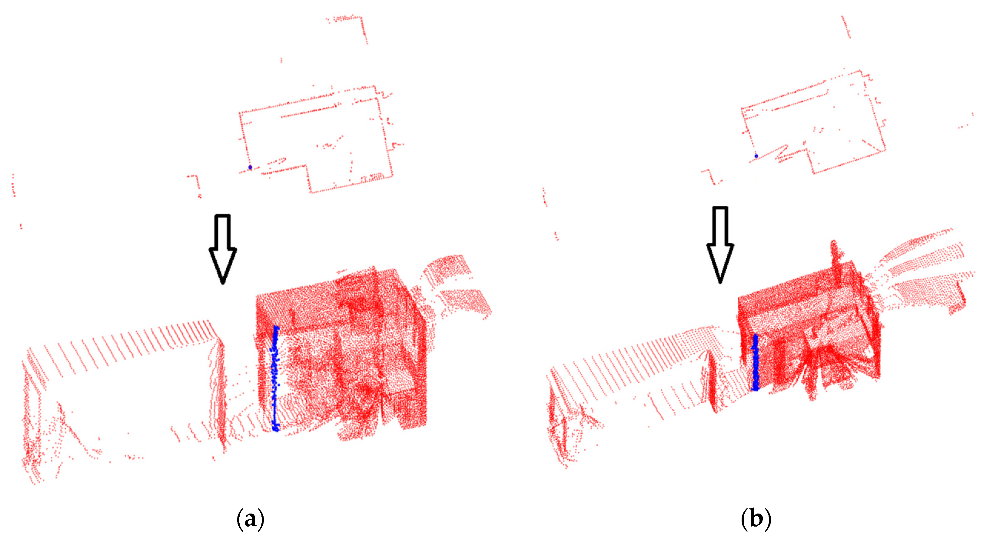
Then, the points in the overlap area are extracted from ${\overline{\mathit{P}}}_{Line-s}^s$. For a point ${\overline{\mathit{P}}}_{Line-s}^s$ in the overlap area, we find its corresponding point ${\mathit{p}}_{Line-s}^s$ in ${\mathit{P}}_{Line-s}^s$. Then, a vertical cylindrical neighborhood around the point ${\mathit{p}}_{Line-s}^s$ is used to extract the neighboring points $\mathit{N}\left({\mathit{P}}_{\mathit{L}ine-s}^s\right)$ from the source point cloud ${\mathit{P}}^s$, as shown in Figure 3a. Similarly, a vertical cylindrical neighborhood around ${\overline{\mathit{P}}}_{\mathit{L}ine-s}^s$ is also used to extract the neighboring points $\mathit{N}({\overline{\mathit{P}}}_{Line-s}^s)$ from the target point cloud ${\mathit{p}}^t$, as shown in Figure 3b. Thus, we can use the minimum z-values in the two cylindrical neighborhoods to calculate the displacement

$$t_z=z_{\min }^t-z_{\min }^s$$

(11)

where $z_{min}^t$ is the minimum z-value of $\mathit{N}({\overline{\mathit{p}}}_{Line-s}^s)$, and $z_{min}^s$ is the minimum z-value of $\mathit{N}\left({\mathit{p}}_{Line-s}^s\right)$. As long as the lower parts of the two cylindrical neighborhoods are not missed, the displacement can be correctly computed. In most cases, this can be guaranteed when the point ${\overline{\mathit{p}}}_{Line-s}^s$ is one in the overlap area. In order to get the reliable displacement, we randomly select 50 points from the overlap area, and calculate 50 displacements. Then, a clustering method is performed on these displacements. The displacements with similar size will be clustered together. The false displacements are less likely to cluster together, meaning that a displacement represents a cluster. The cluster with the maximum number of the displacements is used to get the final displacement, which is the mean value of the displacements in the maximal cluster. Eventually, the 3D transformation is obtained by Equation (9). Because the lower parts of two cylindrical neighborhoods are applied to calculate the displacement, our method is not suitable for the aerial point clouds, for which the lower parts are always missed.

4. Experiments and Results

In this section, the experiments will be performed on an indoor dataset and an outdoor dataset. In order to save time, we first perform the point cloud simplification. A point-based method and a plane-based method are implemented for comparison. In the point-based method, the intrinsic shape signature (ISS) detector [40] is used to extract the keypoints, and the QLCI descriptors [14] are calculated on the keypoints. The nearest neighbor similarity ratio (NNSR) [41] is applied to establish the point-to-point correspondences. The 1-point RANSAC algorithm [41], which is an improved version of RANSAC, is applied to find the correct correspondences and calculate the 3D transformation. For the plane-based method, a similar pipeline to our method is applied for a fair comparison. The 3D planes are extracted by the region growing method in [38], then the cosine values of the normals of three planes are calculated to find the candidate plane correspondences and the triplets with parallel planes are eliminated. All the triplets are traversed to identify the correct plane correspondences and compute the 3D transformation. All the experiments are implemented in Matlab by a PC with an Intel Core i7-7500U 2.7 GHz CPU and 20 GB of RAM.

4.1. Evaluation Criterion of Registration Accuracy

Three metrics are used to evaluate the registration accuracy. The rotation error is measured by

$$e_{\mathit{R}}=acos\left(\frac{trace({\mathit{R}}_{true}\left(\mathit{R}{)}^{-1}\right)-1}{2}\right)\frac{180}{\pi }$$

(12)

where $\mathit{R}$ is the calculated rotation matrix, and ${\mathit{R}}_{true}$ is the true rotation matrix. Considering that the displacement along z-axis is separately computed in our method, we divide the translation error into horizontal error and vertical error, which are defined as

$$e_{{\mathit{T}}_h}=\left|\right|{\mathit{t}}_{true}-\mathit{t}\left|\right|$$

(13)

$$e_{{\mathit{T}}_v}=\left|\right|t_{z-true}-t_z\left|\right|$$

(14)

where $\mathit{t}$ is the calculated 2D translation vector, ${\mathit{t}}_{true}$ is the true 2D translation vector, $t_z$ is the calculated displacement along z-axis, and $t_{z-true}$ is the true displacement along z-axis. Here, the true values ${\mathit{R}}_{true}$, ${\mathit{t}}_{true}$ and $t_{z-true}$ are obtained by the fine registration, which is performed by the ICP algorithm [10].

4.2. Registration Results on the Indoor Dataset

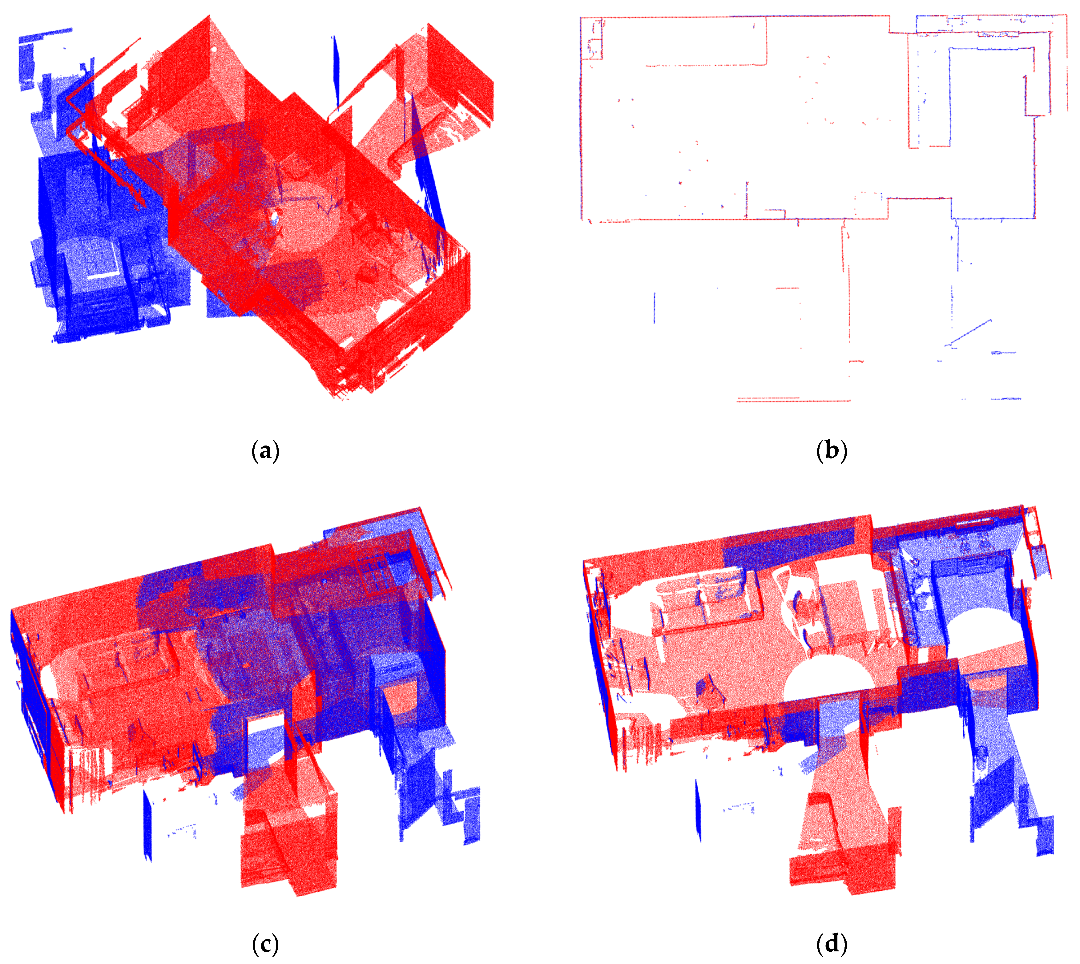
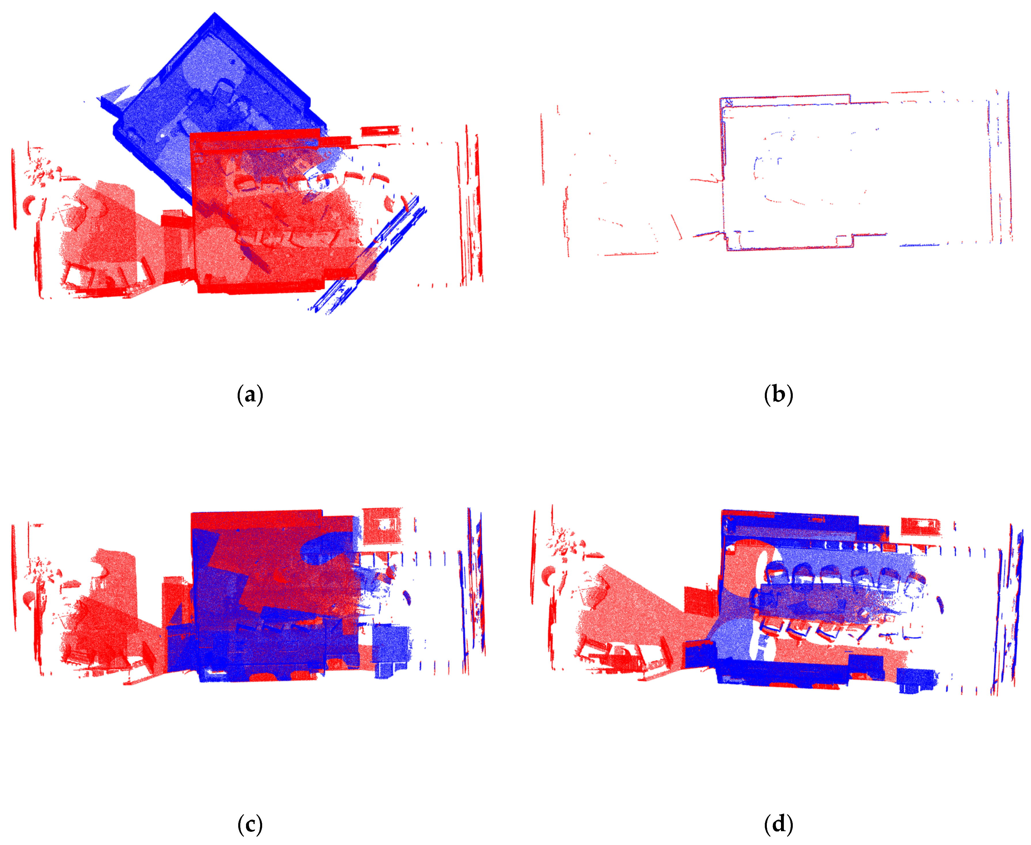
The indoor dataset [42] is acquired by a FARO Focus 3D X330 HDR scanner. The publishers scanned five scenes: Apartment, Bedroom, Boardroom, Lobby and Loft. For each scene, multiple point clouds were obtained from different views. We choose the two point clouds of Apartment and two point clouds of Boardroom to perform the experiments. The registration results obtained by our method are shown in Figure 4 and Figure 5. In order to have a better visual experience, we remove the points on the ceiling after two point clouds are registered and exhibit the point clouds without the points on the ceiling.

As we can see from Figure 4 and Figure 5, the two point clouds of both Apartment and Boardroom are automatically aligned. There is no significant inconsistency between the two registered point clouds. The simplified 2D point clouds are quite well aligned together. From the indoor furniture (e.g., sofa and chair in Figure 4d, and the council board and meeting chair in Figure 5), we can further see that the registration results are rather good.

The registration accuracy of the three methods is shown in

Table 1. The registration accuracy of the three methods on the indoor dataset. The best results are denoted in bold font.

Method	Point-Based		Plane-Based		Ours
	Ap	Bo	Ap	Bo	Ap	Bo
Rotation error	0.9756	0.2798	0.1454	0.2533	0.0560	0.5219
Horizontal error	0.3933	0.3363	0.0360	0.1961	0.0119	0.0542
Vertical error	0.0367	0.0244	0.0101	0.0163	0.0035	0.0047

. In order to save space, Apartment is abbreviated as Ap, and Boardroom is abbreviated as Bo. We can see that all the three methods can provide enough good initial pose for the fine registration. Our method obtains the best registration accuracy. The point-based method is the poorest method. This is because the point-based method is sensitive to noise and point density variation. The 3D plane and 2D line belong to the higher-level geometric feature, so the plane-based and 2D line-based methods can achieve significantly more accurate registration results. The plane-based method shows inferior registration accuracy compared to our method. This is because the region growing method [38] is not robust to outliers, meaning that the fitting accuracy of plane is low. In contrast, the distance indicator is applied in our 2D line extraction method. The outliers can be removed automatically. For the vertical error, our method also gets the smallest error. This indicates that the proposed method for calculating the displacement along the z-axis is feasible.

The computation time of the three methods is listed in the

Table 2. The number of features and the time spent on each phase for the three methods on the indoor dataset. $T_E$ denotes the time for feature extraction, $T_{\mathit{c}}$ denotes the time for coarse registration, $T_F$ denotes the time for fine registration, and $T_T$ denotes the total time.

Method	Point-Based		Plane-Based		Ours
	Ap	Bo	Ap	Bo	Ap	Bo
Number of features	2892 vs. 4255	2073 vs. 2878	20 vs. 15	17 vs. 25	31 vs. 33	23 vs. 27
$T_E$ (s)	190.6316	56.7230	1239.3671	531.2027	6.6306	4.7974
$T_{\mathit{c}}$ (s)	527.4623	374.7924	184.3647	393.2501	82.2310	38.9694
$T_F$ (s)	142.7769	70.0760	31.7702	134.0434	86.5453	71.3934
$T_T$ (s)	860.8708	501.5914	1455.5020	1058.4962	175.4069	115.1602

. In the Apartment scene, the number of points in the source and target point clouds is 124,426 and 185,436, respectively. In the Boardroom scene, the number of points in the two point clouds is 101,276 and 138,880, respectively. We also give the numbers of the features of the two point clouds being matched for better comparison. The feature in the three methods respectively denotes point feature (i.e., keypoint), plane feature and 2D line feature. Because the accuracy of the coarse registration has a great influence on the iteration number of the fine registration, we also give the computation time for the fine registration. For the plane-based method, we also set a threshold of the minimum fitting residual to stop the feature extraction. Actually, the numbers of the extracted plane features are 65 vs. 77 for Apartment and 87 vs. 108 for boardroom. In this experiment, we only use the large planes to calculate the 3D transformation. Nevertheless, we can see from Table 2 that the computation time for the feature extraction in the plane-based method is much more than that in our method. The plane-based method extracts the 3D planes and processes the point clouds in 3D space. As consequence, the computation cost is very high. By contrast, in our method, only the points with high density are extracted and further simplified to reduce the number of the points. Finally, the 2D lines are extracted in 2D space. Thus, our feature extraction is computationally very efficient. The time cost of the coarse registration in the plane-based method is also significantly more than that in our method, though the plane-based method has less features and our method has an additional step to calculate the displacement along the z-axis. This is because the number of the formed triplets in the plane-based method is much more than the number of the formed pairs in our method. The point-based method is also more time-consuming than our method, because the number of the keypoints is big. Processing thousands of keypoints needs a great deal of computation cost. The 1-point RANSAC algorithm uses the local reference frames of keypoints to calculate the rotation, so only one point is enough to calculate the 3D transformation. This largely reduces the required iteration number of the RANSAC algorithm. In this experiment, the iteration number is set as 200, but the point-based method still spends more time on the coarse registration than our method.

4.3. Registration Results on the Outdoor Dataset

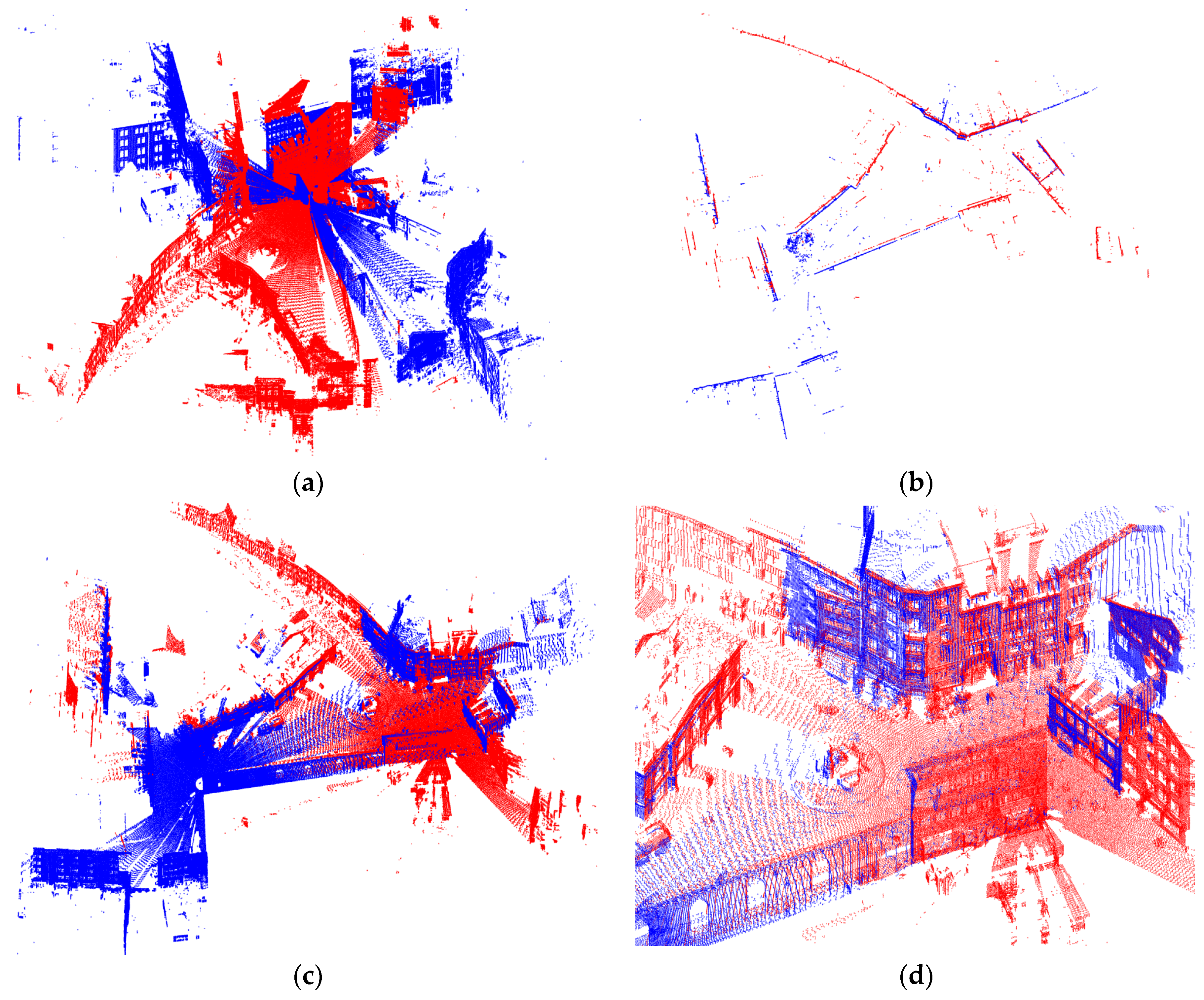
The outdoor dataset [43] is acquired by a Leica C10 laser scanner. The publishers provide the point clouds of the City and Castle scenes. We choose two point clouds from each scene to perform the experiments. The experimental results obtained by our method are shown in Figure 6 and Figure 7. We also amplify the local point clouds in order to see the registration results more clearly.

For the outdoor scenes, our method is still feasible. The simplified 2D point clouds are aligned quite well. We can also see from the registration results of the 3D point clouds (Figure 6c and Figure 7c) and the locally amplified point clouds (Figure 6d and Figure 7d) that the point clouds of both the two scenes are well registered.

The registration accuracy tested on the outdoor dataset is listed in

Table 3. The registration accuracy of the three methods on the outdoor dataset. The best results are denoted in bold font.

Method	Point-Based		Plane-Based		Ours
	City	Castle	City	Castle	City	Castle
Rotation error	2.0206	8.2586	0.7600	1.8412	0.0013	0.1813
Horizontal error	0.3091	1.2927	0.2877	0.5308	0.2319	0.1109
Vertical error	0.6536	2.6860	0.3485	0.0443	0.0088	0.0119

. Our method obtains the highest accuracy, followed by the plane-based method and point-based method. Due to the sensitivity to noise and point density variation, the point-based method achieves the poorest accuracy. In the plane-based method, the applied plane extraction method is not able to resist outliers, so the method also exhibits a poorer registration accuracy than our method. In comparison with the other two methods, the vertical error of our method is rather small as well. This means that our method can get the precise displacement along the z-axis.

The time efficiency tested on the outdoor dataset is listed in

Table 4. The number of features and the time spent on each phase for the three methods on the outdoor dataset. $T_E$ denotes the time for feature extraction, $T_{\mathit{c}}$ denotes the time for coarse registration, $T_F$ denotes the time for fine registration, and $T_T$ denotes the total time.

Method	Point-based		Plane-based		Ours
	City	Castle	City	Castle	City	Castle
Number of features	2627 vs. 2632	14,778 vs. 11,482	29 vs. 42	44 vs. 37	32 vs. 48	55 vs. 52
$T_E$ (s)	195.9942	1260.3	1958.3	8175.8	10.4173	23.3062
$T_{\mathit{c}}$ (s)	558.7629	4244.7	1696.0	6377.4	123.9002	506.9736
$T_F$ (s)	105.3999	2601.5	77.4270	915.0109	68.6787	183.1849
$T_T$ (s)	860.1570	8106.5	3731.7	15468.3	202.9962	713.4647

. In the City scene, the number of points in the source and target point clouds is 193,219 and 177,535, respectively. In the Castle scene, the number of points in the two point clouds is 455,367 and 426,357, respectively. The exact numbers of the extracted planes in the plane-based method are 160 vs. 172 for City and 158 vs. 157 for Castle. Only the large planes are used to perform the point cloud registration. As we can see, our method achieves the best computation efficiency. The plane-based method is the most time-consuming, because it processes the point clouds in 3D space. The point-based method is also computationally expensive due to the large number of the keypoints. Specially, for the Castle scene, the number of the extracted keypoints is very large. This is because the ISS detector prefers to extract the points with abundant geometric information (i.e., non-planar points) as the keypoints, and there is a large amount of such points (e.g., the points of the trees) in the scene.

5. Conclusions

In this paper, we presented a registration method based on the 2D line features. Firstly, a 2D line extraction algorithm was proposed. Then, the simplified 2D point clouds were registered by establishing correspondences between the 2D lines from the two point clouds being matched, and the 2D transformation was calculated. Finally, a method was formulated to compute the displacement along the z-axis, and the 3D transformation was obtained by integrating the 2D transformation and displacement.

The experiments have been performed on an indoor dataset and an outdoor dataset to validate the performance of our method. A point-based method and a plane-based method are compared with our method. The experimental results show that our method can obtain a relatively good registration result. In terms of the registration accuracy, our method is the best on both of the two datasets. The rotation error is less than 0.55^o. The horizontal error is less than 0.25m and the vertical error is less than 0.015m. The more significant advantage is that our method has a very good computation efficiency. On the point clouds of the Castle scene, the total computation time is the largest, which is less than 12 minutes.

References

1. Dong, Z.; Yang, B.; Liang, F.; Huang, R.; Scherer, S. Hierarchical registration of unordered TLS point clouds based on binary shape context descriptor. ISPRS J. Photogramm. Remote Sens. 2018, 144, 61–79. [Google Scholar] [CrossRef]
2. Choi, S.; Zhou, Q.; Koltun, V. Robust reconstruction of indoor scenes. In Proceedings of the IEEE Conference on Computer Vision and Pattern Recognition (CVPR), Boston, MA, USA, 7–12 June 2015; pp. 5556–5565. [Google Scholar]
3. Chen, X.; Yu, K.; Wu, H. Determination of minimum detectable deformation of terrestrial laser scanning based on error entropy model. IEEE Trans. Geosci. Remote Sens. 2018, 56, 105–116. [Google Scholar] [CrossRef]
4. Kusari, A.; Glennie, C.L.; Brooks, B.A.; Ericksen, T.L. Precise registration of laser mapping data by planar feature extraction for deformation monitoring. IEEE Trans. Geosci. Remote Sens. 2019, 57, 3404–3422. [Google Scholar] [CrossRef]
5. Zang, Y.; Yang, B.; Li, J.; Guan, H. An accurate TLS and UAV image point clouds registration method for deformation detection of chaotic hillside areas. Remote Sens. 2019, 11, 647. [Google Scholar] [CrossRef] [Green Version]
6. Awrangjeb, M.; Gilani, S.A.N.; Siddiqui, F.U. An effective data-driven method for 3-D building roof reconstruction and robust change detection. Remote Sens. 2018, 10, 1512. [Google Scholar] [CrossRef] [Green Version]
7. Yang, B.; Zang, Y. Automated registration of dense terrestrial laser-scanning point clouds using curves. ISPRS J. Photogramm. Remote Sens. 2014, 95, 109–121. [Google Scholar] [CrossRef]
8. Remondino, F. Heritage recording and 3D modeling with photogrammetry and 3D scanning. Remote Sens. 2011, 3, 1104–1138. [Google Scholar] [CrossRef] [Green Version]
9. Xu, Z.; Xu, E.; Wu, L.; Liu, S.; Mao, Y. Registration of terrestrial laser scanning surveys using terrain-invariant regions for measuring exploitative volumes over open-pit mines. Remote Sens. 2019, 11, 606. [Google Scholar] [CrossRef] [Green Version]
10. Besl, P.J.; McKay, D.N. A method for registration of 3-D shapes. IEEE Trans. Pattern Anal. Mach. Intell. 1992, 14, 239–256. [Google Scholar] [CrossRef]
11. Tao, W.; Hua, X.; Yu, K.; He, X.; Chen, X. An improved point-to-plane registration method for terrestrial laser scanning data. IEEE Access 2018, 6, 48062–48073. [Google Scholar] [CrossRef]
12. Li, W.; Song, P. A modified ICP algorithm based on dynamic adjustment factor for registration of point cloud and CAD model. Pattern Recognit. Lett. 2015, 65, 88–94. [Google Scholar] [CrossRef]
13. Rusu, R.B.; Blodow, N.; Beetz, M. Fast Point Feature Histograms (FPFH) for 3D registration. In Proceedings of the 2009 IEEE International Conference on Robotics and Automation, Kobe, Japan, 12–17 May 2009. [Google Scholar]
14. Tao, W.; Hua, X.; Wang, R.; Xu, D. Quintuple local coordinate images for local shape description. Photogramm. Eng. Remote Sens. 2020, 86, 121–132. [Google Scholar] [CrossRef]
15. Yang, J.; Xiao, Y.; Cao, Z. Aligning 2.5D scene fragments with distinctive local geometric features and voting-based correspondences. IEEE Trans. Circuits Syst. Video Technol. 2019, 29, 714–729. [Google Scholar] [CrossRef]
16. Quan, S.; Ma, J.; Hu, F.; Fang, B.; Ma, T. Local voxelized structure for 3D binary feature representation and robust registration of point clouds from low-cost sensors. Inf. Sci. 2018, 444, 153–171. [Google Scholar] [CrossRef]
17. Aiger, D.; Mitra, N.J.; Cohen-Or, D. 4-points congruent sets for robust pairwise surface registration. ACM Trans. Graph. 2008, 27, 1–10. [Google Scholar] [CrossRef] [Green Version]
18. Mellado, N.; Aiger, D.; Mitra, N.J. Super 4PCS fast global point cloud registration via smart Indexing. Eurogr. Symp. Geom. Process. 2014, 33, 205–215. [Google Scholar] [CrossRef] [Green Version]
19. Theiler, P.W.; Wegner, J.D.; Schindler, K. Keypoint-based 4-points congruent sets-automated marker-less registration of laser scans. ISPRS J. Photogramm. Remote Sens. 2014, 96, 149–163. [Google Scholar] [CrossRef]
20. Ge, X. Automatic markerless registration of point clouds with semantic-keypoint-based 4-points congruent sets. ISPRS J. Photogramm. Remote Sens. 2017, 130, 344–357. [Google Scholar] [CrossRef] [Green Version]
21. Yang, B.; Dong, Z.; Liang, F.; Liu, Y. Automatic registration of large-scale urban scene point clouds based on semantic feature points. ISPRS J. Photogramm. Remote Sens. 2016, 113, 43–58. [Google Scholar] [CrossRef]
22. Al-Durgham, K.; Habib, A.; Kwak, E. RANSAC Approach for automated registration of terrestrial laser scans using linear features. ISPRS Ann. Photogramm. Remote Sens. Spat. Inf. Sci. 2013, II-5/W2, 11–18. [Google Scholar] [CrossRef] [Green Version]
23. Al-Durgham, K.; Habib, A. Association-matrix-based sample consensus approach for automated registration of terrestrial laser scans using linear features. Photogramm. Eng. Remote Sens. 2014, 80, 1029–1039. [Google Scholar] [CrossRef]
24. Xiao, J.; Adler, B.; Zhang, J. Planar segment based three-dimensional point cloud registration in outdoor environments. J. Field Robot. 2013, 30, 552–582. [Google Scholar] [CrossRef]
25. Pathak, K.; Birk, A.; Vaškevicius, N.; Poppinga, J. Fast registration based on noisy planes with unknown correspondences for 3D mapping. IEEE Trans. Robot. 2010, 26, 424–441. [Google Scholar] [CrossRef] [Green Version]
26. Xiao, J.; Adler, B.; Zhang, H. 3D point cloud registration based on planar surfaces. In Proceedings of the 2012 IEEE International Conference on Multisensor Fusion and Integration for Intelligent Systems (MFI), Hamburg, Germany, 13–15 September 2012. [Google Scholar]
27. Xu, Y.; Boerner, R.; Yao, W.; Hoegner, L.; Stilla, U. Pairwise coarse registration of point clouds in urban scenes using voxel based 4-planes congruent sets. ISPRS J. Photogramm. Remote Sens. 2019, 151, 106–123. [Google Scholar] [CrossRef]
28. Pathak, K.; Birk, A.; Vaskevicius, N.; Pfingsthorn, M.; Schwertfeger, S.; Poppinga, J. Online three-dimensional SLAM by registration of large planar surface segments and closed-form pose-graph relaxation. J. Field Robot. 2010, 27, 52–84. [Google Scholar] [CrossRef]
29. Fan, W.; Shi, W.; Xiang, H.; Ding, K. A novel method for plane extraction from low-resolution inhomogeneous point clouds and its application to a customized low-cost mobile mapping system. Remote Sens. 2019, 11, 2789. [Google Scholar] [CrossRef] [Green Version]
30. Stamos, I.; Leordeanu, M. Automated feature-based range registration of urban scenes of large scale. In Proceedings of the 2003 IEEE Computer Society Conference on Computer Vision and Pattern Recognition, Madison, WI, USA, 18–20 June 2003; p. 555. [Google Scholar]
31. Yao, J.; Ruggeri, M.R.; Taddei, P.; Sequeira, V. Automatic scan registration using 3D linear and planar Features. 3DR Res. 2011, 6, 1–18. [Google Scholar] [CrossRef]
32. Rabbani, T.; Dijkman, S.; van den Heuvel, F.; Vosselman, G. An integrated approach for modelling and global registration of point clouds. ISPRS J. Photogramm. Remote Sens. 2007, 61, 355–370. [Google Scholar] [CrossRef]
33. Chan, T.O.; Lichti, D.D.; Belton, D.; Nguyen, H.L. Automatic point cloud registration using a single octagonal lamp pole. Photogramm. Eng. Remote Sens. 2016, 82, 257–269. [Google Scholar] [CrossRef]
34. Iman Zolanvari, S.M.; Laefer, D.F. Slicing method for curved facade and window extraction from point clouds. ISPRS J. Photogramm. Remote Sens. 2016, 119, 334–346. [Google Scholar] [CrossRef]
35. Li, B.; Li, Q.; Shi, W.; Wu, F. Feature extraction and modeling of urban building from vehicle-borne laser scanning data. Int. Arch. Photogramm. Remote Sens. Spat. Inf. Sci. 2004, 35, 934–939. [Google Scholar]
36. Xia, S.; Chen, D.; Wang, R.; Li, J.; Zhang, X. Geometric primitives in LiDAR point clouds: A review. IEEE J. Sel. Top. Appl. Earth Obs. Remote Sens. 2020, 13, 685–707. [Google Scholar] [CrossRef]
37. Xiao, J.; Zhang, J.; Zhang, J.; Zhang, H.; Hildre, H.P. Fast plane detection for SLAM from noisy range images in both structured and unstructured environments. In Proceedings of the 2011 IEEE International Conference on Mechatronics and Automation, Beijing, China, 7–10 August 2011; pp. 1768–1773. [Google Scholar]
38. Rabbani, T.; van den Heuvel, F.A.; Vosselman, G. Segmentation of point clouds using smoothness constraint. Int. Arch. Photogramm. Remote. Sens. Spat. Inf. Sci. 2006, 36, 248–253. [Google Scholar]
39. Fischler, M.A.; Bolles, R.C. Random sample consensus: A paradigm for model fitting with applications to image analysis and automated cartography. Grap. Image Process. 1981, 381–395. [Google Scholar] [CrossRef]
40. Zhong, Y. Intrinsic shape signatures: A shape descriptor for 3d object recognition. In Proceedings of the 2009 IEEE 12th International Conference on Computer Vision Workshops, Kyoto, Japan, 27 September–4 October 2009; pp. 689–696. [Google Scholar]
41. Guo, Y.; Bennamoun, M.; Sohel, F.; Lu, M.; Wan, J. An integrated framework for 3-D modeling, object detection, and pose estimation from point-clouds. IEEE Trans. Instrum. Meas. 2015, 64, 683–693. [Google Scholar] [CrossRef]
42. Park, J.; Zhou, Q.; Koltun, V. Colored point cloud registration revisited. In Proceedings of the 2017 IEEE International Conference on Computer Vision (ICCV), Venice, Italy, 22–29 October 2017; pp. 143–152. [Google Scholar]
43. Zeisl, B.; Koeser, K.; Pollefeys, M. Automatic registration of RGB-D scans via salient directions. In Proceedings of the 2013 IEEE International Conference on Computer Vision, Sydney, Australia, 1–8 December 2013; pp. 2805–2815. [Google Scholar]
Figure 1. The process of extracting the points on 2D lines. (a) The original point cloud, (b) 2D point cloud obtained by projecting the original point cloud on the horizontal plane, (c) the points with high point density are extracted.
Remotesensing 12 01283 g001
Figure 2. The outline of our registration method.
Remotesensing 12 01283 g002
Figure 3. The illustration of the extraction of the points in the cylindrical neighborhood. The blue points are the extracted points by using the cylindrical neighborhood. (a) The simplified 2D point cloud P L i n e s s and the source point cloud P s , (b) the simplified 2D point cloud P L i n e s t and the target point cloud P t .
Remotesensing 12 01283 g003
Figure 4. The coarse registration result of Apartment. (a) The source and target point clouds. (b) The registration result of the simplified 2D point clouds. (c) The registration result of the 3D point clouds. (d) The registered point clouds after removing the points on the ceiling for a better view.
Remotesensing 12 01283 g004
Figure 5. The coarse registration result of Boardroom. (a) The source and target point clouds. (b) The registration result of the simplified 2D point clouds. (c) The registration result of the 3D point clouds. (d) The registered point clouds after removing the points on the ceiling for a better view.
Remotesensing 12 01283 g005
Figure 6. The coarse registration result of City. (a) The source and target point clouds. (b) The registration result of the simplified 2D point clouds. (c) The registration result of the 3D point clouds. (d) The locally amplified point clouds for a better view.
Remotesensing 12 01283 g006
Figure 7. The coarse registration result of Castle. (a) The source and target point clouds. (b) The registration result of the simplified 2D point clouds. (c) The registration result of the 3D point clouds. (d) The locally amplified point clouds for a better view.
Remotesensing 12 01283 g007