An Integrated Shadow-Adjusted Snow-Aging Index for Alpine Regions


Abstract

1. Introduction
2. Study Area and Data
2.1. Study Area
2.2. Satellite and Auxiliary Data
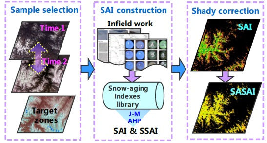
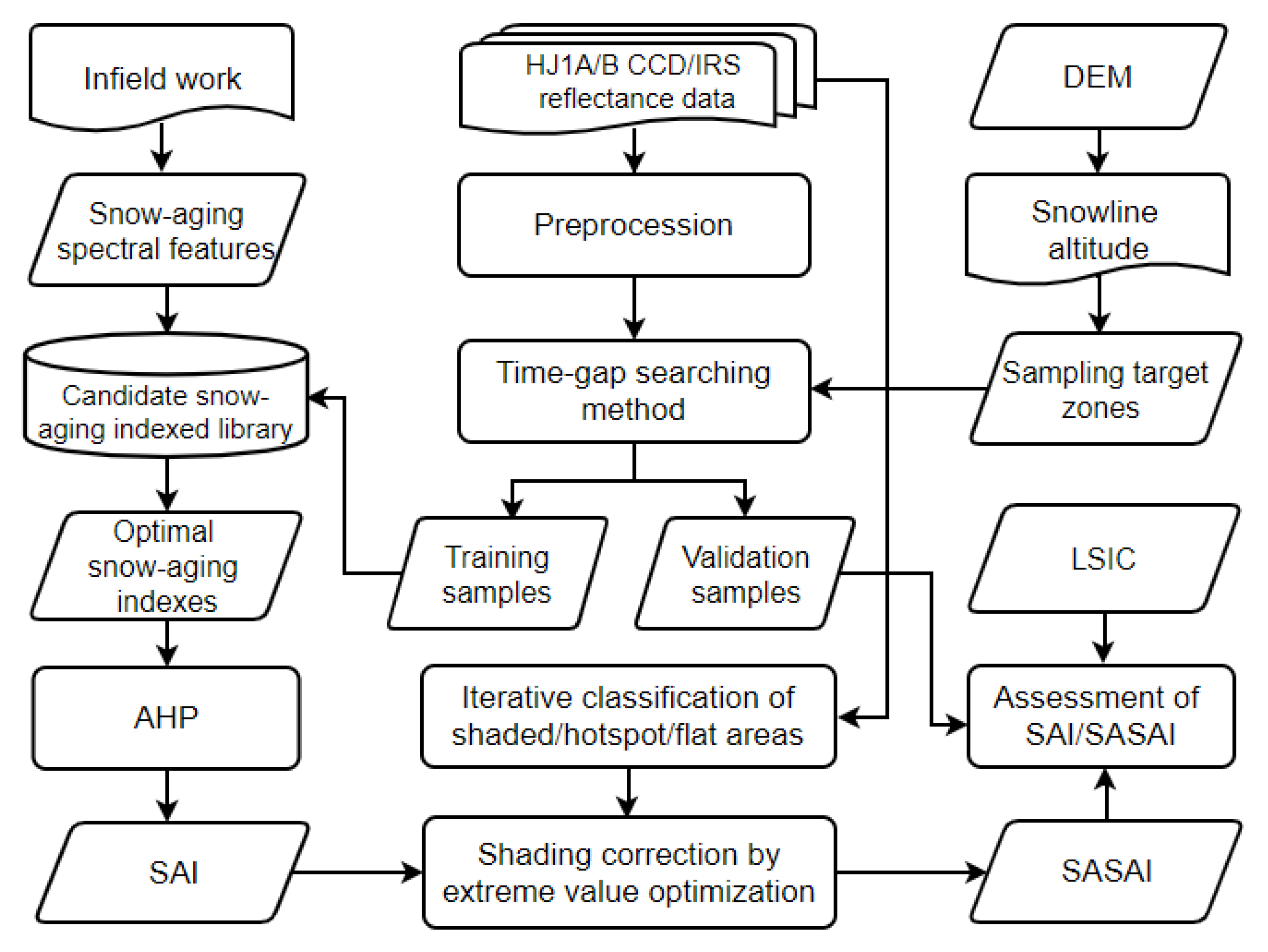
3. Methods
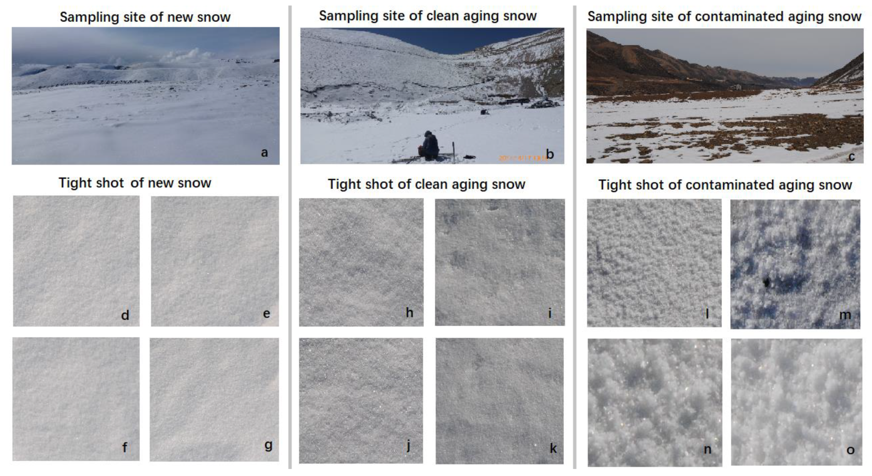
3.1. Field Work
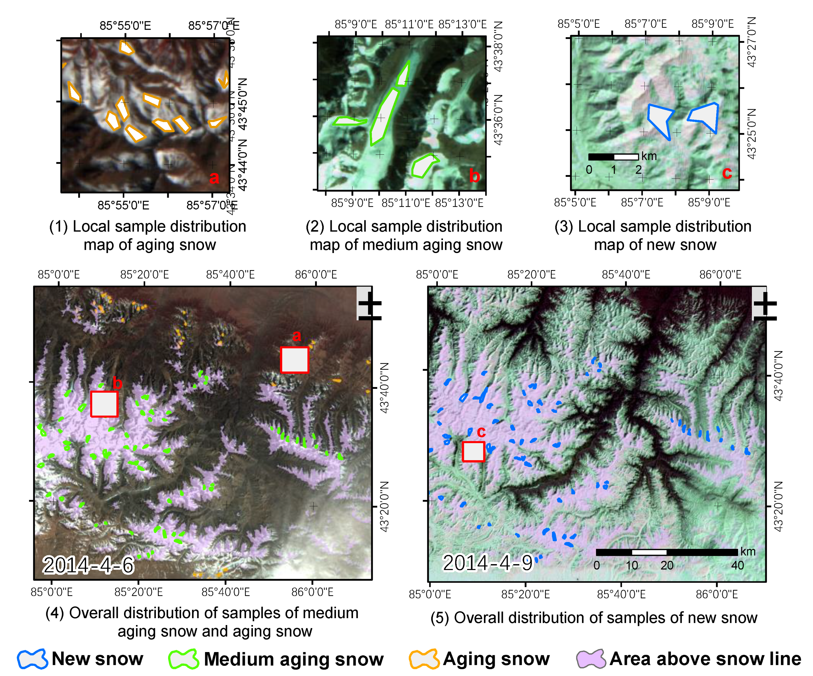
3.2. “Time-Gap Searching” for Snow-Aging Samples
3.3. Analytic Hierarchy Process for Construction of the SAI
3.4. Elimination of the Terrain-Induced Shadow Effect
4. Results
4.1. Field Measurements and Analyses
4.2. Optimized Snow Cover Aging Indexes
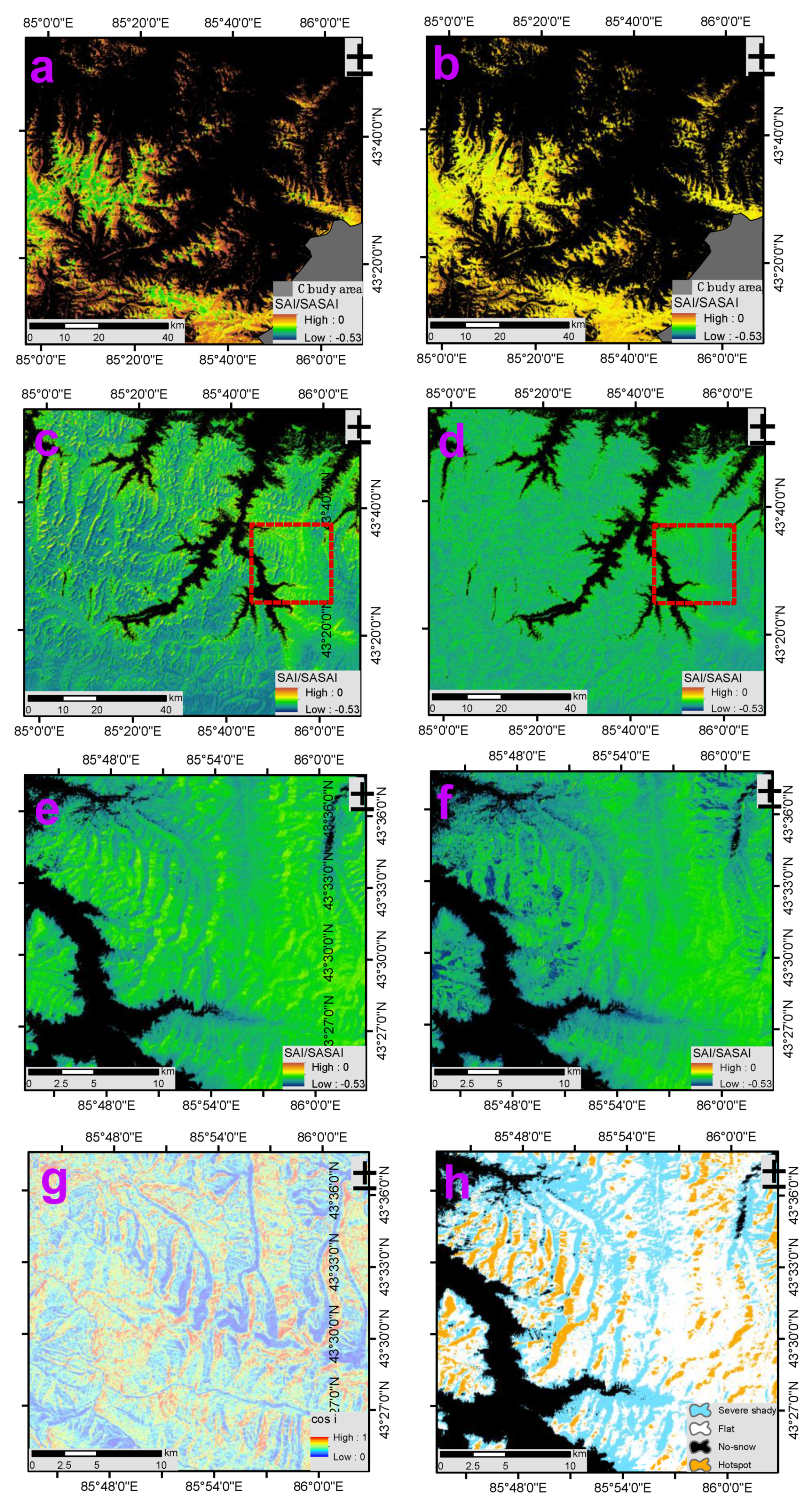
4.3. Snow-Aging Index (SAI) and Shadow-Adjusted Snow-Aging Index (SASAI)
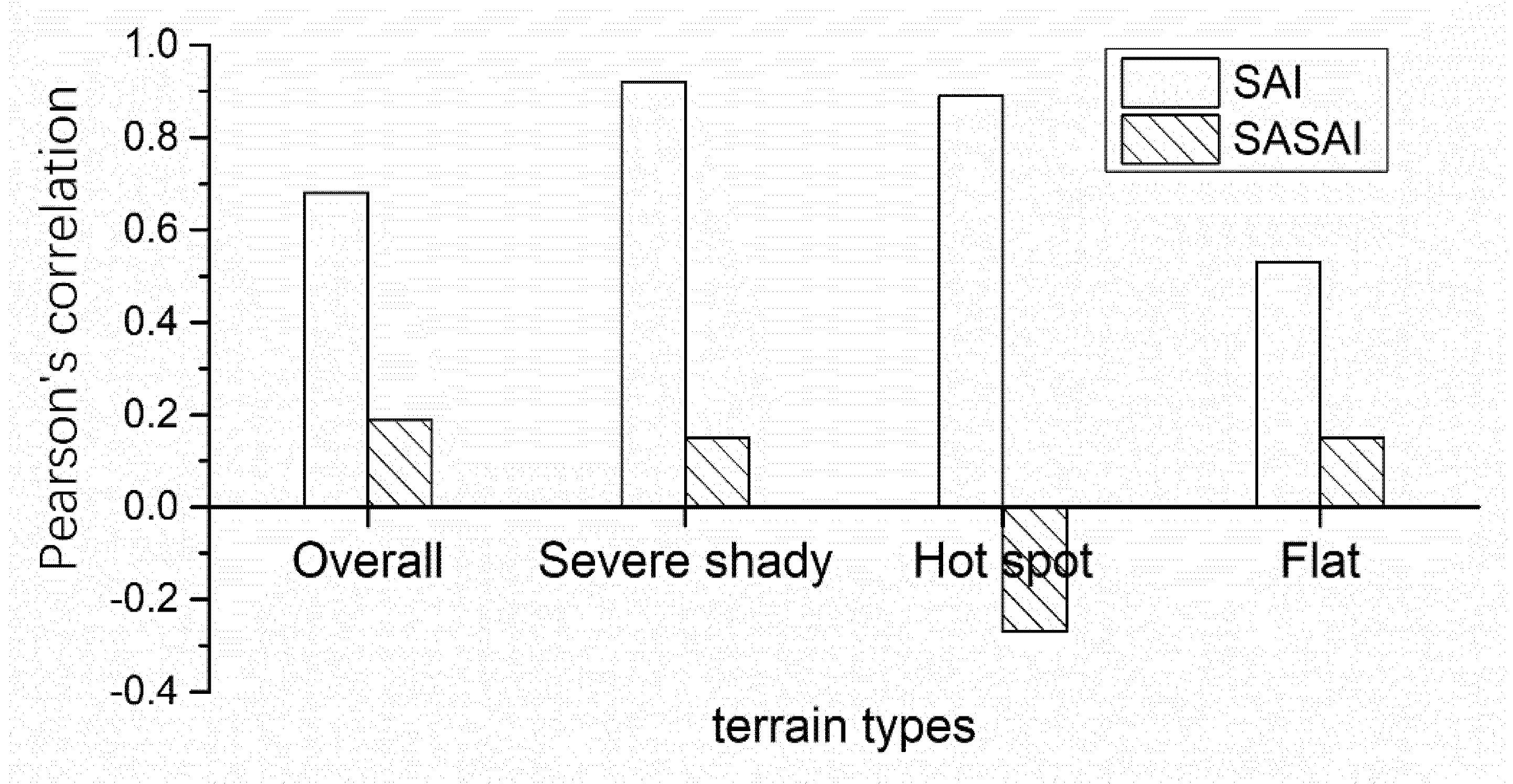
4.4. Assessment of the Shading Correction and Accuracy of SAI/SASAIs
5. Discussion
6. Conclusions
Author Contributions
Funding
Acknowledgments
Conflicts of Interest
References
- Bartolini, E.; Adam, J.; Claps, P. Global snow cover: Comparison of modeling results with satellite-derived snow cover maps. In Proceedings of the AGU Fall Meeting, San Francisco, CA, USA, 13–17 December 2010. [Google Scholar]
- Meyer, C.R.; Hewitt, I.J. A continuum model for meltwater flow through compacting snow. Cryosphere 2017, 11, 2799–2813. [Google Scholar] [CrossRef]
- Steger, C.; Kotlarski, S.; Jonas, T.; Schär, C. Alpine snow cover in a changing climate: A regional climate model perspective. Clim. Dyn. 2013, 41, 735–754. [Google Scholar] [CrossRef]
- Colbeck, S.C. An overview of seasonal snow metamorphism. Rev. Geophys. 1982, 20, 45–63. [Google Scholar] [CrossRef]
- Martinec, J.; Rango, A. Parameter values for snowmelt runoff modelling. J. Hydrol. 1986, 84, 197–219. [Google Scholar] [CrossRef]
- Hall, D.K.; Martinec, J. Remote Sensing of Ice and Snow; Chapman and Hall: London, UK, 1985. [Google Scholar]
- Salomonson, V.V.; Hall, D.K.; Chien, J.Y.L. Use of passive microwave and optical data for large-scale snow-cover mapping. In Proceedings of the Symposium on Combined Optical-Microwave Earth & Atmosphere Sensing, Atlanta, GA, USA, 3–6 April 1995. [Google Scholar]
- Hall, D.K.; Riggs, G.A.; Foster, J.L.; Kumar, S.V. Development and evaluation of a cloud-gap-filled MODIS daily snow-cover product. Remote Sens. Environ. 2010, 114, 496–503. [Google Scholar] [CrossRef]
- Painter, T.H.; Andreadis, K.; Berisford, D.F.; Goodale, C.E.; Hart, A.F.; Heneghan, C. The Airborne Snow Observatory: Fusion of imaging spectrometer and scanning lidar for studies of mountain snow cover (Invited). In Proceedings of the AGU Fall Meeting, San Francisco, CA, USA, 9–13 December 2013. [Google Scholar]
- Jing, Y.; Shen, H.; Li, X.; Guan, X. A Two-Stage Fusion Framework to Generate a Spatio–Temporally Continuous MODIS NDSI Product over the Tibetan Plateau. Remote Sens. 2019, 11, 2261. [Google Scholar] [CrossRef]
- Li, X.; Jing, Y.; Shen, H.; Zhang, L. The recent developments in cloud removal approaches of MODIS snow cover product. Hydrol. Earth Syst. Sci. 2019, 23, 2401–2416. [Google Scholar] [CrossRef]
- Harrison, A.; Lucas, R. Multi-spectral classification of snow using NOAA AVHRR imagery. Int. J. Remote Sens. 1989, 10, 907–916. [Google Scholar] [CrossRef]
- Hall, D.K.; Riggs, G.A.; Salomonson, V.V.; DiGirolamo, E.N.; Bayr, K.J. Modis snow-cover products. Remote Sens. Environ. 2002, 83, 181–194. [Google Scholar] [CrossRef]
- Ahmad, M.; Khan, A.; Tariq, S.; Blaschke, T. Contrasting changes in snow cover and its sensitivity to aerosol optical properties in Hindukush-Karakoram-Himalaya region. Sci. Total Environ. 2019, 699, 134356. [Google Scholar] [CrossRef]
- Painter, T.H.; Rittger, K.; Mckenzie, C.; Slaughter, P.; Davis, R.E.; Dozier, J. Retrieval of subpixel snow covered area, grain size, and albedo from MODIS. Remote Sens. Environ. 2009, 113, 868–879. [Google Scholar] [CrossRef]
- Wu, T.; Wu, G. An empirical formula to compute snow cover fraction in GCMs. Adv. Atmos. Sci. 2004, 21, 529–535. [Google Scholar] [CrossRef]
- Vikhamar, D.; Solberg, R. A constrained spectral unmixing approach to snow-cover mapping in forests using MODIS data, IGARSS 2003. In Proceedings of the 2003 IEEE International Geoscience and Remote Sensing Symposium, Toulouse, France, 21–25 July 2003; Volume 2, pp. 833–835. [Google Scholar]
- Zhou, C.X.; Zheng, L. Mapping radar glacier zones and dry snow line in the Antarctic peninsula using sentinel-1 images. Remote Sens. 2013, 9, 1171. [Google Scholar] [CrossRef]
- Kim, R.S.; Durand, M.; Li, D.; Baldo, E.; Margulis, S.A.; Dumont, M. Estimating alpine snow depth by combining multifrequency passive radiance observations with ensemble snowpack modeling. Remote Sens. Environ. 2019, 226, 1–15. [Google Scholar] [CrossRef]
- Mei, L.; Xue, Y.; Leeuw, G.D.; Hoyningen-Huene, W.V.; Kokhanovsky, A.A.; Istomina, L. Aerosol optical depth retrieval in the arctic region using MODIS data over snow. Remote Sens. Environ. 2013, 128, 234–245. [Google Scholar] [CrossRef]
- Yuan, X.; Barton, A.F. Atmospheric and forest decoupling of passive microwave brightness temperature observations over snow-covered terrain in North America. IEEE J. Sel. Top. Appl. Earth Obs. Remote Sens. 2016, 10, 3172–3189. [Google Scholar]
- Chen, X.N.; Di, L.; Liang, S.L.; He, L.; Zeng, C.; Hao, X.H.; Hong, Y. Developing a composite daily snow cover extent record over the Tibetan plateau from 1981 to 2016 using multisource data. Remote Sens. Environ. 2018, 215, 284–299. [Google Scholar] [CrossRef]
- Luojus, K.; Pulliainen, J.; Takala, M.; Lemmetyinen, J.; Derksen, C.; Bojkov, B. ESA Globsnow- Hemispherical Snow Extent and Snow Water Equivalent Records for Climate Research Purposes. In Proceedings of the AGU Fall Meeting, San Francisco, CA, USA, 5–9 December 2011; Volume 6. [Google Scholar]
- Tedesco, M.; Narvekar, P.S. Assessment of the NASA AMSR-E SWE Product. IEEE J. Sel. Top. Appl. Earth Obs. Remote Sens. 2010, 3, 141–159. [Google Scholar] [CrossRef]
- Li, Z.; Li, Z.; Tian, B.; Zhou, J. An INSAR scattering model for multi-layer snow based on quasi-crystalline approximation (QCA) theory. Sci. China Earth Sci. 2018, 61, 1–15. [Google Scholar] [CrossRef]
- Negi, H.S.; Kulkarni, A.V. Effect of contamination and mixed objects on snow reflectance using spectroradiometer in Beas Basin, India. Asia-Pac. Remote Sens. Symp. 2006, 6411, 641115. [Google Scholar]
- Mishra, V.D.; Negi, H.S.; Rawat, A.K.; Chaturvedi, A.; Singh, R. Retrieval of sub-pixel snow cover information in the Himalayan region using medium and coarse resolution remote sensing data. Int. J. Remote Sens. 2009, 30, 4707–4731. [Google Scholar] [CrossRef]
- Singh, S.K.; Kulkarni, A.V.; Chaudhary, B. Hyperspectral analysis of snow reflectance to understand the effects of contamination and grain size. Ann. Glaciol. 2010, 51, 83–88. [Google Scholar] [CrossRef]
- Snapir, B.; Momblancha, A.; Jainb, S.K.; Wainea, T.W.; Holmana, I.P. A method for monthly mapping of wet and dry snow using Sentinel-1 and MODIS: Application to a Himalayan river basin. Int. J. Appl. Earth Obs. 2019, 74, 222–230. [Google Scholar] [CrossRef]
- Thomas, E.S. The Spatial Distribution of Fine Resolution Snow Surface Roughness. In Proceedings of the AGU Fall Meeting, San Francisco, CA, USA, 12–16 December 2016. [Google Scholar]
- Thakur, P.K.; Aggarwal, S.P.; Arun, G. Estimation of Snow Cover Area, Snow Physical Properties and Glacier Classification in Parts of Western Himalayas Using C-Band SAR Data. J. Indian Soc. Remote 2017, 45, 525–539. [Google Scholar] [CrossRef]
- Varade, D.; Dikshit, O.; Manickam, S. Dry/wet snow mapping based on the synergistic use of dual polarimetric SAR and multispectral data. J. Mt. Sci. 2019, 16, 1435–1451. [Google Scholar] [CrossRef]
- Zhang, T.J.; Zhong, X.Y. Classification and regionalization of the seasonal snow cover across the Eurasian continent. J. Glaciol. Geocryol. 2014, 36, 481–490. [Google Scholar]
- Ohmura, A. Physical Basis for the Temperature-Based Melt-Index Method. J. Appl. Meteorol. Clim. 2001, 40, 753–761. [Google Scholar] [CrossRef]
- Pomeroy, J.W.; Gray, D.M.; Shook, K.R.; Toth, B.; Essery, R.L.H.; Pietroniro, A. An evaluation of snow accumulation and ablation processes for land surface modelling. Hydrol. Process. 1999, 12, 2339–2367. [Google Scholar] [CrossRef]
- Ewa, B. Snow cover in Eastern Europe in relation to temperature, precipitation and circulation. Int. J. Clim. 2004, 24, 591–601. [Google Scholar]
- Sumargo, E. Cloudiness over the Mountains of the Western United States: Variability and Influences on Snowmelt and Streamflow; University of California: San Diego, CA, USA, 2018. [Google Scholar]
- Painter, T.H. The Hyperspectral Bidirectional Reflectance of Snow: Modeling, Measurement, and Instrumentation; University of California: Santa Barbara, CA, USA, 2002. [Google Scholar]
- Fontaine, T.A.; Cruickshank, T.S.; Arnold, J.G.; Hotchkiss, R.H. Development of a snowfall–snowmelt routine for mountainous terrain for the soil water assessment tool (swat). J. Hydrol. 2002, 262, 209–223. [Google Scholar] [CrossRef]
- Naha, S.; Thakur, P.K.; Aggarwal, S.P. Hydrological Modelling and data assimilation of Satellite Snow Cover Area using a Land Surface Model, VIC. In Proceedings of the ISPRS-International Archives of the Photogrammetry, Remote Sensing and Spatial Information Sciences, Prague, Czech Republic, 12–19 July 2016; Volume XLI–B8, pp. 353–360. [Google Scholar]
- Warren, S.G.; Wiscombe, W.J. A Model for the Spectral Albedo of Snow. II: Snow Containing Atmospheric Aerosols. J. Atmos. Sci. 1980, 37, 2734–2745. [Google Scholar] [CrossRef]
- Mernild, S.H.; Edward, H.; Joseph, R.M. Greenland precipitation trends in a long-term instrumental climate context (1890–2012): Evaluation of coastal and ice core records. Int. J. Clim. 2015, 352, 303–320. [Google Scholar] [CrossRef]
- Nolin, A.W. Recent advances in remote sensing of seasonal snow. J. Glaciol. 2017, 56, 1141–1150. [Google Scholar] [CrossRef]
- Chang, A.T.C.; Kelly, R.E.; Foster, J.L.; Hall, D.K. Estimation of global snow cover using passive microwave data. Proc. SPIE Int. Soc. Opt. Eng. 2003, 17, 381–390. [Google Scholar]
- Huang, J.; Lan, X.; Wang, H.; Yuan, L.; Xiao, H. Optical carrier based microwave interferometers for sensing application. Fiber Opt. Sens. Appl. XI 2014, 9098, 90980H. [Google Scholar]
- Salcode, A.P.; Cogliati, M.G. Snow Cover Area Estimation Using Radar and Optical Satellite Information. Atmos. Clim. Sci. 2014, 4, 514–523. [Google Scholar]
- Foster, J.L.; Sun, C.; Walker, J.P. Quantifying the uncertainty in passive microwave snow water equivalent observations. Remote Sens. Environ. 2005, 94, 187–203. [Google Scholar] [CrossRef]
- Zang, X.; Yang, B.; Qi, J.W.; Xiang, X.Y. An Improved Topographic Correction Method of Remote-sensing Images. Bull. Surv. Mapp. 2015, 1, 75–80. [Google Scholar]
- Yang, Y.K.; Feng, X.Z.; Xiao, P.F.; He, G.J. Spectral characteristic analysis of snow in mountainous areas of Manasi River Basin. J. Nanjing Univ. 2015, 5, 929–935. [Google Scholar]
- Feng, X.Z. Remote Sensing and Application of Snow Cover in Central Tianshan; Science Press: Beijing, China, 2018. [Google Scholar]
- Hao, X.H.; Wang, J.; Wang, J.; Zhang, P.; Huang, C.L. The measurement and retrieval of the spectral reflectance of different snow grain size on Northern Xinjiang, China. Spectrosc. Spectr. Anal. 2013, 33, 190–195. [Google Scholar]
- Ingvander, S.; Johansson, C.; Jansson, P.; Pettersson, R. Comparison of digital and manual methods of snow particle size estimation. Hydrol. Res. 2012, 43, 192–202. [Google Scholar] [CrossRef]
- Hu, R.J. Physical Geography of the Tianshan Mountains in China; China Environmental Science Press: Beijing, China, 2004. [Google Scholar]
- Saaty, T.L.; Vargas, L.G. Estimating technological coefficients by the analytic hierarchy process. Socio-Econ. Plan. Sci. 1979, 13, 333–336. [Google Scholar] [CrossRef]
- Hall, D.K.; Foster, J.L.; Chien, J.Y.L.; Riggs, G.A. Determination of actual snow-covered area using Landsat TM and digital elevation model data in Glacier National Park, Montana. Polar Rec. 1995, 31, 191–198. [Google Scholar] [CrossRef]
- Chylek, P.; Mccabe, M.; Dubey, M.K.; Dozier, J. Remote sensing of Greenland ice sheet using multispectral near-infrared and visible radiances. J. Geophys. Res. Atmos. 2007, 112. [Google Scholar] [CrossRef]
- Negi, H.S.; Kokhanovsky, A. Retrieval of snow grain size and albedo of Western Himalayan snow cover using satellite data. Cryosphere 2011, 5, 831–847. [Google Scholar] [CrossRef]
- Kour, R.; Patel, N.; Krishna, A.P. Assessment of relationship between snow cover characteristics (SGI and SCI) and snow cover indices (NDSI and S3). Earth Sci. Inform. 2015, 8, 317–326. [Google Scholar] [CrossRef]
- Shimamura, Y.; Izumi, T.; Matsuyama, H. Evaluation of a useful method to identify snow-covered areas under vegetation—Comparisons among a newly proposed snow index, normalized difference snow index, and visible reflectance. Int. J. Remote Sens. 2006, 27, 4867–4884. [Google Scholar] [CrossRef]
- Kour, R.; Patel, N.; Krishna, A.P. Development of a new thermal snow index and its relationship with snow cover indices and snow cover characteristic indices. Arab. J. Geosci. 2016, 9, 71. [Google Scholar] [CrossRef]


| Fresh Snow | Aging Snow | Contaminated Snow | |
|---|---|---|---|
| Color | Bright and clear | Bright and clear | Dull and impure |
| Shape (as shown in Figure 7) | No crystallization, snowflake, hexagon, columnar, or a mixture | Spherical and agglomerated | Spherical and agglomerated |
| Equivalent Grain size | 200 nm–300 nm | 600 nm–1000 nm | 750 nm–1200 nm |
| Average layer water content | 1.2–1.6% | 2–4% | 6–9% |
| Average density | 176–221 kg/m3 | 320–90 kg/m3 | 340–420 kg/m3 |
| Average Air temperature | −9.8 ℃ | −2.5 ℃ | 7.8 ℃ |
| Sampling date | 10–17 December 2013 | 15–22 March 2014 | 15–22 March 2014 |
| Time lag from snow fall | ~1 day | > 7 days | > 7 days |
| Index Types | Index Name | Calculation Formula | N/A | N/M | M/A |
|---|---|---|---|---|---|
| Snow cover indicator | Normalized Difference Snow Index [55] | NDSI = | 0.65 | 0.95 | 0.66 |
| Melt Area Detection Index [56] | MADI = | 1.10 | 0.98 | 0.93 | |
| Grain size indicator | Snow Grain Index [57] | SGI = | 1.29 | 1.41 | 1.41 |
| Contamination indicator | Snow Contamination Index [58] | SCI = | 0.81 | 0.75 | 0.67 |
| Vegetation indicator | S3 [59] | S3 = | 0.69 | 1.06 | 0.61 |
| Temperature indicator | Normalized Difference Temperature Snow Index [60] | NDTSI = | 1.08 | 0.98 | 0.70 |
| Normalized Difference Snow Temperature Index [60] | NDSTI = | 1.41 | 1.05 | 1.11 | |
| S3 Temperature Snow Index [60] | S3TSI = | 0.78 | 1.23 | 0.80 | |
| Single band reflectance | Reflectance of HJ-1A/B CCD band 1 | Ref Blue | 1.41 | 1.18 | 1.15 |
| Reflectance of HJ-1A/B CCD band 2 | Ref Green | 1.41 | 0.97 | 1.08 | |
| Reflectance of HJ-1A/B CCD band 3 | Ref Red | 0.73 | 1.30 | 1.33 | |
| Reflectance of HJ-1A/B CCD band 4 | Ref NIR | 1.41 | 1.11 | 0.96 | |
| HJ-1A/B CCD with spatial resolution of 30 m | HJ-1B IRS with spatial resolution of 120 m | ||||
| Blue: Band 1 (0.43–0.52 μm) | NIR: Band 5 (0.75–1.10 μm) | ||||
| Green: Band 2 (0.52–0.60 μm) | SWIR: Band 6 (1.55–1.75 μm) | ||||
| Red: Band 3 (0.63–0.69 μm) | MIR: Band 7 (3.50–3.90 μm) | ||||
| NIR: Band 4 (0.76–0.90 μm) | TIR: Band 8 (10.5–12.5 μm) | ||||
| N/A: New & Aging snow | M/A: Medium & Aging snow | ||||
| N/M: New & Medium aging snow | Grade of separability: Excellent/Good/Medium/None | ||||
© 2020 by the authors. Licensee MDPI, Basel, Switzerland. This article is an open access article distributed under the terms and conditions of the Creative Commons Attribution (CC BY) license (http://creativecommons.org/licenses/by/4.0/).
Share and Cite
Li, H.; Liu, J.; Bu, X.; Feng, X.; Xiao, P. An Integrated Shadow-Adjusted Snow-Aging Index for Alpine Regions. Remote Sens. 2020, 12, 1249. https://doi.org/10.3390/rs12081249
Li H, Liu J, Bu X, Feng X, Xiao P. An Integrated Shadow-Adjusted Snow-Aging Index for Alpine Regions. Remote Sensing. 2020; 12(8):1249. https://doi.org/10.3390/rs12081249
Chicago/Turabian StyleLi, Haixing, Jinrong Liu, Xiangxu Bu, Xuezhi Feng, and Pengfeng Xiao. 2020. "An Integrated Shadow-Adjusted Snow-Aging Index for Alpine Regions" Remote Sensing 12, no. 8: 1249. https://doi.org/10.3390/rs12081249
APA StyleLi, H., Liu, J., Bu, X., Feng, X., & Xiao, P. (2020). An Integrated Shadow-Adjusted Snow-Aging Index for Alpine Regions. Remote Sensing, 12(8), 1249. https://doi.org/10.3390/rs12081249