Abstract
The task of image captioning involves the generation of a sentence that can describe an image appropriately, which is the intersection of computer vision and natural language. Although the research on remote sensing image captions has just started, it has great significance. The attention mechanism is inspired by the way humans think, which is widely used in remote sensing image caption tasks. However, the attention mechanism currently used in this task is mainly aimed at images, which is too simple to express such a complex task well. Therefore, in this paper, we propose a multi-level attention model, which is a closer imitation of attention mechanisms of human beings. This model contains three attention structures, which represent the attention to different areas of the image, the attention to different words, and the attention to vision and semantics. Experiments show that our model has achieved better results than before, which is currently state-of-the-art. In addition, the existing datasets for remote sensing image captioning contain a large number of errors. Therefore, in this paper, a lot of work has been done to modify the existing datasets in order to promote the research of remote sensing image captioning.
1. Introduction
Transforming vision into language for human beings is a common scene in daily life. For example, when someone asks you, “what are you looking at?”, you might say, “I saw a bird flying over my head”. Certainly, for human beings, the conversion from vision to language is very simple, but it is necessary because many dialogues in our lives are related to vision. In recent years, the development of intelligent dialogue systems and intelligent robots has been rapid. However, the dialogue between human and intelligent systems is still at the level of pure language. Taking a robot as an example, it is difficult for a robot to discuss with us a scene that is in front of us. If we ask a robot, “how many cups are there on the table in front of you?”, it is very difficult for the robot to answer the question because it not only needs to understand our problems but also needs to find the corresponding answers from the visual information, which is a very challenging task. Research for image caption and video question answer (VQA) is trying to solve this problem. The task of image captioning is to study how to generate a sentence that can describe an image appropriately, and VQA is the study of how to make an intelligent machine answer questions about a video, after the machine has watched a video. Both tasks study the translation of vision into language. And this paper focuses on the image caption task.
At present, the research on remote sensing images mostly focuses on image classification, target detection and segmentation, etc., [1,2,3,4,5,6,7,8] and has made significant progress. In essence, across all of the above studies, the purpose is to better automatically acquire and understand the information of remote sensing images. Language, as the most commonly used means of information exchange, can cover abundant information with concise words and is an important information carrier. Therefore, how to transform a remote sensing image into language information is worth exploring. However, image captioning is not a single classification or detection problem, it is more complicated as there is a need to know multiple targets in the image and also to know the high-level relationship between them [9,10,11], which is a more consistent expression of human advanced cognitive behavior. The study of image caption can help us to further understand remote sensing images, and then it can be used to design more humanized remote sensing image intelligent processing systems, such as military information generation in wartime, remote sensing image retrieval and so on [12].
Both remote sensing image captions and natural image captions are essentially visual-to-language (V2L) problems, which research on how to transform visual information into language information. Remote sensing image caption methods are mostly evolved from natural image caption methods; natural image caption has been developed in recent years. Especially after the emergence of the encoder to decoder models [9,13,14], research has developed rapidly. Prior to this, image caption algorithms mostly used a template-based method [15,16,17]. This method usually first detects some targets of an image which are used as a candidate word, and finally combined with the designed language template to generate sentences. For example, when a “bridge” is detected, the statement “there is a bridge” is obtained by using the template, “there is a *”. The statements generated by this method depend on the design of templates and lack diversity.
The real rapid development of image captioning benefits from the application of deep learning technology. Deep neural networks complete the automatic caption process and eliminate the artificial participation in the design. The idea of an encoder-decoder for image caption can be seen as a problem of “translation”. Just similar to translating French into English, image caption translates pictures into English or other languages. Therefore, those methods first use convolutional neural networks (CNN) to encode the image, then use recurrent neural networks (RNN) to translate or decode the encoding to achieve the image caption [9,10,13,18,19,20].
When observing an image, human beings will not notice every detail but will consciously transfer their attention when necessary. Inspired by the attention mechanism of human vision, the image caption algorithm based on attention mechanism has developed rapidly. Xu et al. [10] propose two attention mechanisms, a stochastic hard attention mechanism and a deterministic soft attention mechanism. The hard attention mechanism is to pay attention to or omit an area of the image, while the soft attention mechanism is the weight of the degree of attention given to an area of the image.
Attention mechanisms have been continuously improved. Lu et al. [11] proposed an adaptive attention mechanism, which can automatically choose whether to focus on images or on sentences when generating sentences. For example, when there is “mobile” in a sentence, it is very likely that “phone” will appear next, that is, there is no need to refer to the image information when predicting the word “phone”. In addition, there are many other methods applied to image caption, such as literature [21], which uses faster region convolutional neural network (R-CNN) to propose a bottom-up and top-down attention for image caption and [22] achieves a good image caption effect by using a template combined with target detection and an encoder-decoder model.
In the last two years, research on remote sensing image captioning has also started [1,2,12], and the research is difficult because there are many differences between remote sensing images and natural images. Remote sensing images usually have a higher angle of view [23], so that the image usually contains a wide range of scenes and numerous targets, which causes difficulty in generating more realistic captions. A good caption requires algorithms to interpret the high-level relations between objects from the perspective of “overlooking”. Qu et al. [1] propose a deep multimodal neural network model for semantic understanding. They use the convolution neural network to extract the image feature, which is then combined with the text captions of the images by RNN or LSTM. Qu’s other contribution is to open up two datasets, UCM and Sydney. Shi et al. [12] use a convolutional network to design a remote sensing image caption framework. Although this framework does not require labels, it only adds a fixed language template on the basis of target detection. Therefore, the sentences are relatively rigid, such as “there is one large airplane in this picture” and “there are several big airplanes”. Lu et al. [2] create a new dataset: RSICD, and the best method in their experiment was the encoder-decoder model based on the attention mechanism.
The attention mechanism is inspired by the way humans think when they observe things. However, the attention mechanism currently used in remote sensing image captioning is mainly aimed at images, which is still too simple to express such complex tasks as image captioning. In fact, when humans describe an image, they not only pay attention to the image, but also to the description language. When humans try to describe an image, they will first focus on the most important areas in the image and extract important information. Then when describing it, the next word is mainly related to the image and the words that have been said, and the degree of correlation with the image and the words is not the same. In order to simulate such an attention mechanism, we propose a multi-level attention model.
Another difficulty of remote sensing image captioning is the lack of high-quality datasets. Unlike natural image captions, which have high-quality datasets like COCO [24], remote sensing image description datasets are relatively few. Some work [1,2] has been devoted to the construction of remote sensing image description datasets. Three data sets have been created following the caption format of the COCO dataset [24]: UCM [1], Sydney [1] and RSICD [2]. Although the RSICD dataset is large, there are many errors, which have a lot of adverse effects on experimental results. Learning the wrong caption is not of practical value.
In view of the above problems, this paper carried out research and the contributions of this paper are as follows:
- (1).
- We revise a lot of errors in UCM, Sydney and RSICD datasets. We fix a series of problems in these datasets, such as word errors, grammatical errors and inappropriate captions. The modified datasets can be obtained from https://github.com/120343/modified.
- (2).
- We propose a multi-level attention model to mimic the thinking process of human beings when describing an image, thereby improving the performance of the model in a remote sensing image captioning task. This model contains three attention structures, which represent the attention to different areas of the image, the attention to different words, and the attention to vision and semantics. It is a closer imitation of the mechanism of people describing an image and can learn useful visual and semantic features more effectively.
- (3).
- Our experiments verify the validity of the modified datasets and the superiority of our proposed models. Through experiments, we find that this attention mechanism has a significant positive benefit for image captioning tasks. Our model can automatically choose whether to focus on the image or the language, as well as which words in the language and which areas in the image.
- (4).
- Our method has achieved better results than other methods, which is state-of-the-art on the three datasets: Sydney, UCM and RSICD.
2. Proposed Method
In this section, we introduce the multi-level model that we proposed in detail. General attention is part of our method, so we first describe the general attention model in Section 2.1, and then our method in Section 2.2.
2.1. Attention Model
At present, the basic architecture of all attention-based models is encoder-decoder architecture [9,10,13,18,19]. In this framework, the encoder is responsible for extracting image information, while the decoder is responsible for decoding the extracted information and generating the caption. Usually, the encoder uses convolutional neural networks, such as VGG [25], ResNet [26] and so on. The decoder uses an RNN (recurrent neural network), like GRU (gated recurrent unit) [27] and LSTM (long-short term memory) [28]. LSTM is one of the most commonly used decoders in image captioning [1,2,10,11,21,22,29,30,31]. In this paper, we also use LSTM as the decoder and its working principle is as follows:
where , , , , , are the update gate, forget gate, output gate, candidate memory cell, memory cell and hidden state of the LSTM, respectively. and are parameters to be learned. is a sigmoid activation function. is the network input at t time. The operator denotes the Hadamard product (pointwise product).
The key to LSTM is the , which can easily control the flow of information. Through structures called gates, the LSTM can add or remove information to . There are three gates in LSTM, namely the forget gate, update gate and output gate. As shown in Equations (1)–(3), each gate is composed of a simple sigmoid neural network layer. The output value of the sigmoid function is 0–1, 0 means that all information cannot pass this gate, 1 means that all information can pass this gate. The structure of LSTM can also be represented by Figure 1:
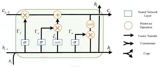
Figure 1.
The structure of long-short term memory (LSTM).
The first step in LSTM is to use the forget gate to decide how much information in is thrown away. The second step is to use update gate to decide how much new information in is added to . Through the above two steps, can be obtained. Finally, by putting through the tanh function and using output gate, we can get the output .
In a translation problem, a sentence is treated as a time series. A word is in the form of a vector, first through a linear layer (embedding layer), and then input to LSTM for subsequent translation. Essentially, the encoder-decoder model is a translation model in image caption, and the model translates an image into a sentence. If the full connection layer extracted from CNN is used as the input of LSTM at −1 time, then the NIC model [9] can be obtained, which is as follows:
where are learning parameters and CNN encodes the image as a vector input to LSTM.
It should be noted that in the NIC model, the information of an image is input only once, and the subsequent process generates sentences only by LSTM. Obviously, this method does not enable the network to make full use of the extracted image information, because the model only “looks” at the image once. In the NIC model, the fully connected layer in CNN is used as image coding. Assuming that the size of the final convolutional layer of the CNN is 7 × 7 × 512, and the fully connected layer is an average pooling of the feature maps, that is, to average the values of 7 × 7 regions on each feature map. Therefore, the NIC model treats these 49 regions equally without any differentiated view, which is different from the way people describe an image.
The attention model has been improved for the NIC model and contains the input of image information at every time step in the decoding process. The encoder extracts the convolution layer of CNN (usually the last convolution layer of the network) rather than the fully connected layer. We also assume that the size of the final convolutional layer of the CNN is 7 × 7 × 512, and the attention model will first learn 7 × 7 weight values, indicating different attentions to different regions. Next, it will perform pooling according to these weight values. Therefore, the attention model treats these 49 regions with different attentions.
The core of the attention model is that when using the extracted convolution layer, the attention model does not necessarily pay attention to all areas of an image, and more likely it is only using the information of some areas of the image. For example, when generating the word “airplane”, the model only needs to focus on the area containing the airplane in the image, instead of observing the entire image. This mechanism is consistent with human visual mechanisms. When a human observes an image, the focus of vision only stays in some areas, not all areas.
Since LSTM inputs additional image information each time, the same changes need to be made to Equations (1)–(4). Taking Equation (1) as an example, its new expression should be as follows:
where is the encoding vector with attention. Its value is determined by the hidden layer of LSTM and the whole image, which can be simply expressed as:
where is an attention function. is the convolution layer extracted by CNN, and k is the size of the feature maps extracted by CNN, which is equal to the height of the feature maps multiplied by the width of the feature maps, and (C is the number of feature maps). According to the difference of , attention mechanisms can be divided into two kinds, one is stochastic “hard” attention, the other is deterministic “soft” attention [10].
Because the implementation of soft attention is relatively simple and is effectively equivalent to hard attention, only soft attention is introduced here. Soft attention learns k weights at each time t, and those weights represent the attention level of k areas in I, which can be expressed as follows:
where is the weight to be learned. and are parameters to be learned. is a matrix with all elements set to 1, which is used to adjust the dimensions of the matrix. Since the sum of k weights is 1, the softmax function is used. It can be seen that in the attention model, the representation of an image is actually a region weighting of I. The model learns k weights at each time t, thus achieving an image representation with attention.
2.2. The Multi-Level Attention Model for Remote Sensing Image Caption
Single attention structure is insufficient to express visual and semantic features. Therefore, we propose a model with three attention structures, which represent the attention to different areas of the image, the attention to different words, and the attention to vision and semantics, as shown in Figure 2.
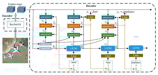
Figure 2.
The architecture of our multi-level attention model. Firstly, and image is resized into 224 pixels × 224 pixels, and then ResNet101 is used as the decoder to extract the convolution layer of the image. In the decoder, h and c are firstly initialized using extracted feature maps and “Transform” blocks. Arrows indicate the flow of data. The “attention1” gets the expression of attention to different regions of the image, which is expressed by the vector . The “attention2” gets the expression of attention to different words in a sentence that has been generated, which is expressed by the vector . The “attention3” refers to the attention to and , which is expressed by the vector . The obtained by attention is combined with the predicted of the previous moment and input into the LSTM at time t. These operations predict the word , and will continue until .
For the attention1 structure, it is similar to the general attention structure in Section 2.1, as shown in Figure 3, but the difference between our attention1 structure and the general attention model lies in the change of the function . The input parameter of changes to . This means that the model first calculates at time t and learns the visual expression according to it.
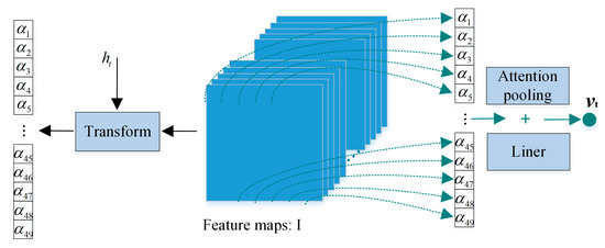
Figure 3.
The architecture of attention1. This structure can learn a set of weights, which represent the degree of attention to different areas of the image.
In the attention2 structure, we mainly consider the guidance of the generated words to the subsequent word generation. This is similar to the language model, but here it is not only to predict the next word according to the vector obtained by attention2, but to select the vector again through attention3. The schematic diagram of attention2 is shown in Figure 4.
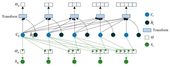
Figure 4.
The architecture of attention2. This structure can learn a set of weights, which represent the degree of attention to different words that have been generated. At each time t, attention2 uses the previously predicted word information.
In attention2, we use in LSTM to represent word information and add information at each moment to learn a set of weights. Then, the weights act on to get the final expression for semantic features, which is expressed by the vector . This process can be expressed by the following equations:
where is the weight used to express attention to words. and are the parameters to be learned. These weights act on to get the expression for the semantic vector.
We achieve the attention representation for different regions of the image by attention1, and the attention representation for different words by attention2. Next, we need to add the attention3 structure. This structure is mainly to consider some fixed sentence expressions, such as “be able to”, that is to say, after “be able” appears, when predicting the next word, the attention to the image can be small. On the contrary, when predicting words like “airplane”, the attention3 would pay more attention to images than words. This attention structure can guide the model to automatically choose whether to focus on image information or focus on sentence structure information when generating a caption as shown in Figure 5.
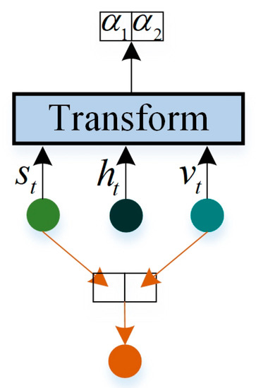
Figure 5.
The architecture of attention3. This structure can learn a set of weights, which reflect the degree of attention to visual and semantic information. and are obtained by attention1 and attention2, respectively.
The structure of attention3 can be expressed by the following equations:
where and are the parameters to be learned. The range of is [0, 1], and . If is 1, it means that the model is completely dependent on the image information, and if its value is 0, it means that the model is completely dependent on the sentence information. obtained by the multi-level attention structure is used to predict the next word at time t.
In fact, the main difference between our model and the NIC model is that our model adds three attention structures. And the equations involved in three attention structures are mainly the way of obtaining attention weights, which is achieved by the combination of liner layers and a softmax function. Assume that the size of the feature map extracted by CNN is 7 × 7 × 512, the hidden state dimension in LSTM is 512, and the number of neurons in the attention network is 256. Taking Equations (10)–(12) as an example, the process of getting attention weights based on these equations can be shown in Figure 6; all three attention structures can be built like this.
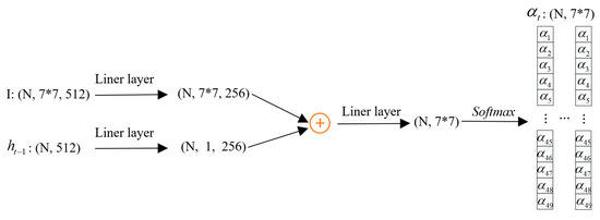
Figure 6.
The process of getting attention weights based on Equations (10)–(12). N is batch size.
As we can see from Figure 6, from only using linear layer and softmax functions, attention structure can be realized. The linear layer is for the transformation of dimensions, and the softmax function is to get attention weights. and in equations are the parameters of the linear layer, which need to be learned. Thanks to the application of the back propagation (BP) algorithm [32], we only need to build a forward network including these three attention structures to learn these parameters.
3. Experiments
In this section, we first introduce the modified datasets and then introduce the implementation details, results and analysis related to our experiments.
3.1. Modified Datasets
In the task of remote sensing image description, the three main data sets are Sydney [1], UCM [1], and RSICD [2]. Here is a brief introduction to these datasets:
- (1).
- The Sydney dataset has only 613 images, each image contains 5 captions, and the dataset has a total of 237 words. The image pixel resolution is 0.5 m. Its caption is more appropriate, but the amount of data is small.
- (2).
- The UCM dataset has 2100 images, each image contains 5 captions, and the dataset has a total of 368 words. The pixel resolution of the image is 0.3048 m. Its caption is relatively simple, and its sentence pattern is rather rigid.
- (3).
- The RSICD dataset has 10,921 images, each image contains 5 captions, and the dataset has a total of 3325 words. The data are collected from Google Earth, Baidu Map, MapABC, Tianditu [2].
Although the contribution of Sydney, UCM and RSICD datasets to the remote sensing image captions is enormous, their shortcomings are also obvious. According to what we have found, the rates of error descriptions in Sydney, UCM, and RSICD datasets are at least 8.62%, 3.56% and 13.12%. Learning the wrong data can only obtain incorrect captions, and the results are meaningless. The main adverse effects of incorrect data are as follows:
- (1).
- For the word “airplane” misspelled into “airplan”, although people can judge the error, it is difficult for a computer to achieve this, because words in the computer are represented in vector form, even “lot” and “lots” are different vectors.
- (2).
- Word frequency refers to the number of times that a word appears in all descriptive sentences. Generally, misspelled words tend to have a very low word frequency. Words with too low of a word frequency are usually abandoned as uncommon words, which is a waste of data.
- (3).
- If words are represented by a well-trained word embedding, then “lot” and “lots” will be very close to each other in the vector space. But for misspelled words, the word embedding either does not exist or does not correspond, which would affect the final result.
Several wrong ways for descriptions are as follows:
- The word is misspelled (no such word), such as “different” misspelled into “differenet”.
- The word is misspelled (spelled into other words), such as “tree” misspelled into “tress”.
- Singular and plural errors, such as “many building” should be “many buildings”.
- Misuse of parts of speech, such as “arranged compact” should be “arranged compactly”.
- Word connection errors, such as “parkinglot” should be “parking lot”.
- Punctuation errors, such as “fense,” should be “fense”.
- Grammatical errors, such as “makes” should be “making” in some cases.
- Redundancy of some spaces and punctuation marks.
- The sentence described is not appropriate.
We count the number of words and sentences modified, and the number of images involved in the modification. Also, we count the percentage of modifications. The results are displayed in Table 1.

Table 1.
The number of modifications for the three datasets. For example, we modify 38 words for the Sydney dataset, and this dataset has a total of 237 words, so the percentage we modified is 38/237 = 16.03%.
In Table 1, if there are multiple errors in a sentence, we count the sentence only once, and if there are multiple wrong sentences in an image, we count the image only once. From Table 1, we can see that every dataset has many errors. By correcting these errors, the quality of these datasets can be improved, which is more conducive to the study of remote sensing image captioning. In fact, the number of modified words and related sentences can better reflect the cleanliness of the modified datasets because the real label of an image is the sentence in the image caption.
To further illustrate the differences between before and after data modification, we have counted the changes in the number of words in different situations. The statistical results are shown in Table 2.
Table 2.
Changes in the number of words before and after modifying the data.
In Table 2, it should be noted that “words in validation dataset” and “words only in validation dataset” are different. “Words only in validation dataset” means that words appear only in the validation dataset, not in the training dataset and the test dataset. Generally, if a word does not exist in the training dataset, it is difficult to generate a caption containing the word in the test dataset because this usually means the distribution of the training dataset is different from that of the test dataset. Therefore, if the number of such words is too large, it will have a negative impact on the results of the caption. The “all words” represents the number of words in the entire dataset, including the training dataset, validation dataset, and test dataset. The number of “all words” affects the one-hot representation of the word. If the number is too large, a larger vector will be needed for the representation of a word, and the space of words will become sparse. However, if the number of “all words” is too small, the description will be very simple and rigid. The “word frequency” has been discussed before. If there are too many words with low word frequency, it will cause a waste of data.
As can be seen from Table 2, all the numbers have decreased after data modification, which indicates that the modified datasets are better and more suitable for research.
In addition to the above modifications, we have also modified other unreasonable parts of the caption file. The caption file is saved according to the COCO dataset style [24], which is as follows:
| {‘dataset’ : ‘Sydney’, |
| ‘images’ : [‘filename’ : ‘1.tif’, |
| ‘raw’:’A residential area with houses arranged neatly.’, |
| ‘sentid’:0, |
| ‘tokens’ : [‘A’, ‘residential’, ‘area’, ‘with’, ‘houses’, ‘arranged’, ‘neatly’] |
| …} |
Generally, ‘raw’ and ‘tokens’ are mainly used when using the caption file. According to our observation, some of them do not correspond to each other. So, we have also repaired this part.
For the existing remote sensing image caption methods, the original data sets UCM, Sydney and RSICD are used. We have said that these unmodified data sets contain a lot of errors, so the results are not credible. But for the sake of explanation, we still designed a comparison experiment between the old and the new data.
3.2. Evaluation Metrics
Since the scoring of image captions is only a comparison between the caption generated by the model and the labels of manual captions, the evaluation metrics chosen in this paper are consistent with the evaluation metrics used in natural image captions. They are BLEU [33], Meteor [34], ROUGE_L [35], CIDEr [36], and SPICE [37]. BLEU includes bleu-1, bleu-2, bleu-3 and bleu-4.
In addition to the quantitative evaluation metrics above, we also explored the issue of sentence diversity in remote sensing image description for the first time. Generation diversity is an important part of image description evaluation. In paper [9], “caption not present in the training set” is used as the discussion index of generation diversity, but that discussion is superficial. In this paper, we will analyze the generation diversity in more detail.
3.3. Training Details
In data preprocessing, we only retain the caption with a length less than 30 words, and because these datasets are not particularly large, we choose to keep all words that appear more than two times. In the LSTM, the hidden size is set to 512 and the embedding or liner size is also 512. CNN uses pretrained resnet101 [26], and the original images are resized into 224 × 224. The size of feature maps extracted by this method is 1024 × 14 × 14. Both the encoder and the decoder have chosen the Adam optimizer.
When training the decoder only, the batch size is set to 32, the learning rate is 10−4, and the maximum epoch is 50. If the loss does not decrease after 2 epochs, the learning rate is multiplied by 0.8. If the loss does not decrease after six epochs, stop training. Then to fine-tune the best results obtained from the above training, the encoder is also trained. In this process, the learning rate of the encoder is set to 5 × 10⁻⁵ and the learning rate of the decoder is set to 10−5. The strategy of epoch and learning rate decay are the same. Note that because the encoder needs to be trained in the fine-tuning stage, there are many parameters and the batch size needs to be reduced appropriately. We set the batch size at the fine-tuning stage to 16. In all experiments, we use a beam size of three in the generation of captions. On the largest dataset RSICD, our model training time is less than eight hours on a single NVIDIA 1080 GPU.
3.4. Experimental Results
3.4.1. Quantitative Comparison of Different Methods
Firstly, we quantitatively verify the performance of our model. We design experiments on the unmodified dataset and modified dataset. The best results in paper [1] and paper [2], as well as the general attention model are compared. In Table 3, Table 4 and Table 5, “-“ indicates that the metric is not used and the bold font indicates the best result. Att1 means that only attention1 is used. Att1 + att3 indicates that attention1 and attention3 structures are used. And b1, b2, b3, b4, M, R, C and S represent bleu-1, bleu-2, bleu-3, bleu-4, Meter, ROUGE_l, CIDEr and SPICE, respectively.
Table 3.
The comparison of different methods on the unmodified and modified datasets of Sydney. The bold value is the highest score.
Table 4.
The comparison of different methods on the unmodified and modified datasets of UCM. The bold value is the highest score.
Table 5.
The comparison of different methods on the unmodified and modified datasets of RSICD. The bold value is the highest score.
From the three tables, we can see that our models perform better on all three datasets. And “att1 + att3” indicates that only attention1 structure and attention3 structure are used Compared with the general attention model (att1) and “att1 + att3” model, our model can express sentence information better, which means that our model with multiple attention structures has a better performance than the model with simple attention structures. Even on the unmodified data, our model can also achieve the best results under almost all the evaluation metrics.
Because the selection of image information is added, the effect of att1 + att3 is better than that of att1. Further, adding attention to the semantic information makes the result of our model better. Furthermore, almost all models perform better on modified datasets than on unmodified datasets. This is due to the powerful expressive ability of LSTM. When the dataset is correct, LSTM can learn better expression, so it has better performance on modified datasets. However, when there are many errors in datasets, it is easy to learn some error information about the dataset, which leads to the general performance on the unmodified dataset.
3.4.2. Comparison of Unmodified Datasets and Modified Datasets
In order to further verify the difference in the effect of the model before and after data modification. We calculated the ratio of increased scores for each model after the data correction, and thus obtained Figure 7.
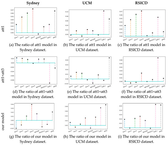
Figure 7.
The ratio of model scores increased after datasets were modified. The figure is the result of three models on three datasets, so there are nine sub-figures. Each sub-figure has eight evaluation metrics on the x-axis, and the y-axis value is the ratio, which equals to: (score on modified dataset–score on unmodified dataset) / (score on unmodified dataset). The upward point means that the model scores higher on the modified dataset than the unmodified dataset.
As can be seen from Figure 7, due to the correction of the descriptions, in most cases, the scores of a model have increased on the modified datasets, and the maximum increase is about 7%. This result mainly comes from the reduction of error data in the modified datasets. We have introduced the data repair work in Section 3.1. Taking RSICD as an example, the proportion of sentences repaired is 13.12%. The modified datasets make the model easier to learn, and the correct label makes the scores more reasonable. In addition, it can be observed in Figure 7 that the score increase is not obvious on the Sydney dataset. This is because Sydney is a small dataset with only 613 images and 217 words. Under such data volume, it is difficult to measure the effect of a deep learning model. Moreover, a few repairs of the Sydney dataset cannot achieve an obvious increase in scores.
We let our model train on the unmodified and modified datasets. On the unmodified dataset, the model generates some wrong captions, while for the same images, the correct captions can be generated if the model is trained on the modified dataset; Figure 8 shows examples of how the modified datasets can effectively avoid the model learning the wrong captions. This is mainly due to the correction of errors in the datasets.
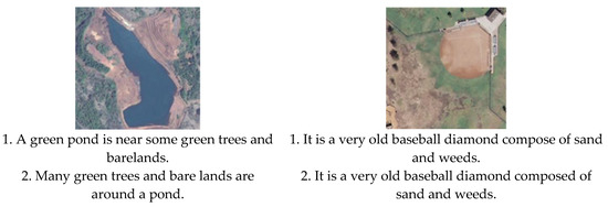
Figure 8.
The captions generated by our model after training on the unmodified and modified datasets. The sentence 1 uses the unmodified datasets, and the sentence 2 uses the modified datasets. Underlined words represent where the caption is wrong.
3.4.3. Comparison of Generation Diversity
We also explored the relationship between generation diversity and scores of a model. Generation diversity is an important part of image description evaluation. In paper [9], “caption not present in the training set” is used as the discussion index of generation diversity.
The higher the proportion of generated descriptions by a model in the training set, the lower the generation diversity of the model. It should be noted that it is meaningful to evaluate the diversity of models only when they have similar scores, because if the scores are very low, even if the models have high diversity, the generated descriptions by these models are only wrong. We calculated the proportion of generated descriptions in the training dataset for three models, and we formed Table 6.
Table 6.
The proportion of generated descriptions not in the training dataset of each model. The bold value is the lowest proportion.
From Table 6, we can see that our model not only guarantees the highest scores but also guarantees the diversity of generated sentences. For all datasets, our model achieves four best results. What does the “proportion” exactly mean? If the proportion is too small, it means that the model has not learned the sentence expression of the training dataset. If the proportion is too large, the model cannot generate sentences outside the training dataset, then the semantic diversity of the model is low. A model, after receiving enough training, is more inclined to use the existing sentences of the training dataset as the generated description, because it is easier to use the “example” directly. This is not in line with the expression of intelligence, because human language is extremely rich, the same scene can be expressed in a variety of different sentences. Therefore, when designing a model, the proportion should be lowered as much as possible without decreasing its score, so that the model can generate more sentences that do not exist in the training dataset.
Some sentences generated by our model not present in the training dataset are shown in Figure 9. It can be seen that the new sentences are learned by our model and the images are described appropriately.
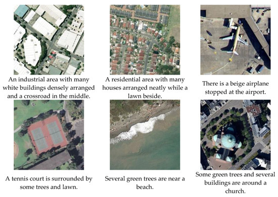
Figure 9.
Generated sentences not present in the training dataset.
4. Discussion
4.1. Effectiveness of Attention Structure
In order to verify the effectiveness of attention structure, we change the attention2 structure to the normal liner layer, that is, we do not learn attention weights, and treat all words equally. In addition, we used different numbers of words to predict the next word and formed Table 7.
Table 7.
Performance of our model under different numbers of words. The bold value is the highest score.
Comparing Table 7 with Table 3, Table 4 and Table 5, we can see that our multi-level attention model has the best performance. This is because our attention2 structure has different attention for different words. In Table 7, as the number of words increases, the performance of the model roughly begins to decline. Especially when the number of words is four, the scores are reduced. This is mainly due to the reason that even if all words are used, they cannot be fully utilized because the model treats all words equally. If we use too many words, useless words will only bring a lot of noise and have a negative impact on the model, which leads to a decline in performance. Therefore, the attention structure is effective, which can automatically learn how to observe things with a focus just like humans.
4.2. Effectiveness of Our Multi-Level Attention Model that Mimics Humans for Image Caption
In Section 4.1, we can see the effectiveness of the attention mechanism, which is one of the reasons why our model works well. However, the attention structure cannot be added to a model at will, and how to adapt attention to image tasks is also the focus of research. At this point, we mainly refer to the thinking process of human beings when describing an image. In order to verify the effectiveness of this point, we visualize our multi-level attention structure when generating a caption of an image, and two examples are obtained as Figure 10 and Figure 11.
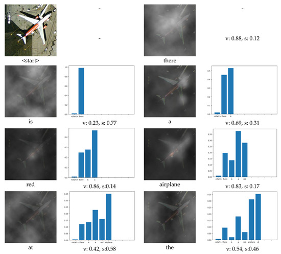
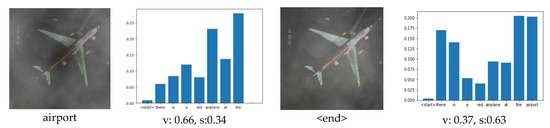
Figure 10.
Visualization of our multi-level attention structure when generating the description: “there is a red airplane at the airport”. The figure above each word indicates the attention to the image, which is the visualization of the attention1 structure. The brighter the area on the figure, the greater the attention to that area. The blue bar graph indicates attention to the past words when generating the current word, which is the visualization of the attention2 structure. “v” means “visual”, and “s” means “semantic”. “v: 0.37, s:0.63” means that 37% of attention is visual and 63% of attention is semantic, which is the visualization of the attention3 structure.
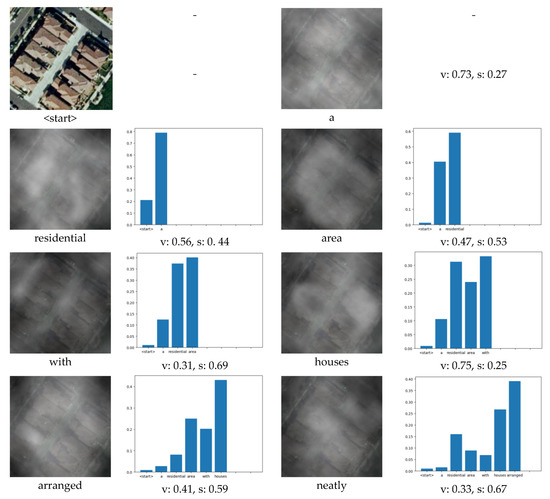
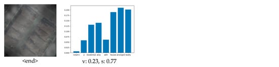
Figure 11.
Visualization of our multi-level attention structures when generating the description: “a residential area with houses arranged neatly”. The figure above each word indicates attention to the image, which is the visualization of the attention1 structure. And the brighter the area on the figure, the greater the attention to that area. The blue bar graph indicates attention to the past words when generating the current word, which is the visualization of the attention2 structure. “v” means “visual”, and “s” means “semantic”. “v: 0.23, s: 0.77” means that 23% of attention is visual and 77% of attention is semantic, which is the visualization of the attention3 structure.
When generating some objects that can be directly observed in the image, the attention1 structure will focus on the area containing the object in the image. For example, in Figure 10, when generating the word “airplane”, the attention1 structure mainly focuses on the area containing the airplane in the image, and at this time, v = 0.83, that is, the attention3 structure will pay attention to the visual information generated by the attention1. When generating the words “houses” and “area” in Figure 11, the attention1 structure is mainly focused on the area containing houses on the image. At the same time, the attention3 structure will pay attention to the visual information generated by attention1. When generating some words that are not nouns, such as “the” or “is”, there is no region corresponding to these words in the image. Therefore, at this time, the attention1 structure is invalid. Due to our multi-level attention model adding the attention2 and attention3 structures, it can automatically pay more attention to the semantic information and can still generate the correct words when the attention1 structure is invalid. For example, in Figure 10, when generating the word “is”, s = 0.77, that is to say, 77% of the attention is on the semantic information. Additionally, observing the visualization of the attention2 structure, we can see that the generation of “is” mainly depends on the word: “there”, which is obviously in line with common sense, because “there is…” is a common sentence collocation. In Figure 11, when generating the word: “with”, s = 0.69, that is to say, most of the attention is paid to semantic information, while little attention is paid to image content. Moreover, from the blue bar chart in Figure 10 and Figure 11, it can be seen that there is little attention paid to the initial word “< start >“ when generating words. The current word mainly depends on several nearby words, which is also consistent with our daily expression semantics, that is, in a sentence, a word has a greater relationship with the adjacent words.
According to the above analysis, it can be seen that our method is effective in remote sensing image description tasks. This is mainly due to the fact that our method is a closer imitation of attention mechanism of human beings. The research of image description tasks cannot be separated from the extraction of image information and sentence information. The extraction of information in human life is efficient, and this kind of extraction is active, that is, people only pay attention to the useful information, but ignore the useless information. Our method is a closer imitation of this mechanism of human beings. We are not only imitating an “unequal” attention mechanism, but the thinking process of humans when describing an image. This requires attention to the images, sentences, and between vision and semantics. Therefore, the performance of our method is significantly improved.
5. Conclusions
In this paper, we do a lot of modification works on the existing remote sensing image caption datasets and make the modified datasets public. The original datasets come from [1,2], but there are a lot of errors in these original datasets, which cause the model to learn incorrect descriptions. By training with the modified datasets, the results are more reliable.
Inspired by the attention mechanism widely used in image tasks, we propose a multi-level attention model. Our model contains three effective attention structures. The first attention structure mainly focuses on the image, which is used to simulate people’s observation behavior of an image. At a certain time, it focuses on only some but not all areas in the image. The second attention structure is focused on semantic information, which is similar to people’s attention to language. The form of the next word in a sentence is related to some words that have appeared before. The third attention structure is a re-selection of vision and semantics, which is similar to that when people describe an image. Sometimes, it is necessary to focus on the image, and sometimes it is not necessary to focus on the image. In order to verify the validity of our model, we conducted a lot of comparative experiments, which confirmed that the multi-level attention model is effective and achieved state-of-the-art results. We also quantitatively analyzed the diversity of the model. The model achieved good diversity and was able to generate some sentences that did not exist in the training set.
We hope that the work of this article can be helpful for remote sensing image caption tasks and we also hope that our models can be applied in other fields.
Author Contributions
Methodology, S.F.; Experimental results analysis, S.F. and Y.L.; Oversight and suggestions, Y.L. and L.J.; Writing—review and editing, Y.L. and S.F.; Investigation, S.F., Y.L., R.L. and R.S.; Funding acquisition, Y.L. All authors have read and agreed to the published version of the manuscript.
Funding
This work was supported in part by the National Natural Science Foundation of China under Grants 61772399, U1701267, 61773304, 61672405, and 61772400, in part by the Key Research and Development Program in Shaanxi Province of China under Grant 2019ZDLGY09-05, in part by the Program for Cheung Kong Scholars and Innovative Research Team in University under Grant IRT_15R53, and in part by the Technology Foundation for Selected Overseas Chinese Scholar in Shaanxi under Grants 2017021 and 2018021.
Acknowledgments
The author would like to show their gratitude to the editors and the anonymous reviewers for their insightful comments.
Conflicts of Interest
The authors declare no conflict of interest.
References
- Qu, B.; Li, X.; Tao, D. Deep semantic understanding of high resolution remote sensing image. In Proceedings of the International Conference on Computer, Information and Telecommunication Systems (CITS), Kunming, China, 6–8 July 2016. [Google Scholar]
- Lu, X.; Wang, B.; Zheng, X. Exploring Models and Data for Remote Sensing Image Caption Generation. IEEE Trans. Geosci. Remote Sens. 2017, 56, 2183–2195. [Google Scholar] [CrossRef]
- Romero, A.; Gatta, C.; Camps-Valls, G. Unsupervised Deep Feature Extraction for Remote Sensing Image Classification. IEEE Trans. Geosci. Remote Sens. 2016, 54, 1349–1362. [Google Scholar] [CrossRef]
- Lu, X.; Zheng, X.; Yuan, Y. Remote Sensing Scene Classification by Unsupervised Representation Learning. IEEE Trans. Geosci. Remote Sens. 2017, 55, 5148–5157. [Google Scholar] [CrossRef]
- Gong, C.; Yang, C.; Yao, X. When Deep Learning Meets Metric Learning: Remote Sensing Image Scene Classification via Learning Discriminative CNNs. IEEE Trans. Geosci. Remote Sens. 2018, 56, 2811–2821. [Google Scholar] [CrossRef]
- Baumgartner, J.; Gimenez, J.; Scavuzzo, M. A New Approach to Segmentation of Multispectral Remote Sensing Images Based on MRF. IEEE Trans. Geosci. Remote Sens. 2015, 12, 1720–1724. [Google Scholar] [CrossRef]
- Chang, C.L.; Chiang, S.R.; Ren, H. Real-time processing algorithms for target detection and classification in hyperspectral imagery. IEEE Trans. Geosci. Remote Sens. 2001, 39, 760–768. [Google Scholar] [CrossRef]
- Zhang, L.; Zhang, L.; Tao, D. Hyperspectral Remote Sensing Image Subpixel Target Detection Based on Supervised Metric Learning. IEEE Trans. Geosci. Remote Sens. 2014, 52, 4955–4965. [Google Scholar] [CrossRef]
- Vinyals, O.; Toshev, A.; Bengio, S. Show and tell: A neural image caption generator. In Proceedings of the IEEE Conference on Computer Vision and Pattern Recognition, Boston, MA, USA, 7–12 June 2015. [Google Scholar]
- Xu, K.; Ba, J.; Kiros, R. Show, Attend and Tell: Neural Image Caption Generation with Visual Attention. In Proceedings of the International Conference on Machine Learning, Lille, France, 6–11 July 2015; pp. 2048–2057. [Google Scholar]
- Lu, J.; Xiong, C.; Parikh, D. Knowing When to Look: Adaptive Attention via a Visual Sentinel for Image Captioning. In Proceedings of the IEEE Conference on Computer Vision and Pattern Recognition, Honolulu, HI, USA, 21–26 July 2017. [Google Scholar]
- Shi, Z.; Zou, Z. Can a Machine Generate Humanlike Language Descriptions for a Remote Sensing Image? IEEE Trans. Geosci. Remote Sens. 2017, 55, 3623–3634. [Google Scholar] [CrossRef]
- Karpathy, A.; Fei-Fei, L. Deep Visual-Semantic Alignments for Generating Image Descriptions. IEEE Trans. Pattern Anal. Mach. Intell. 2014, 39, 664–676. [Google Scholar] [CrossRef] [PubMed]
- Wu, Z.; Cohen, R. Encode, Review, and Decode: Reviewer Module for Caption Generation. Available online: https://www.researchgate.net/publication/303521432_Encode_Review_and_Decode_Reviewer_Module_for_Caption_Generation (accessed on 9 March 2020).
- Sadeghi, M.A.; Sadeghi, M.A.; Sadeghi, M.A. Every picture tells a story: Generating sentences from images. In Proceedings of the European Conference on Computer Vision, Crete, Greece, 5–11 September 2010. [Google Scholar]
- Gupta, A.; Mannem, P. From Image Annotation to Image Description. In Proceedings of the International Conference on Neural Information Processing, Doha, Qatar, 12–15 November 2012. [Google Scholar]
- Kulkarni, G.; Premraj, V.; Dhar, S. Baby Talk: Understanding and Generating Simple Image Descriptions. In Proceedings of the Computer Vision and Pattern Recognition (CVPR), Colorado Springs, CO, USA, 20–25 June 2011. [Google Scholar]
- Donahue, J.; Anne Hendricks, L.; Guadarrama, S. Long-term recurrent convolutional networks for visual recognition and description. In Proceedings of the IEEE Conference on Computer Vision and Pattern Recognition, Boston, MA, USA, 7–12 June 2015. [Google Scholar]
- Mao, J.; Xu, W.; Yang, Y. Deep Captioning with Multimodal Recurrent Neural Networks (M-Rnn). Available online: https://arxiv.org/abs/1412.6632 (accessed on 9 March 2020).
- Kinghorn, P.; Zhang, L.; Shao, L. A region-based image caption generator with refined descriptions. Neurocomputing 2018, 272, 416–424. [Google Scholar] [CrossRef]
- Anderson, P.; He, X.; Buehler, C. Bottom-up and top-down attention for image captioning and visual question answering. In Proceedings of the IEEE Conference on Computer Vision and Pattern Recognition, Salt Lake City, UT, USA, 18–23 June 2018. [Google Scholar]
- Lu, J.; Yang, J.; Batra, D. Neural baby talk. In Proceedings of the IEEE Conference on Computer Vision and Pattern Recognition, Salt Lake City, UT, USA, 18–23 June 2018. [Google Scholar]
- Lillesand, T.; Kiefer, R.W.; Chipman, J. Remote Sensing and Image Interpretation; John Wiley & Sons: Hoboken, NJ, USA, 2015. [Google Scholar]
- Vinyals, O.; Toshev, A.; Bengio, S. Show and Tell: Lessons learned from the 2015 MSCOCO Image Captioning Challenge. IEEE Trans. Pattern Anal. Mach. Intell. 2016, 39, 652–663. [Google Scholar] [CrossRef] [PubMed]
- Simonyan, K.; Zisserman, A. Very Deep Convolutional Networks for Large-Scale Image Recognition. Available online: https://arxiv.org/abs/1409.1556 (accessed on 9 March 2020).
- He, K.; Zhang, X.; Ren, S. Deep residual learning for image recognition. In Proceedings of the IEEE Conference on Computer Vision and Pattern Recognition, Las Vegas, NV, USA, 26 June–1 July 2016. [Google Scholar]
- Cho, K.; Van Merriënboer, B.; Gulcehre, C. Learning Phrase Representations Using RNN Encoder-Decoder for Statistical Machine Translation. Available online: https://arxiv.org/abs/1406.1078 (accessed on 9 March 2020).
- Hochreiter, S.; Schmidhuber, J. Long short-term memory. Neural Comput. 1997, 9, 1735–1780. [Google Scholar] [CrossRef] [PubMed]
- Bai, S.; An, S. A survey on automatic image caption generation. Neurocomputing 2018, 311, 291–304. [Google Scholar] [CrossRef]
- Hossain, M.D.Z.; Sohel, F.; Shiratuddin, M.F. A comprehensive survey of deep learning for image captioning. ACM Comput. Surv. 2019, 51, 1–36. [Google Scholar] [CrossRef]
- Kinghorn, P.; Zhang, L.; Shao, L. A hierarchical and regional deep learning architecture for image description generation. Pattern Recognit. Lett. 2019, 119, 77–85. [Google Scholar] [CrossRef]
- Rumelhart, D.E.; Hinton, G.E.; Williams, R.J. Learning Internal Representations by Error Propagation. Available online: https://web.stanford.edu/class/psych209a/ReadingsByDate/02_06/PDPVolIChapter8.pdf (accessed on 9 March 2020).
- Papineni, K.; Roukos, S.; Ward, T. BLEU: A method for automatic evaluation of machine translation. In Proceedings of the 40th Annual Meeting on Association for Computational Linguistics, Philadelphia, PA, USA, 7–12 July 2002. [Google Scholar]
- Denkowski, M.; Lavie, A. Meteor universal: Language specific translation evaluation for any target language. In Proceedings of the Ninth Workshop on Statistical Machine Translation, Baltimore, MD, USA, 26–27 June 2014. [Google Scholar]
- Lin C, Y. ROUGE: A Package for Automatic Evaluation of summaries. In Proceedings of the Workshop on Text Summarization Branches Out (WAS 2004), Barcelona, Spain, 25–26 July 2004. [Google Scholar]
- Vedantam, R.; Lawrence Zitnick, C.; Parikh, D. Cider: Consensus-based image description evaluation. In Proceedings of the IEEE Conference on Computer Vision and Pattern Recognition, Boston, MA, USA, 7–12 June 2015. [Google Scholar]
- Anderson, P.; Fernando, B.; Johnson, M. Spice: Semantic propositional image caption evaluation. In Proceedings of the European Conference on Computer Vision, Amsterdam, The Netherlands, 8–16 October 2016. [Google Scholar]
© 2020 by the authors. Licensee MDPI, Basel, Switzerland. This article is an open access article distributed under the terms and conditions of the Creative Commons Attribution (CC BY) license (http://creativecommons.org/licenses/by/4.0/).