1. Introduction
Satellite-based synthetic aperture radar (SAR) has great potential for flood detection in every weather condition [
1,
2,
3]. A wide-swath SAR satellite, Sentinel-1, contributes toward establishing a systematic early warning system followed by providing damage assessments [
4,
5,
6,
7,
8], whereas high-resolution SAR satellites (e.g., TerraSAR-X/TanDEM-X [
9,
10,
11], Cosmo-SkyMed [
12,
13], and Advanced Land Observation Satellite 2 (ALOS-2) [
14]) provide detailed spatial awareness of the affected area under complicated land-use settings. In particular, L-band SAR has great advantages regarding vegetation penetration and soil moisture measurement for observing the wetlands, for example, in Dabrowska-Zielinska et al. [
15]. In the near future, numerous SAR satellites operated as constellations will enable the near-real-time monitoring of temporal sequences of flood expansion and shrinking.
Various studies have been performed to increase the accuracy of flood detection [
16,
17,
18,
19]. Multiple sensors combine to provide external data [
20,
21,
22,
23], the stacking of pre-flood observations [
24,
25], and applying machine learning, which are the typical methods used for increasing flood detection accuracies [
26,
27,
28]. Furthermore, advanced segmentation schemes have been proposed [
29,
30], as well as the use of polarimetry [
31]. A comprehensive investigation among multiple microwave frequencies has been reported [
32]. Major SAR sources have been closely examined as part of a coherence analysis, which found that coherence analysis is appropriate for inundation detection in urbanized areas. The latest proposals have confirmed these findings through comparison among numerous statistical and/or machine learning methods, which could achieve a 90% overall accuracy [
33,
34]. Nowadays, the development of fully automatic systems has become an achievable goal [
35,
36].
However, state-of-the-art complex methods face some difficulties when they are applied in real crisis response operations. A newly propose42d method applied to a case study resulted in higher accuracy values but does not guarantee the same detection accuracy in other land cover settings. A basic observation scenario using a greater number of observation modes contains more temporal intervals for use in each mode. Flood detection accuracy calculated using those remarkably limited conditions would be easily affected by inter-annual and seasonal land-use changes. In a worst-case scenario, it may be the first acquisition for the satellite observing the area.
Can we not use pre-flood data from different observation modes and different orbits from post-flood observations without decreasing the detection accuracy? In this paper, we report multiple experimental results obtained by applying the existing methods using amplitude and interferometric coherence to such non-uniform observational settings. In early October 2019, typhoon Hagibis hit eastern Japan, causing dozens of floods [
37]. The Japan Aerospace Exploration Agency (JAXA) observed the possible affected areas using its L-band SAR satellite ALOS-2. One emergency observation was carried out on the Nagano Prefecture in Stripmap mode, where scanning using ScanSAR mode was the only pre-flood data from the same orbit. The affected area was mainly observed using Stripmap mode from the neighboring orbit. We closely analyzed the data by comparing the intensity image and the Stripmap–ScanSAR interferometric coherence. We evaluated the detection accuracy and discuss the resulting feasibility analysis in the following sections.
2. Typhoon Hagibis and the Acquired Data
Typhoon Hagibis hit Japan on 12 October 2019 and dozens of rivers were flooded by its heavy rainfall [
37]. Urgent observations using ALOS-2 were carried out to be aware of the possible affected areas. A part of the riverbank of the Chikuma River in the Nagano Prefecture was breached such that rice paddies, crops fields, orchards, and urban regions were flooded. ALOS-2 observed the affected area on 13 October 2019 with its descending orbit (i.e., 11:57 Japan Standard Time, path 20) using the 3-m resolution Stripmap mode. Approximately one hour earlier, the Geospatial Information Authority of Japan (GSI) carried out an aerial optical observation to provide an inundation map [
38]. The inundation map highlights hazard-induced open water surfaces and does not contain potential water surfaces (known rivers, ponds, etc.). Therefore, the GSI-derived map provides an appropriate reference spatial distribution of the inundation area taken just before the ALOS-2 observation.
There had been no previous observation with the Stripmap mode but there had been two ScanSAR observations from the same orbit, whereas three Stripmap observations from a neighboring orbit, namely path 19, had been carried out (
Table 1). The regular Stripmap observation along path 19 aiming at this site has a higher incidence angle than the post-flood observation. Thus, the urgent post-flood observation from path 20 was optimized for visual identification of the flood area, whereas the mismatching of the incidence angle or observation mode caused uncertainty in the detection accuracy when automated methods were used.
We examined the influences of those mismatched pre-and-post data combinations using the data listed in
Table 1. Note that all SAR intensity-based analyses were performed with JAXA’s Level 2.1 standard products, while interferometric analyses were performed with that of Level 1.1 data. JAXA’s operational processor uses the Shuttle Radar Topography Mission 3 (SRTM-3) data for geocoding, and thus, we used the same dataset in this study [
39].
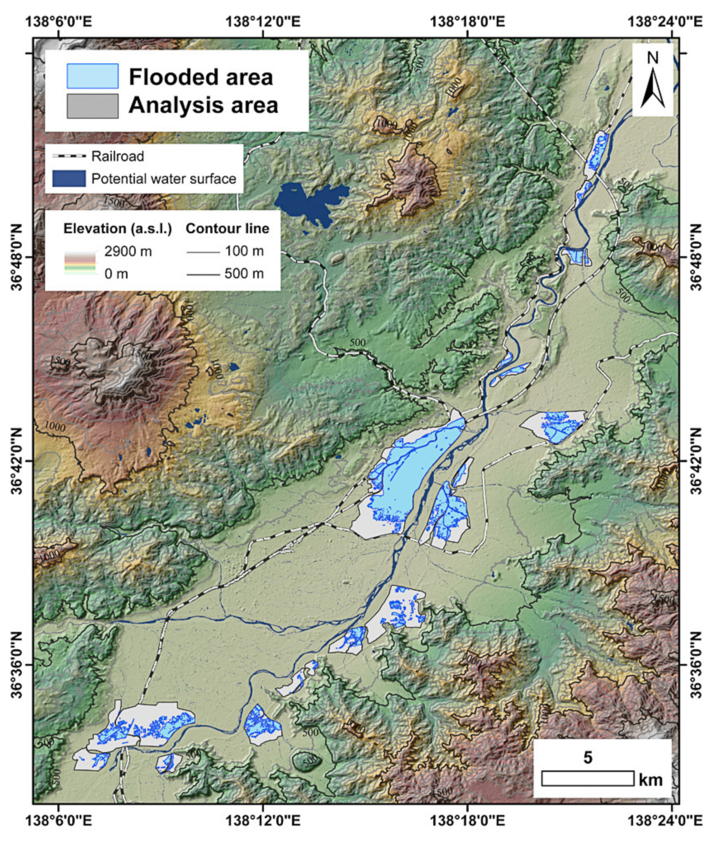
Based on GSI’s reference results, we set the analysis areas such that they surrounded the actual flooded regions, as shown in
Figure 1. The sizes of the flooded and non-flooded areas were 19.05 km
2 and 26.44 km
2, respectively.
3. Analysis Methods
3.1. Intensity Analysis
We applied and compared both a single intensity image and multi-temporal intensity change to detect the open water area on 13 October. The procedure was as follows.
First, we converted the linear value of the SAR intensity image to a logarithmic scale and applied averaging filter with a 10-pixel Manhattan distance diameter. The threshold values for the open water were set to −12 dB for the post-event image and −15 dB for the pre-event images. We made binary images with those values. Finally, we segmented the image with a majority filter using a diameter of 15 pixels. The segmented regions whose size was smaller than 2000 m2 were excluded from the evaluation. We applied the above method for the 29 September 2015 data from path 19 and the 13 October 2019 data from path 20. By comparing the pre- and post-event images in the same season, we could exclude the permanent open water.
3.2. Interferometric Coherence Analysis
Interferometric coherence is the correlation of the complex amplitude between the two observations, namely the “master” and “slave.” The interferometric coherence γ is calculated using:
where
M and
S are the samples of the master and slave single-look complex (SLC) images, respectively. “*” denotes the multiplication. The bar above them denotes the complex conjugate and the brackets represent the ensemble average. In short, the coherence
γ represents the uniformness of the interferometric phase, which strongly depends on the stability of the scatterers. Thus,
γ is high as long as the dominant scatterer is identical between two observations, while it decreases when the scatterers are non-identical. In general,
γ is high for an urban area, while it is low for an unstable and/or smooth surface, such as water, vegetation, and road. The relationship between the coherence and vegetation is a function of the temporal baseline of the interferometric pair, which for farmland in particular, depends on the farming schedule.
In the context of disaster monitoring, an interferometric coherence decrease is used for damage detection. That is, the decrease of the coherence represents the change of dominant scatterers, including the temporal decorrelation. This is called a multi-temporal interferometric coherence change detection. The decrease in coherence
dγ is calculated using the pre-event coherence
γpre and the co-event coherence
γco, as shown in Equation (2):
This value is used mainly for flood detection in urban areas. For vegetated surfaces, due to the naturally low coherence, dγ is small and not reliable. In addition, the height of the dominant scatterer should be considered for flood detection. If the scatterers are not on the ground (e.g., the roof of a building), they do not decrease the coherence of the flood data.
In this paper, we applied an averaging filter with a window size of 8 × 3 in the range and azimuth direction, respectively, for a ScanSAR-based interferogram to reduce the ambiguous signals of ScanSAR. Next, we calculated the coherence value with a 5 × 5 moving window and extracted the flooded area with a threshold of
dγ = 0.3. These values were experimentally derived from preceding research [
26,
40,
41]. Finally, we applied an iterative median filter with a 5 × 5 window for segmentation and acquired an inundation map.
We applied the method above for the 12 March 2019 to 27 August 2019 data pair from path 19 and the 14 April 2019 to 29 September 2019 data pair from path 20 as a pre-event dataset while the 29 September 2019 to 13 October 2019 data pair from path 20 was used for the co-event dataset. Note that the datasets from path 20 were ScanSAR–ScanSAR or ScanSAR–Stripmap interferograms, and thus, had a worse resolution than the path 19 dataset.
4. Results
We evaluated the flood detection results using overall accuracy (OA) and its Cohen’s kappa coefficient (K), as well as the critical success index (CSI).
OA is calculated using:
where
T,
F,
P, and
N denote true, false, positive, and negative, respectively.
K represents the reliability of the results and is calculated using:
where
Pe represents the probability of a random agreement and is found using:
CSI is the statistical value that removes the
TN value from
OA to evaluate the detection accuracy when the
TN value becomes larger than the others:
As the GSI ground truth data excluded the known permanent water, such as ponds and rivers, the scores for the intensity-based methods were almost the same. Their producer’s accuracy was quite low, probably due to the shallow water. The effects of the buildings in the urban area and the crops in the farmland were large. Coherence-based analyses obtained higher scores (approximately 70% for OA in both path 19–path 20 and path 20–path 20 cases); however, K and CSI remained low because the producer’s accuracy was no more than 40%.
On the other hand, the combination of both multi-temporal intensity and coherence methods increased the score for the user’s accuracy. Once we could combine both the intensity and coherence of both path 19 and path 20, the producer’s accuracy and OA increased to 62% and 78%, respectively, with a K of 0.54. This value is acceptable compared with other existing methods. For all combinations, the user’s accuracy remained above 80%. In short, if we could merge the results using ScanSAR or neighboring orbit(s), the detection accuracy became compatible with that of ideal conditions. Further discussion is described in the next section.
5. Discussions
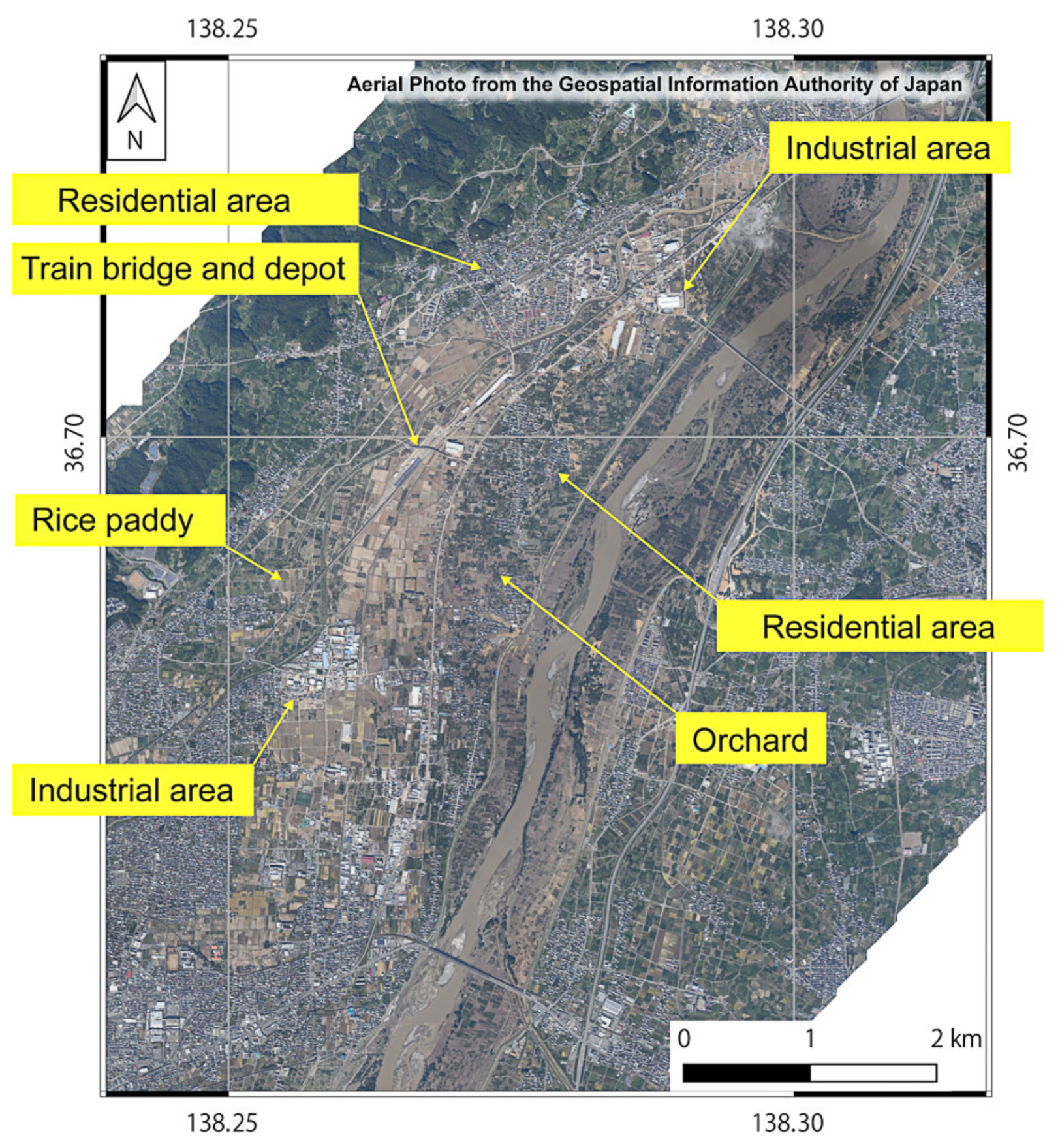
To further investigate the detection results, we focused on the data from Nagano and Nakano city, the largest flooded area in the middle of
Figure 1.
Figure 3 shows an optical image of the close-up area. As shown in the image, croplands and orchards are dominant in the middle of the region. A train bridge crossing is located there, along with a neighboring depot. The northern and southern parts are industrial and residential areas.
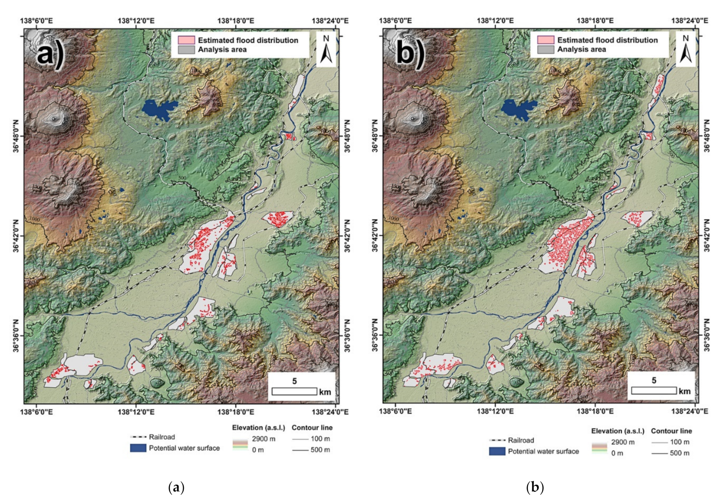
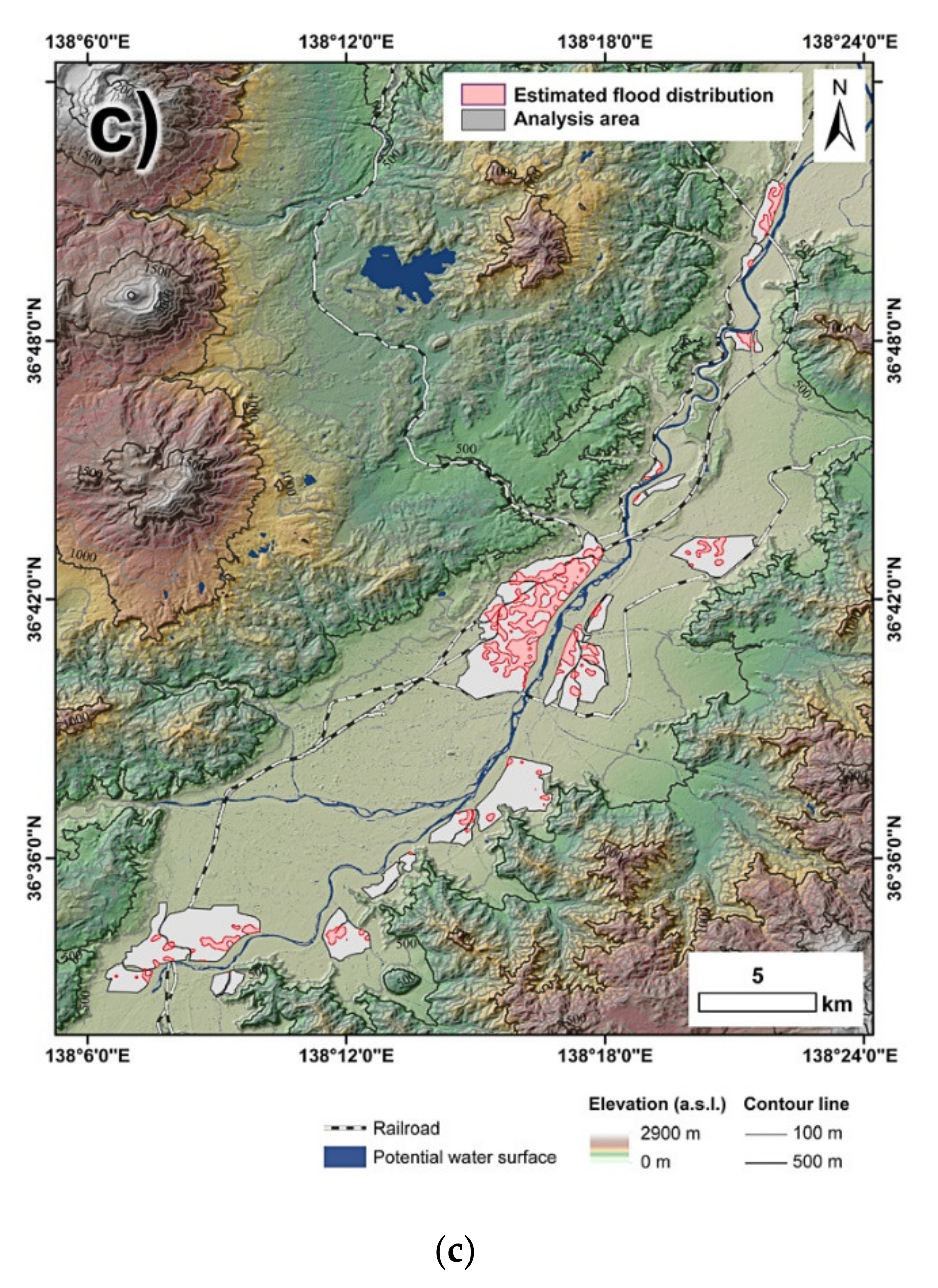
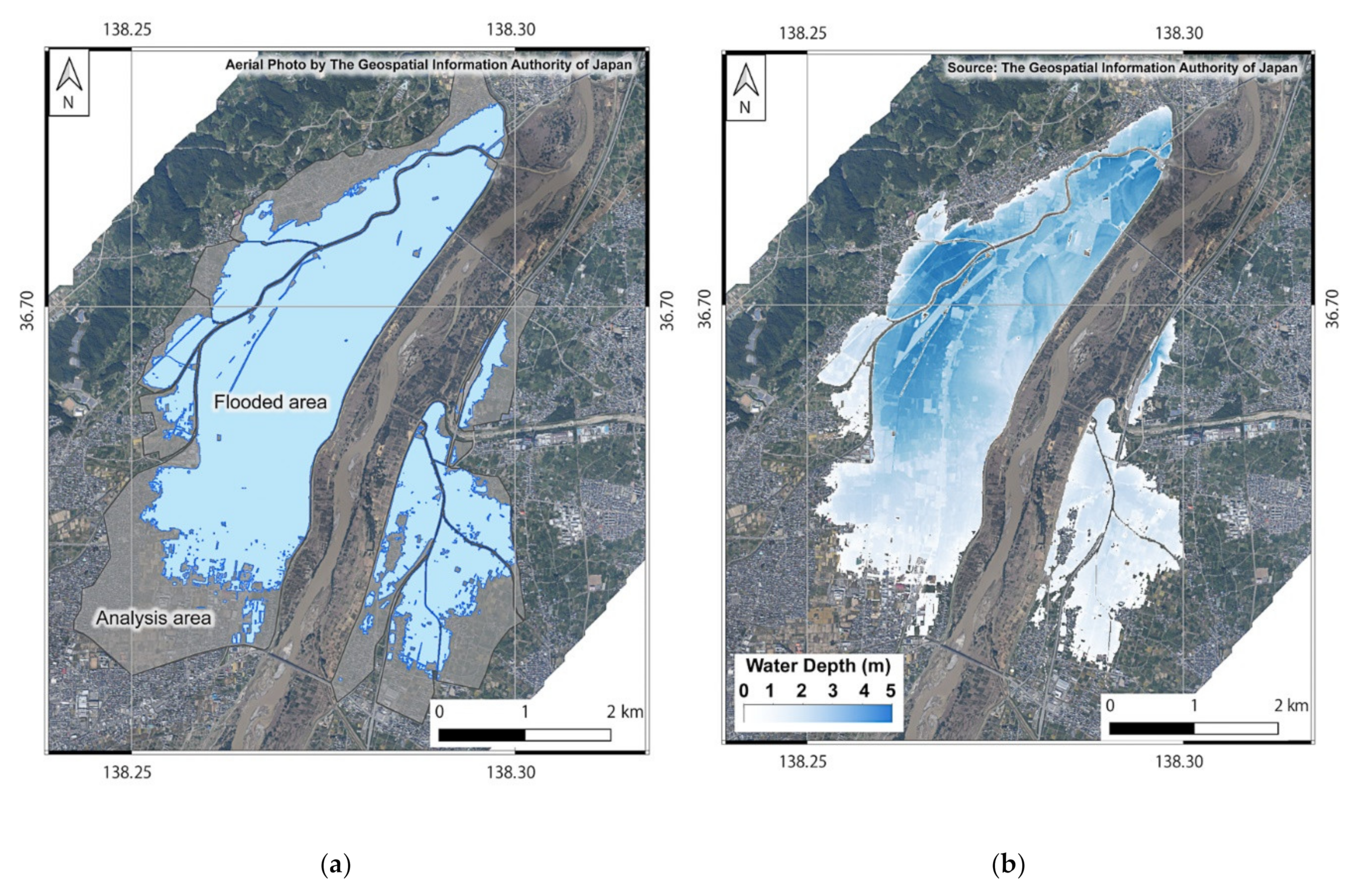
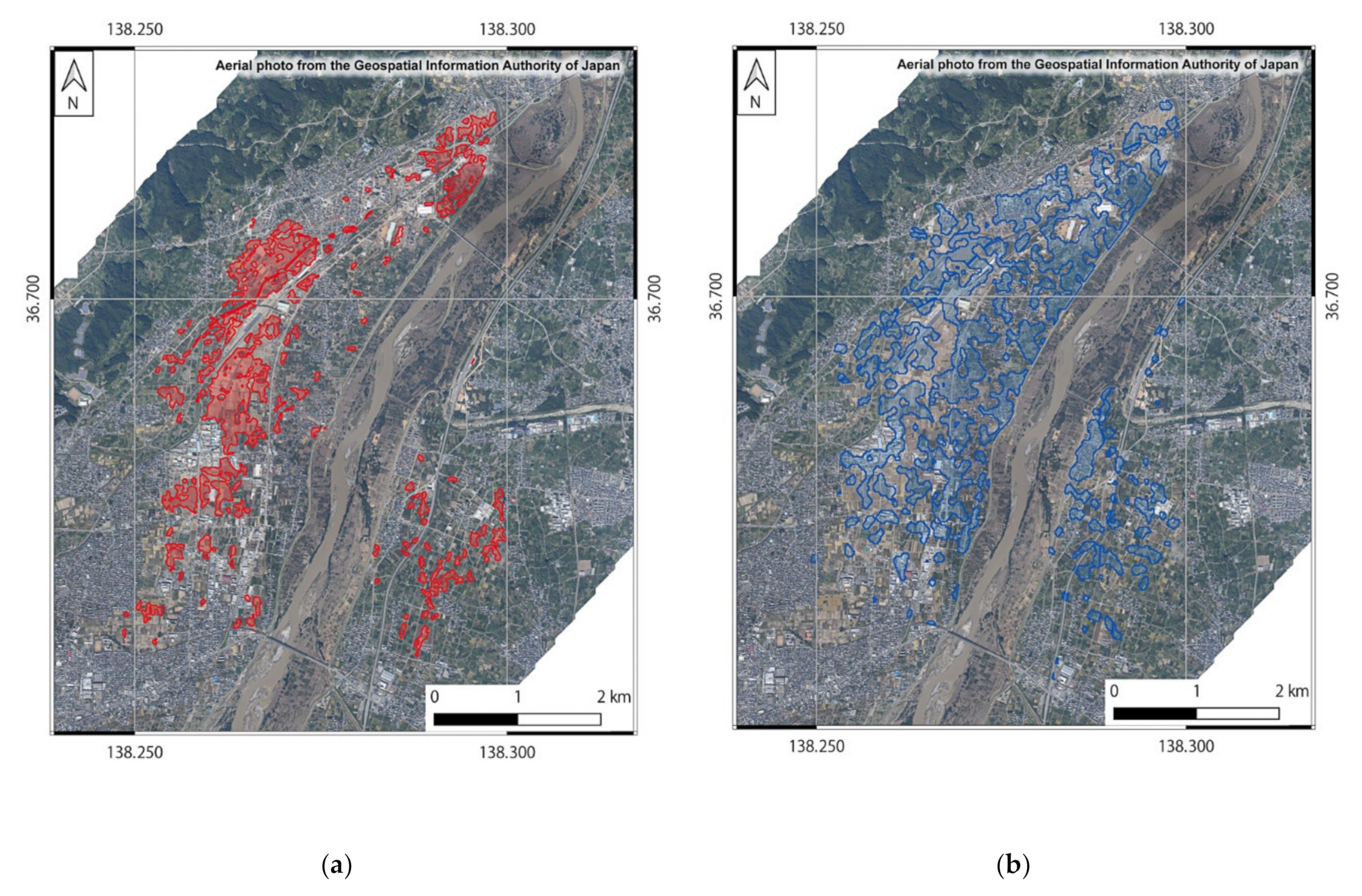
Figure 4a provides the GSI-derived reference inundation domains and
Figure 4b shows an estimated spatial distribution of the water depth provided by GSI.
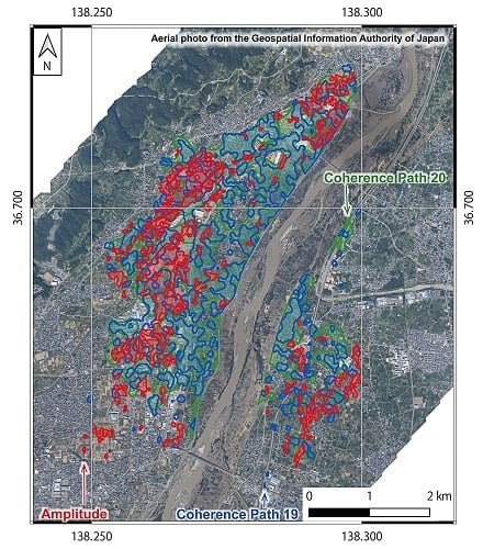
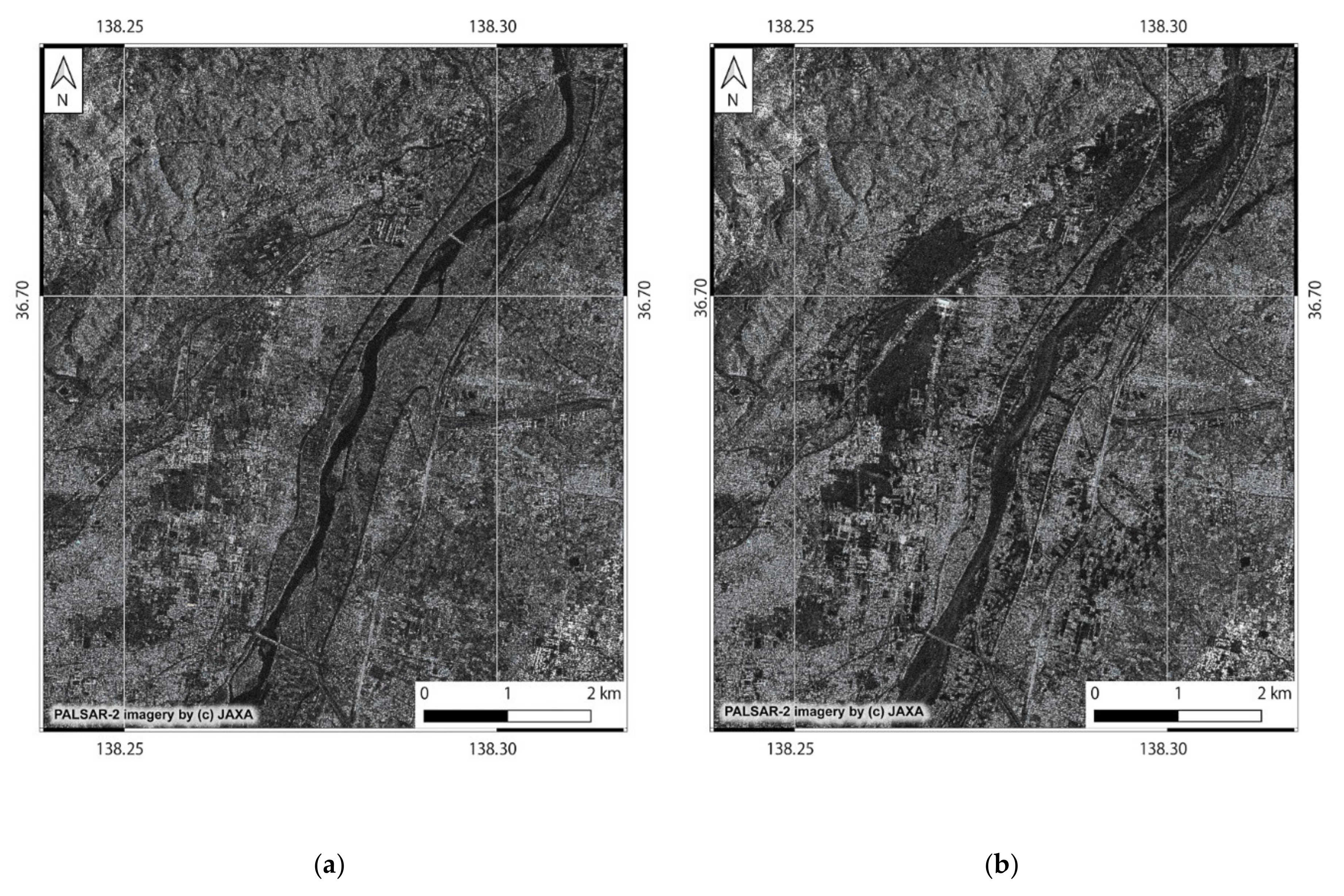
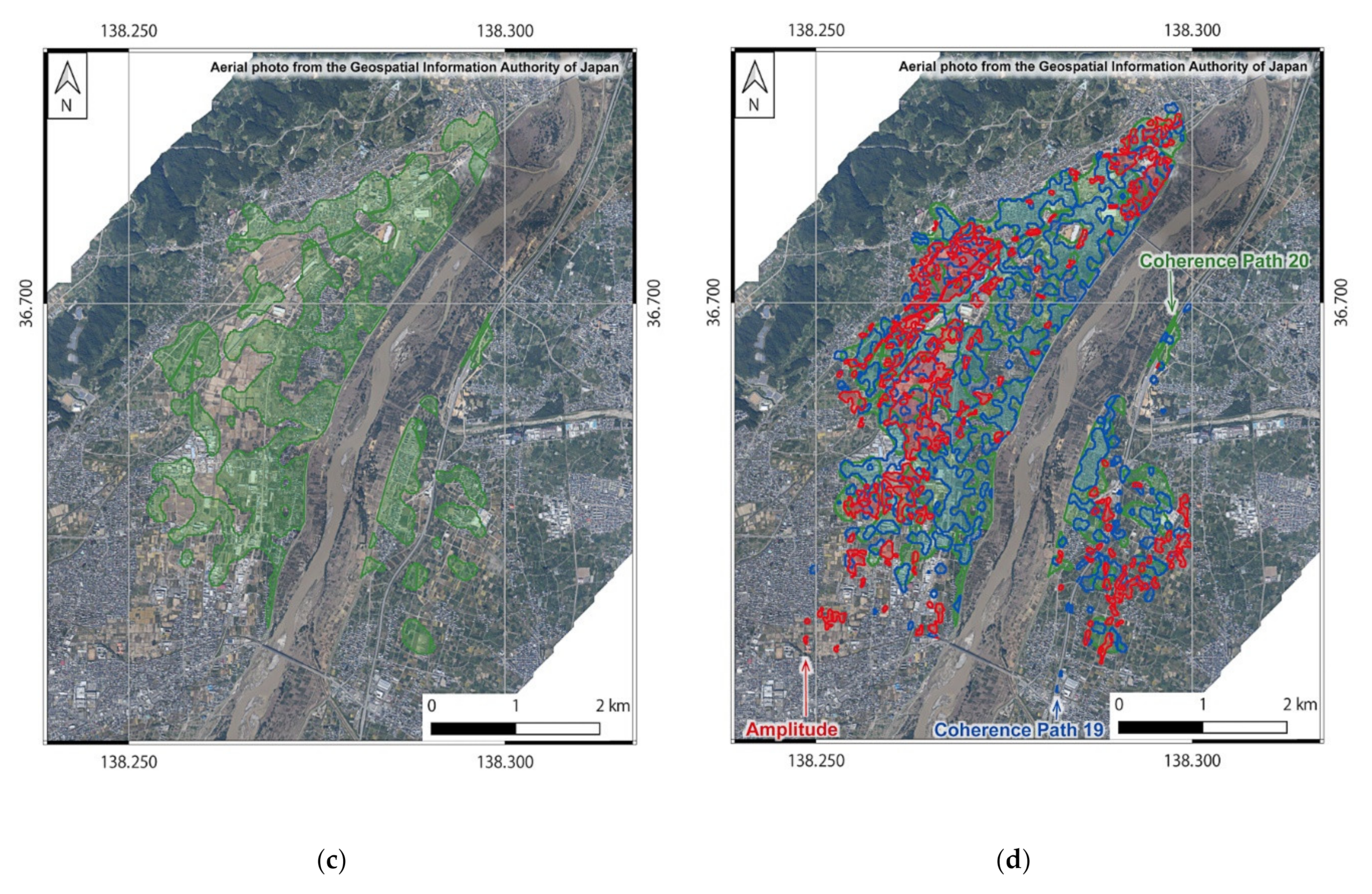
Regarding the land covers and the distribution of flooded areas, we investigated the detection results of the methods used. By comparing the pre-event (
Figure 5a) and post-event (
Figure 5b) intensity images, open water was only detected on the farmland, as shown in
Figure 6a. The train bridge and some buildings increased the intensity, thus prohibiting the detection of the water. This was caused by the double-bounce effect of SAR images, which is typically seen in urban areas [
42,
43]. On the other hand, a current operational digital elevation model (DEM) / digital surface model (DSM), such as SRTM, does not represent the height of the scatterers themselves, thus observing from a different orbit creates a local co-registration error for those scatterers, resulting in a false flood detection alarm. In short, the intensity difference can be caused by an error of the ortho-rectification. Furthermore, in the orchard, sparse trees make it difficult to detect open water. In general, open water decreases the backscattering coefficient, while the trunks and water increase the double bounce occurrence [
15]. In the orchard, open water was hardly visible because of the existing trees, though their density was insufficient for detecting the increase of the intensity.
Interferometric analyses (
Figure 6b,c), on the other hand, could detect the inundation in the orchard. Well-controlled vegetation had a high enough coherence over the seasons, while the rice paddy had a low coherence in the pre-event pair. The observation frequency should be increased to catch the change in the cropland with interferometric methods. In the urban areas, the coherence decrease was successfully detected in both path 19 and path 20 pairs. This was due to the change in the propagation path, and thus, the shallow depth regions were overlooked. The difference in path 19 and path 20 cases could be described in terms of the difference in the orbit and resolution. As the pre-event coherence data from path 19 was made using a traditional Stripmap–Stripmap interferogram, the distribution of the high coherence targets was more localized in the analysis area. Those targets were regarded as flooded by comparing them with the co-event path 20 coherence from the Stripmap–ScanSAR interferogram, while their surrounding low coherence region had a lower coherence decrease, resulting in overlooking the inundation.
Both intensity- and coherence-based analyses were influenced by layover and shadowing, which was emphasized by the difference of the observation paths. The dominant scatterers of the architectures were sometimes on the roof and could not be used to determine whether the area was flooded. Therefore, a more precise analysis and discussion would consider the building heights [
26]. Those reasons that cause the detection ratio to become worse are common with the ideal Stripmap-based analysis. Different observation modes and orbits exaggerate the effect, especially for the producer’s accuracy. In short, what the alternative methods could detect has a high enough accuracy but they may overlook the inundation area. The alternative analyses can become available for analysis under the ideal condition by merging their results.
6. Conclusions
In this paper, we investigated the analysis results of flood detection using space-borne SAR observation in non-ideal conditions. That is, we investigated how the detection accuracy suffered when the pre- and post-event observations were performed with inhomogeneous modes and orbits. In the case of the flood event of the Chikuma River caused by typhoon Hagibis in 2019, the possible dataset contained a pre-event dataset from the neighboring orbit and a different coarser ScanSAR observation mode. The analyses using those alternate datasets suffered by severely overlooking the inundation area. On the other hand, by merging the analytical results using the amplitude and interferometric coherence, the detection accuracy became approximately 80%, which is almost the same rate for, or slightly lower than, the ideal Stripmap-only cases using only a statistical approach.
Author Contributions
R.N. and H.N. jointly designed and performed the experiments; R.N. wrote the draft paper, R.N. and H.N. contributed toward reviewing and editing the paper. All authors have read and agreed to the published version of the manuscript.
Funding
R.N. received a Overseas Research Fellowships grant from the Japan Society for the Promotion of Science (JSPS), no. 201860201.
Acknowledgments
The authors thank the Geospatial Information Authority (GSI) under the Ministry of Land, Infrastructure, Transport and Tourism of Japan for providing the inundation maps and high-resolution aerial imagery. The ALOS-2 original data are copyrighted by the Japan Aerospace Exploration Agency (JAXA) and provided under the JAXA 6th ALOS Research Announcement PI nos. 3044 and 3263. ALOS World 3D is copyrighted by JAXA.
Conflicts of Interest
The authors declare no conflict of interest.
References
- Plank, S. Rapid damage assessment by means of multi-temporal SAR—A comprehensive review and outlook to Sentinel-1. Remote Sens. 2014, 6, 4870. [Google Scholar] [CrossRef] [Green Version]
- Kwak, Y.-J. Nationwide Flood Monitoring for Disaster Risk Reduction Using Multiple Satellite Data. ISPRS Int. J. Geo Inf. 2017, 6, 203. [Google Scholar] [CrossRef]
- Shen, X.; Wang, D.; Mao, K.; Anagnostou, E.; Hong, Y. Inundation Extent Mapping by Synthetic Aperture Radar: A Review. Remote Sens. 2019, 11, 879. [Google Scholar] [CrossRef] [Green Version]
- Cian, F.; Marconcini, M.; Ceccato, P. Normalized Difference Flood Index for rapid flood mapping: Taking advantage of EO big data. Remote Sens. Environ. 2018, 209, 712–730. [Google Scholar] [CrossRef]
- Clement, M.A.; Kilsby, C.G.; Moore, P. Multi-temporal synthetic aperture radar flood mapping using change detection. J. Flood Risk Manag. 2018, 11, 152–168. [Google Scholar] [CrossRef]
- Lin, Y.N.; Yun, S.-H.; Bhardwaj, A.; Hill, E.M. Urban Flood Detection with Sentinel-1 Multi-Temporal Synthetic Aperture Radar (SAR) Observations in a Bayesian Framework: A Case Study for Hurricane Matthew. Remote Sens. 2019, 11, 1778. [Google Scholar] [CrossRef]
- Uddin, K.; Matin, M.A.; Meyer, F.J. Operational Flood Mapping Using Multi-Temporal Sentinel-1 SAR Images: A Case Study from Bangladesh. Remote Sens. 2019, 11, 1581. [Google Scholar] [CrossRef] [Green Version]
- Chini, M.; Pelich, R.; Pulvirenti, L.; Pierdicca, N.; Hostache, R.; Matgen, P. Sentinel-1 InSAR coherence to detect floodwater in urban areas: Houston and Hurricane Harvey as a test case. Remote Sens. 2019, 11, 107. [Google Scholar] [CrossRef] [Green Version]
- Martinis, S.; Kersten, J.; Twele, A. A fully automated TerraSAR-X based flood service. ISPRS J. Photogramm. Remote Sens. 2015, 104, 203–212. [Google Scholar] [CrossRef]
- Giustarini, L.; Hostache, R.; Matgen, P.; Schumann, G.J.P.; Bates, P.D.; Mason, D.C. A change detection approach to flood mapping in urban areas using TerraSAR-X. IEEE Trans. Geosci. Remote Sens. 2013, 51, 2417–2430. [Google Scholar] [CrossRef] [Green Version]
- Chaabani, C.; Chini, M.; Abdelfattah, R.; Hostache, R.; Chokmani, K. Flood mapping in a complex environment using bistatic TanDEM-X/TerraSAR-X InSAR coherence. Remote Sens. 2018, 10, 1873. [Google Scholar] [CrossRef] [Green Version]
- Refice, A.; Capolongo, D.; Pasquariello, G.; D’Addabbo, A.; Bovenga, F.; Raffaele, N.; Lovergine, F.P.; Pietranera, L. SAR and InSAR for flood monitoring: Examples with COSMO-SkyMed data. IEEE J. Sel. Top. Appl. Earth Obs. Remote Sens. 2014, 7, 2711–2722. [Google Scholar] [CrossRef]
- Chini, M.; Pulvirenti, L.; Pierdicca, N. Analysis and interpretation of the COSMO-SkyMed observations of the 2011 Japan tsunami. IEEE Geosci. Remote Sens. Lett. 2012, 9, 467–471. [Google Scholar] [CrossRef]
- Liu, W.; Yamazaki, F. Review article: Detection of inundation areas due to the 2015 Kanto and Tohoku torrential rain in Japan based on multi-temporal ALOS-2 imagery. Nat. Hazards Earth Syst. Sci. 2018, 18, 1905–1918. [Google Scholar] [CrossRef] [Green Version]
- Dabrowska-Zielinska, K.; Budzynska, M.; Tomaszewska, M.; Bartold, M.; Gatkowska, M.; Malek, I.; Turlej, K.; Napiorkowska, M. Monitoring Wetlands Ecosystems Using ALOS PALSAR (L-Band, HV) Supplemented by Optical Data: A Case Study of Biebrza Wetlands in Northeast Poland. Remote Sens. 2014, 6, 1605. [Google Scholar] [CrossRef] [Green Version]
- Manavalan, R. SAR image analysis techniques for flood area mapping - literature survey. Earth Sci. Inform. 2017, 10. [Google Scholar] [CrossRef]
- Pulvirenti, L.; Chini, M.; Pierdicca, N.; Boni, G. Use of SAR data for detecting floodwater in urban and agricultural areas: The role of the interferometric coherence. IEEE Trans. Geosci. Remote Sens. 2015, 54, 1532–1544. [Google Scholar] [CrossRef]
- Rahman, M.S.; Di, L. The state of the art of spaceborne remote sensing in flood management. Nat. Hazards 2017, 85, 1223–1248. [Google Scholar] [CrossRef]
- Tsyganskaya, V.; Martinis, S.; Marzahn, P.; Ludwig, R. SAR-based detection of flooded vegetation–a review of characteristics and approaches. Int. J. Remote Sens. 2018, 39, 2255–2293. [Google Scholar] [CrossRef]
- Yan, K.; Di Baldassarre, G.; Solomatine, D.P.; Schumann, G.J.P. A review of low-cost space-borne data for flood modelling: Topography, flood extent and water level. Hydrol. Process. 2015, 29. [Google Scholar] [CrossRef]
- Schumann, G.J.-P.; Brakenridge, G.R.; Kettner, A.J.; Kashif, R.; Niebuhr, E. Assisting Flood Disaster Response with Earth Observation Data and Products: A Critical Assessment. Remote Sens. 2018, 10, 1230. [Google Scholar] [CrossRef] [Green Version]
- Notti, D.; Giordan, D.; Caló, F.; Pepe, A.; Zucca, F.; Galve, J.P. Potential and limitations of open satellite data for flood mapping. Remote Sens. 2018, 10, 1673. [Google Scholar] [CrossRef] [Green Version]
- Rosser, J.F.; Leibovici, D.G.; Jackson, M.J. Rapid flood inundation mapping using social media, remote sensing and topographic data. Nat. Hazards 2017, 87, 103–120. [Google Scholar] [CrossRef] [Green Version]
- Tanguy, M.; Chokmani, K.; Bernier, M.; Poulin, J.; Raymond, S. River flood mapping in urban areas combining Radarsat-2 data and flood return period data. Remote Sens. Environ. 2017, 198, 442–459. [Google Scholar] [CrossRef] [Green Version]
- Tsyganskaya, V.; Martinis, S.; Marzahn, P.; Ludwig, R. Detection of temporary flooded vegetation using Sentinel-1 time series data. Remote Sens. 2018, 10, 1286. [Google Scholar] [CrossRef] [Green Version]
- Li, Y.; Martinis, S.; Wieland, M.; Schlaffer, S.; Natsuaki, R. Urban Flood Mapping Using SAR Intensity and Interferometric Coherence via Bayesian Network Fusion. Remote Sens. 2019, 11, 2231. [Google Scholar] [CrossRef] [Green Version]
- Bangira, T.; Alfieri, S.M.; Menenti, M.; van Niekerk, A. Comparing Thresholding with Machine Learning Classifiers for Mapping Complex Water. Remote Sens. 2019, 11, 1351. [Google Scholar] [CrossRef] [Green Version]
- Shahabi, H.; Shirzadi, A.; Ghaderi, K.; Omidvar, E.; Al-Ansari, N.; Clague, J.J.; Geertsema, M.; Khosravi, K.; Amini, A.; Bahrami, S.; et al. Flood Detection and Susceptibility Mapping Using Sentinel-1 Remote Sensing Data and a Machine Learning Approach: Hybrid Intelligence of Bagging Ensemble Based on K-Nearest Neighbor Classifier. Remote Sens. 2020, 12, 266. [Google Scholar] [CrossRef] [Green Version]
- Giustarini, L.; Vernieuwe, H.; Verwaeren, J.; Chini, M.; Hostache, R.; Matgen, P.; Verhoest, N.E.C.; de Baets, B. Accounting for image uncertainty in SAR-based flood mapping. Int. J. Appl. Earth Obs. Geoinf. 2015, 34, 70–77. [Google Scholar] [CrossRef]
- Shen, X.; Anagnostou, E.N.; Allen, G.H.; Robert Brakenridge, G.; Kettner, A.J. Near-real-time non-obstructed flood inundation mapping using synthetic aperture radar. Remote Sens. Environ. 2019, 221, 302–315. [Google Scholar] [CrossRef]
- Plank, S.; Jüssi, M.; Martinis, S.; Twele, A. Mapping of flooded vegetation by means of polarimetric sentinel-1 and ALOS-2/PALSAR-2 imagery. Int. J. Remote Sens. 2017, 38, 3831–3850. [Google Scholar] [CrossRef]
- Martinis, S.; Rieke, C. Backscatter Analysis Using Multi-Temporal and Multi-Frequency SAR Data in the Context of Flood Mapping at River Saale, Germany. Remote Sens. 2015, 7, 7732. [Google Scholar] [CrossRef] [Green Version]
- Martinis, S.; Kuenzer, C.; Wendleder, A.; Huth, J.; Twele, A.; Roth, A.; Dech, S. Comparing four operational SAR-based water and flood detection approaches. Int. J. Remote Sens. 2015, 36, 3519–3543. [Google Scholar] [CrossRef]
- Landuyt, L.; Van Wesemael, A.; Schumann, G.J.P.; Hostache, R.; Verhoest, N.E.C.; Van Coillie, F.M.B. Flood Mapping Based on Synthetic Aperture Radar: An Assessment of Established Approaches. IEEE Trans. Geosci. Remote Sens. 2019, 57, 722–739. [Google Scholar] [CrossRef]
- Li, Y.; Martinis, S.; Plank, S.; Ludwig, R. An automatic change detection approach for rapid flood mapping in Sentinel-1 SAR data. Int. J. Appl. Earth Obs. Geoinf. 2018, 73, 123–135. [Google Scholar] [CrossRef]
- Benoudjit, A.; Guida, R. A novel fully automated mapping of the flood extent on sar images using a supervised classifier. Remote Sens. 2019, 11, 779. [Google Scholar] [CrossRef] [Green Version]
- Japan Meteorological Agency, Typhoon Hagibis Response Site (In Japanese). Available online: http://www.jma.go.jp/jma/en/201910_Heavyrain/2019_Heavyrain.html (accessed on 21 December 2019).
- Geospatial Information Authority of Japan, Typhoon Hagibis Response Site (In Japanese). Available online: https://www.gsi.go.jp/BOUSAI/R1.taihuu19gou.html (accessed on 21 December 2019).
- Japan Aerospace Exploration Agency (JAXA), ALOS-2 CEOS-SAR Product Format. Available online: https://www.eorc.jaxa.jp/ALOS-2/en/doc/format.htm (accessed on 10. March 2019).
- Ohki, M.; Tadono, T.; Itoh, T.; Ishii, K.; Yamanokuchi, T.; Watanabe, M.; Shimada, M. Flood Area Detection Using PALSAR-2 Amplitude and Coherence Data: The Case of the 2015 Heavy Rainfall in Japan. IEEE J. Sel. Top. Appl. Earth Obs. Remote Sens. 2019, 12, 2288–2298. [Google Scholar] [CrossRef]
- Natsuaki, R.; Motohka, T.; Watanabe, M.; Ohki, M.; Thapa, R.B.; Nagai, H.; Tadono, T.; Shimada, M.; Suzuki, S. Emergency Observation and Disaster Monitoring Performed by ALOS-2 PALSAR-2. In Proceedings of the IEEE International Geoscience and Remote Sensing Symposium, Beijing, China, 10–15 July 2016. [Google Scholar]
- Arii, M.; Yamada, H.; Kojima, S.; Ohki, M. Review of the Comprehensive SAR Approach to Identify Scattering Mechanisms of Radar Backscatter from Vegetated Terrain. Electronics 2019, 8, 1098. [Google Scholar] [CrossRef] [Green Version]
- Moya, L.; Endo, Y.; Okada, G.; Koshimura, S.; Mas, E. Drawback in the Change Detection Approach: False Detection during the 2018 Western Japan Floods. Remote Sens. 2019, 11, 2320. [Google Scholar] [CrossRef] [Green Version]
© 2020 by the authors. Licensee MDPI, Basel, Switzerland. This article is an open access article distributed under the terms and conditions of the Creative Commons Attribution (CC BY) license (http://creativecommons.org/licenses/by/4.0/).


