Estimating Meltwater Drainage Onset Timing and Duration of Landfast Ice in the Canadian Arctic Archipelago Using AMSR-E Passive Microwave Data

Abstract

Meltwater drainage onset (DO) timing and drainage duration (DD) related to snowmelt-water redistribution are both important for understanding not only the Arctic energy and heat budgets but also the salt/heat balance of the mixed layer in the ocean and sea-ice ecosystem. We present DO and DD as determined from the time series of Advanced Microwave Scanning Radiometer-Earth observing system (AMSR-E) melt pond fraction (MPF) estimates in an area with Canadian landfast ice. To address the lack of evaluation on a day-by-day basis for the AMSR-E MPF estimate, we first compared AMSR-E MPF with the daily Medium Resolution Imaging Spectrometer (MERIS) MPF. The AMSR-E MPF estimate correlates significantly with the MERIS MPF (r = 0.73–0.83). The estimate has a product quality similar to the MERIS MPF only when the albedo is around 0.5–0.7 and a positive bias of up to 10% in areas with an albedo of 0.7–0.9, including melting snow. The DO/DD estimates are determined by using a polynomial regression curve fitted on the time series of the AMSR-E MPF. The DOs/DDs from time series of the AMSR-E and MERIS MPFs are compared, revealing consistency in both DD and DO. The DO timing from 2006 to 2011 is correlated with melt onset timing. To the best of our knowledge, our study provides the first large-scale information on both DO timing and DD.

1. Introduction

The surface melt of Arctic sea ice begins in early summer, with liquid water pools (called melt ponds) forming on the ice. These melt ponds reduce the regional albedo, enhance heat uptake on the sea ice [1], and have an impact on simulations of an accelerating under-ice melt [2,3]. Schröder et al. [4] found that an accurate accounting of melt ponds during the melt season leads to better predictions of sea ice extent in the fall. Thus, a better understanding of the temporal and spatial variability in melt pond fraction (MPF) facilitates an investigation of the function of melt ponds in the Arctic and in the earth’s climate system [5,6,7].

A critical component of the time series of the MPF is the existence of pathways for meltwater drainage to sea level through the sea ice. The MPF is largely controlled by a hydraulic balance of meltwater inflows and outflows [8,9] (Figure 1). The first part of the melt season is characterized by a dominant lateral meltwater flow, widespread pond coverage, and a rapid increase in MPF [8]. Later, in the second part of the melt season, meltwater drainage occurs mainly by the lateral flow of meltwater across the ice surface, toward macroscopic flaws such as brine drainage channels, ice floe edges, and cracks. Then the snow cover melts completely, concurrent with a reduction in MPF and enhancement of albedo [8,9]. In the third part of the melt season, sea ice has high permeability and open macroscopic flaws, which accelerate ice floe breakup and disintegration [8]. The permeability of multiyear ice (MYI) is lower than that of first-year ice (FYI), and the low permeability of MYI helps to retain meltwater on the sea ice’s surface [10,11]. In the last part of the melt season, the surface of the melt pond freezes in cases where sea ice remains throughout the melt season [8]. Meltwater drainage (particularly on MYI) does not always occur or slowly occurs, meaning that meltwater remains on the surface throughout the melt season, that there may be no sharp boundary for onset and offset, and that the meltwater surface eventually freezes in the fall freeze-up period (Figure 1b).

The first and second parts of the melt season, characterized as having a very low albedo and a near peak of annual insolation, have a particularly large impact on the surface energy balance [9]. Then, sea ice melting is promoted by a positive permeability/heat-flux feedback, resulting in abundant meltwater drainage into highly permeable ice, particularly FYI [8,9]. Meltwater of low salinity and low nutrient concentrations is also retained under ice or in bottom depressions, forming under-ice freshwater lenses (i.e., under-ice melt ponds). The redistribution of meltwater affects the salt and heat balance at the layer where fresh meltwater and saline water mix [12], and the supply of atmospheric pollutants into the ocean and the sea-ice ecosystem [13]. Understanding the drainage onset (DO) timing and drainage duration (DD) related to meltwater redistribution in the early melt season will help to model changes in physical and biological coupling within the Arctic sea ice ecosystem.

An understanding of DO and DD is often achieved through both airborne and in situ measurements [8,9,10,11,14], although this is difficult at larger scales for temporal and spatial limitations. Satellite passive microwave and optical remote sensing is useful for monitoring the entire polar regions daily [15,16], although optical remote sensing is limited by cloud cover when observing sea ice conditions. Although the timing of melt onset (MO) has been derived using passive microwave remote sensing [17,18,19,20], little is known about large-scale DO timing and DD in the melt season.

This study aims to derive this DO and DD using the time series of MPF retrieved data from the Advanced Microwave Scanning Radiometer-Earth observing system (AMSR-E MPF), an estimate proposed by Tanaka et al. [21] (see Supplementary Text S1). The AMSR-E MPF estimate is valid in the Beaufort Sea with pack ice and Canadian Arctic Archipelago (CAA) areas with landfast ice. To determine the DO and DD, only the CAA region with landfast ice was chosen for this study since the same sea ice needs to be observed during the melt season. To avoid the contamination of open water in the AMSR-E MPF estimate, we used a totally ice-covered area (10/10 ice concentration), without open water contamination in the AMSR-E MPF estimate until the breakup of landfast ice using ice charts, available from 2006 to present (Section 2.1). To address the lack of evaluation on a day-by-day basis for the AMSR-E MPF estimate (see Supplementary Text S2), we first compare the AMSR-E MPF to the daily MPF product from the Medium Resolution Imaging Spectrometer (MERIS MPF) and then discuss the biases related to melting snow in the early melt season. Results from the six-year period of 2006–2011 are used for both evaluation and examination. Data from the AMSR2 sensor, which superseded the AMSR-E sensor, on the Global Change Observation Mission 1st-Water (GCOM-W1) satellite will extend the continuous record of the MPF, DO, and DD from 2012 to present, when the MPF retrieved from AMSR2 data is evaluated in a future paper.

2. Data and Methods

2.1. Canadian Ice Service Regional Ice Charts

Figure 2 is a map of our study area, including the CAA and its subregions. This also shows the extent of AMSR-E data and the products of MPF and spectral sea ice albedo from MERIS data, as discussed in the next subsection. To obtain total ice concentration data in the CAA, we used the Canada Ice Service (CIS) weekly ice charts in Sea Ice Geo Referenced Information and Data (SIGRID)-3 format [22], including total sea ice concentration from 2006 to 2011 [23]. The ice charts were created based on the Manual of Standard Procedures for Observing and Reporting Ice Conditions (MANICE) [24] and were prepared by following internationally recommended terminology and symbology established by the World Meteorological Organization (WMO). The ice charts from 2006 to the present were created manually by the CIS based on various satellite data, aerial reconnaissance, ship reports, and operational model results and then made available through the National Snow and Ice Data Center (NSIDC). These data are provided in six different regions, but this study used only charts from the Western and Eastern Arctic regions, as shown in Figure 2. SIGRID-3 data are in ESRI shapefile format, following the JCOMM convention [22]. Supplementary Text S3 summarizes the main sources of error in the ice charts described by Tivy et al. [25].

The ice charts used by Tanaka et al. [21] were paper maps, using areas with “9+/10” and “10/10”. Each area is defined as having a sea ice concentration exceeding 95%, which was manually extracted. The ice charts in this study provide three sea ice concentration ranges of “9–10/10”, “9+/10”, and “10/10” as one code. To avoid the contamination of open water in the AMSR-E MPF estimate, we used only the totally ice-covered areas with landfast ice (10/10 sea ice concentration). The ice charts were resampled into 25 km × 25 km NSIDC stereographic projection grids (NSIDC grids).

2.2. Satellite Data Product

We used the daily brightness temperature (T_B) in the AMSR-E/Aqua Daily L3 25 km polar stereographic product provided by the NSIDC for the AMSR-E MPF estimate. The AMSR-E operated from 2002 to 2011 and was a passive microwave radiometer on NASA’s Aqua satellite, equipped with 12 channels at 6.9, 10.7, 18.7, 23.8, 36.5, and 89.0 GHz, including both vertical (V) and horizontal (H) polarizations. It provided data in both ascending and descending (morning and evening) orbits. The spatial resolutions of individual frequencies ranged from 4 km × 6 km at 89.0 GHz to 43 km × 75 km at 6.9 GHz. In the product, the resampling interval is 25 km × 25 km at all frequencies. We used the daily average, T_B, and only the H polarization channel at 6.9 GHz and the V polarization channel at 89 GHz. The input data for the latest version 3 T_B product are the AMSR-E L2A Global Swath Spatially Resampled Brightness Temperatures product, including land contamination. The contamination impact on T_B (particularly at 6.9 GHz) near shore results from the fact that T_B is higher over land than sea. Tanaka et al. [21] found that an increase in the T_B at 6.9 GHz means a decrease in the MPF. Therefore, land contamination may lead to a lower MPF near the shore. We used the DMSP SSM/I-SSMIS Daily Polar Gridded Brightness Temperatures Version 5 product provided by the NSIDC, to determine the freeze onset (FO) date. We used only the T_Bs from 2006 to 2011, with V polarization at 19 and 37 GHz.

For evaluating the AMSR-E MPF from 2006 to 2011, we used the evaluation product, which consists of daily averaged MPFs, and broadband albedo, using the 12.5 km NSIDC grid with the criterion of more than 50% valid pixels (both spatially and temporally). This period corresponds to the availability period of the ice chart data (Section 2.1). The product was made based on the swath MERIS Level 1b data with 1 km × 1 km spatial resolution over the Arctic summers from 2002 to 2011. The MPF data were obtained by the melt pond detector (MPD) algorithm [16]. The 12.5 km NSIDC grid is projected onto the 25 km NSIDC grid, which averages by using four of the 12.5 km NSIDC grid cells. All comparisons were made using the 25 km NSIDC grid. Supplementary Text S4 summarizes the characteristics of the products of MPF and spectral sea ice albedo from MERIS data [26,27].

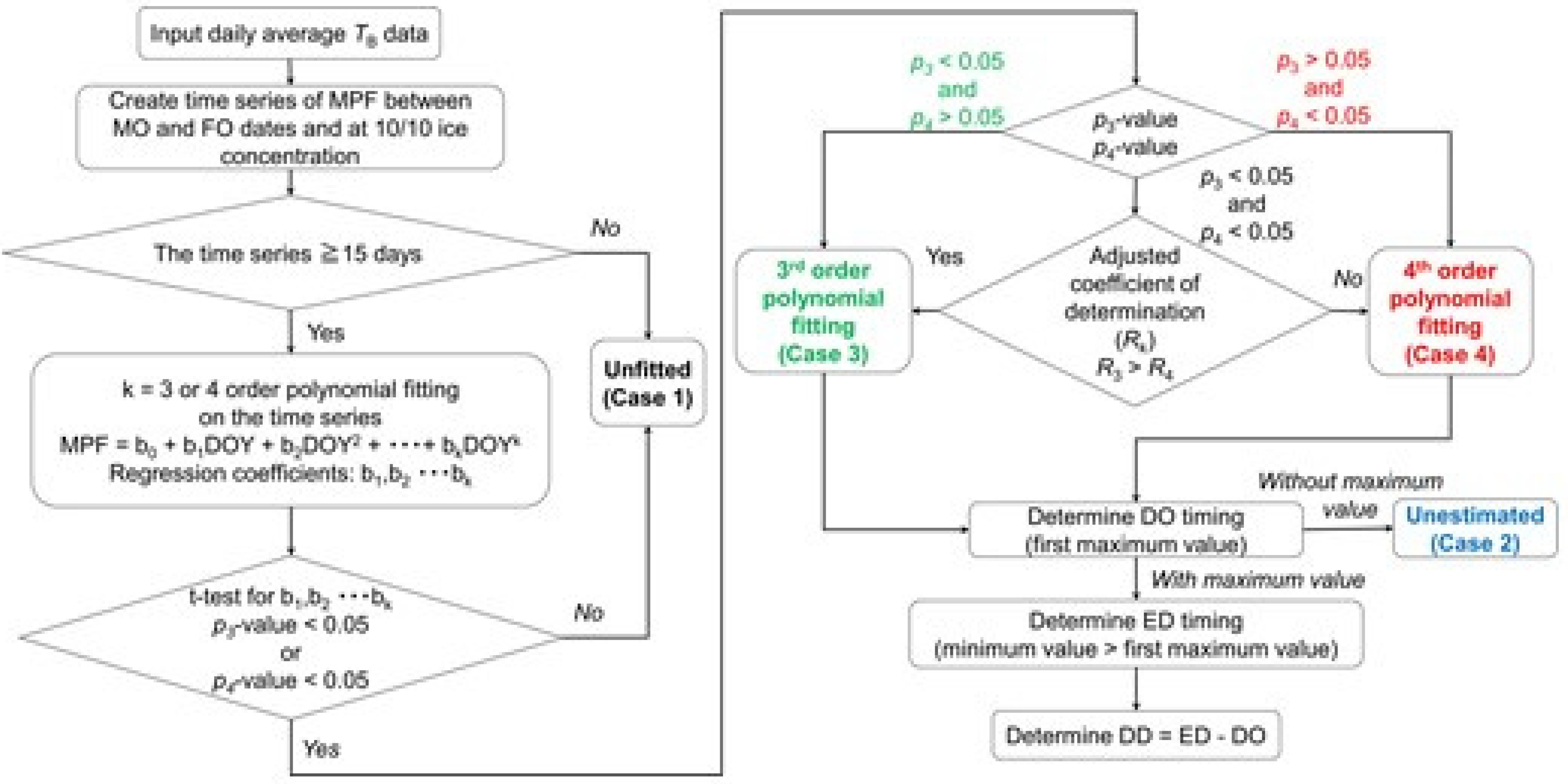
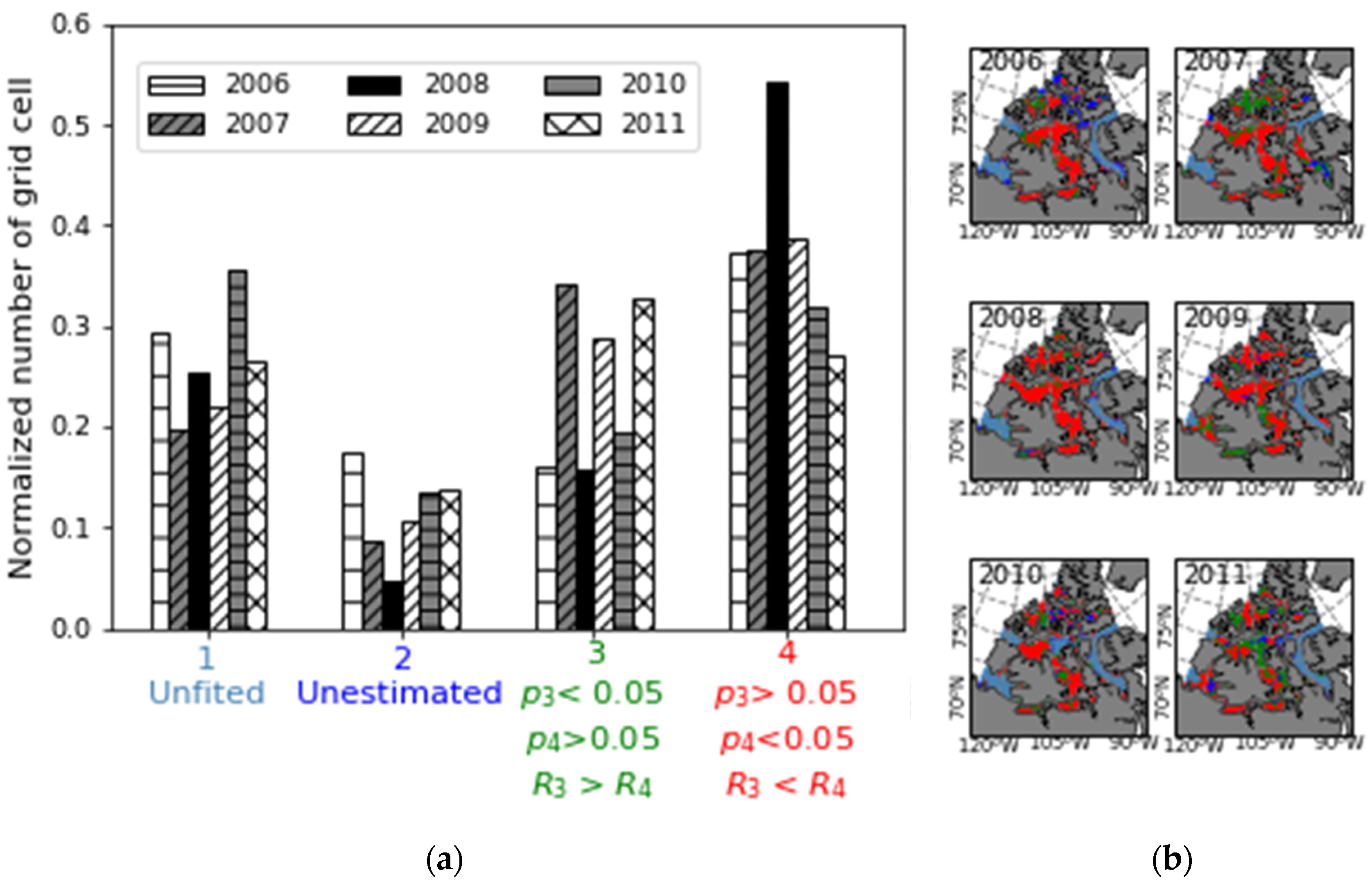
2.3. Estimating Meltwater Drainage Onset Timing and Duration

As an example, we show how to determine the DO timing and DD by using the six points plotted in Figure 2. Figure 3 shows the time series of the AMSR-E MPF and daily average 2 m air temperature in the ERA5 dataset provided by the European Centre for Medium-Range Weather Forecasts (ECMWF, https://www.ecmwf.int/). The MO date is obtained by using the dynamic threshold variability method based on 36.5 GHz vertically polarized T_B data [20]. The FO date is retrieved from the melt/freeze-up algorithm, using 19 and 37 GHz vertically polarized T_B data [18]. As previously stated, the MPF after MO rapidly increases, and later, when the MPF decreases temporally, is when an increase in ice permeability or meltwater drainage occurs (Figure 1). This feature was also found in the time series of the AMSR-E MPF (black circles in Figure 3d–f) and then used to estimate the most likely DO timing and DD. Figure 4 is a flowchart of the method for estimating DO timing and DD, relative to the following five steps:

(1) The time series of the MPF is created from the AMSR-E MPF estimation method. The time series in Figure 3 includes MPF estimates outside the conditions when melt ponds are expected to occur, i.e., prior to MO: the gray circles in Figure 3 after the FYI completely melts or breaks up and there is open water (gray x’s in Figure 3), and after the FO. These data points outside the possible melt season are problematic and are not to be included; we only used the realistic time series over 10/10 ice concentration and between the MO and FO dates, as the black circles in Figure 3 show. If the threshold of the MO is not determined due to the high inter-quartile range in the histogram of the potential MO [20], a data point of more than 0 °C air temperature is used for determining a realistic time series.

(2) The time series can be expressed accurately as a third or fourth order function, as shown in Figure 1. We assume a third or fourth (k = 3 or 4) order polynomial regression in one variable, y = b₀ + b₁x + b₂x²…+ b_kx ^k, where y (MPF) is the predicted outcome of the polynomial regression. The regression coefficients are b₁ to b_k for each order, where b₀ is the y-intercept, and x (day of year, DOY) is an explanatory variable. To examine the significance of b₁ to b_k, we determine p_k-values for all coefficients of the k = 3 or 4 (p₃ and p₄, respectively). If p₃ > 0.05 and p₄ > 0.05, the grid cell is defined as an unfitted case (Case 1).

(3) The time series is fitted with k = 3 if p₃ < 0.05 and p₄ > 0.05, and with k = 4 if p₃ > 0.05 and p₄ < 0.05. If both p₃ and p₄ are less than 0.05, k is determined by using the degree of freedom adjusted coefficient of determination (R_k).

(4) The maximum and minimum values are detected on the k = 3 or 4 order regression curves. In [8,9], the first maximum was taken as the DO date, and the first minimum was taken as the end-of-drainage (ED) date (i.e., the onset of melt pond evolution). Following these, we defined the first maximum as the DO and the first minimum as the ED posterior to the maximum, on the curves. If there are no maximum values, the dates are not estimated for that cell (Case 2).

(5) Finally, DD is calculated from the difference between ED and DO.

Figure 5 shows a histogram and the spatial distributions for each case. Case 1 is 20%–35% of all grid cells and is distributed in the West Arctic Waterway, Baffin Inlet, and East Parry Channel. This is because a passive microwave signal has difficulty distinguishing between saline seawater and freshwater in ponds in cold-water regions when the first-year ice is completely melting or breaking up (Figure 3a) and low significance of the k associated with high variability of the time series (Figure 3b). Case 2 is around 10%. Case 3 (k = 3 regression) is 20%–40%, and the realistic time series is broken by contamination of open water after the ED timing. Case 4 (k = 4 regression) is 30%–55%. The time series in Figure 3e (similar to that in Figure 3d) incorporates k = 4 regression. This case needs a higher k because the variability of the time series is higher for Figure 3e than Figure 3d. The difference in variability between Case 3 and Case 4 areas may be due to melting snow coverage or land contamination on the T_B (particularly for the coarse spatial resolution at 6.9 GHz).

3. Results and Discussion

Figure 6a–f shows the relationship between the MERIS and AMSR-E MPFs from 2006 to 2011. We show only the relationship over 10/10 ice concentration and from the MO date to the FO date. The data of AMSR-E MPFs strongly correlated with those of MERIS MPFs with r = 0.73−0.83 and a root mean square error (RMSE) of 8–9%. The AMSR-E MPF estimates in areas less than 10%–20% and ranging from 20% to 50% overestimate and underestimate the MERIS MPF estimates, respectively. The lower MPFs were biased toward the positive, and the higher MPFs were biased toward the negative, meaning that the negative and positive biases largely cancel each other out. This leads to the low bias of ±2% from 2006 to 2011. The biases strongly correlated with an average albedo with r = 0.68−0.96 at the 99% confidence level (Figure 6g).

Microwave radiometric properties are influenced by sea ice condition between the melt ponds and by melting snow outside melt ponds (e.g., prior to). We now discuss this effect on the AMSR-E MPF estimate. Different ice conditions during the melt season are often summarized as broadband albedos [28,29,30], so we determined three categories according to the broadband albedo obtained from the products of MPF and spectral sea ice albedo from MERIS data, as follows: melting snow between the ponds or melting snow outside ponds for an albedo > 0.7; bare ice including light ponds for an albedo of 0.6–0.7; and ponded ice for an albedo of 0.3–0.6. Figure 6g shows the bias at each albedo with 0.02 bin size from 2006 to 2011. The areas over 10/10 ice concentration and from the MO to FO dates are used to obtain the average bias at each albedo. The biases for an albedo between 0.4 and 0.5 were negative and close to zero around albedo of 0.5. At an albedo between 0.5 and 0.7, the biases were around zero and constant, and they shifted from negative to positive at an albedo over 0.7. The largest positive/negative biases were at an albedo of 0.7–0.9/around 0.4. We found that the AMSR-E MPFs in areas with an albedo of 0.7–0.9 (including melting snow) are 10% larger than the MERIS MPFs, and that bare ice shows little bias compared to the MERIS MPF. T_B decreases at 6.9 GHz and increases at 89.0 GHz, with an increase in the MPF, meaning that the gradient ratio GR_06H–89V decreases with an increase in the MPF [21]. When dry snow starts to melt, the T_B also decreases around 6 GHz and increases around 89 GHz. Therefore, we consider that an increase of snow wetness on sea ice probably led to a positive bias (an increase of pseudo-AMSR-E MPF). After all the snow was gone, there were few biases in the area with an albedo of 0.5–0.7. This suggests that the AMSR-E MPF product provides a quality product, similar to the MERIS MPF, only when the albedo is around 0.5–0.7. The negative biases to 20% were apparent around an albedo of 0.4–0.5. The AMSR-E MPF estimate is mostly useful after snow cover has melted completely. In contrast, the reflectance of wet ice is very close to that of a melt pond [16], so this too may lead to an increase of pseudo-MERIS MPF. We can conclude that an increase in wet ice leads to negative biases.

The DOs/DDs from the time series of the AMSR-E and MERIS MPFs are compared. Here we used 1954 datapoints on a number of AMSR-E and co-located MERIS grid cells. Figure 7 shows the differences between DOs/DDs from the time series of the AMSR-E and MERIS MPFs. These differences show a normal distribution. The mode and average of the DO/DD differences were 2.0/–2.0 days and 2.1/–3.4 days, respectively, with a standard deviation of 6.6/6.0 days, indicating that DO and DD are consistent.

We show maps of the MO timing (Supplementary Figure S1), DO timing (Figure 8), and DD (Figure 9), from 2006 to 2011. Results from the CAA and seven subregions are summarized by averaging the 2006–2011 data (Supplementary Table S1). The average date of DO in the CAA was 177 DOY, with a standard deviation of 9 days. On average from 2006 to 2011, the earliest and the latest DO dates were 171 DOY in the West Arctic Waterway and 182 DOY in the QEI, respectively (Figure 8a). The standard deviations of DO timing were higher in the QEI and West Parry Channel, and lower in other subregions (Figure 8b). The determinations of DO timing and DD in the East Parry Channel were limited by the contamination of open water in the AMSR-E MPF estimate from earlier melt seasons. In each year, contrasts in the DO timing between the QEI and the other six regions in 2006, 2009, and 2010 (Figure 8c,f,g) were higher than those in 2007, 2008, and 2011 (Figure 8d,e,h). The characteristics of both high and low contrasts were found in the map of MO timing (Supplementary Figure S1). We compared the averaged MO timings to the averaged DO timings. The value of r for MO and DO indicated a strong relationship (r = 0.77, p-value < 0.001). The scatterplot for the East Parry Channel in the relationship between the averaged MO timing and the averaged DO timing was far from the linear regression line (not shown). This may limit determining the DO timing. The correlation increases to r = 0.91 (p-value < 0.001) without any points in the East Parry Channel, so that the average DO timing follows the average MO timing in the subregions. The determination of DDs in the East Parry Channel and Baffin Inlet was also limited by the contamination of open water. We exclude data from the East Parry Channel and Baffin Inlet. The average DD in the CAA was 13 days with a standard deviation of nine days (Figure 9a,b). The shortest and longest DDs were 11 days in the West Parry Channel and 17 days in the QEI, respectively.

According to [8,9,10,11], FYI and MYI have higher and lower permeabilities, respectively, and active horizontal flow, particularly in level ice, during low ice permeability, leads to meltwater into macroscopic pathways, such as seal breathing holes and cracks. Therefore, the variability of DO timing and DD in each year may be associated with sea ice type and roughness. To explain the relationship between the variability and sea ice type or roughness, time series of AMSR2 MPF from 2012 to present is required for long-term records of the MPF, DO timing, and DD.

4. Conclusions

This study leads to following results:

(1)

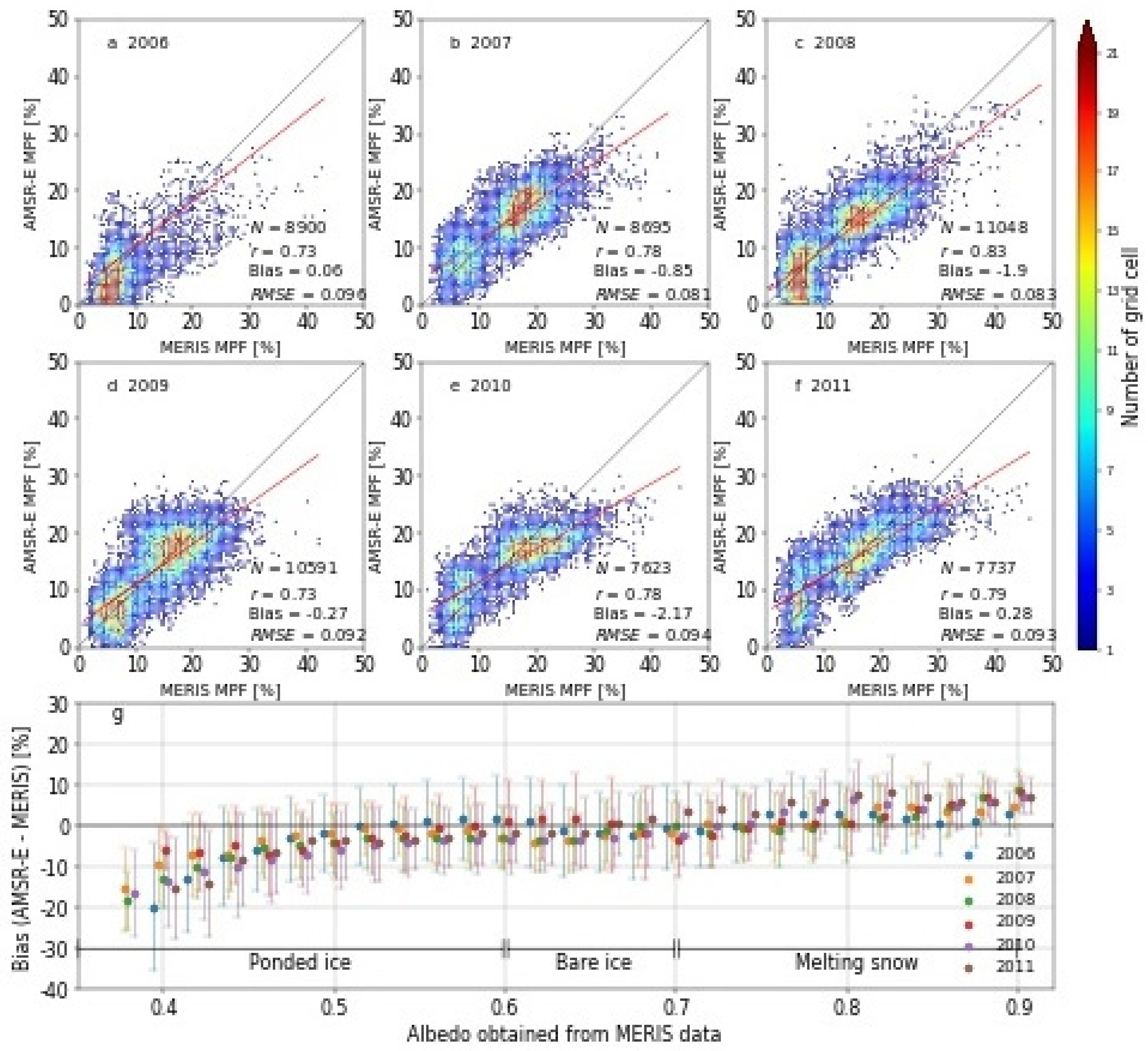
We evaluated the AMSR-E MPF estimate [21] by using daily average T_B for the AMSR-E L3 25 km NSIDC grid data in the CAA, compared it to the daily MERIS MPF in the CAA, and found that the relationship between AMSR-E and MERIS MPFs showed a strong correlation of 0.73–0.83, with a low bias of ±2% and RMSE of 8–9%, from 2006 to 2011. Moreover, the AMSR-E MPFs are 10% larger than the MERIS MPFs due to areas with albedos of 0.7–0.9, including melting snow until the snow cover melted away. Our evaluation demonstrated that the AMSR-E MPF product provides a quality product, similar to the MERIS MPF, only when the albedo is around 0.5–0.7.

(2)

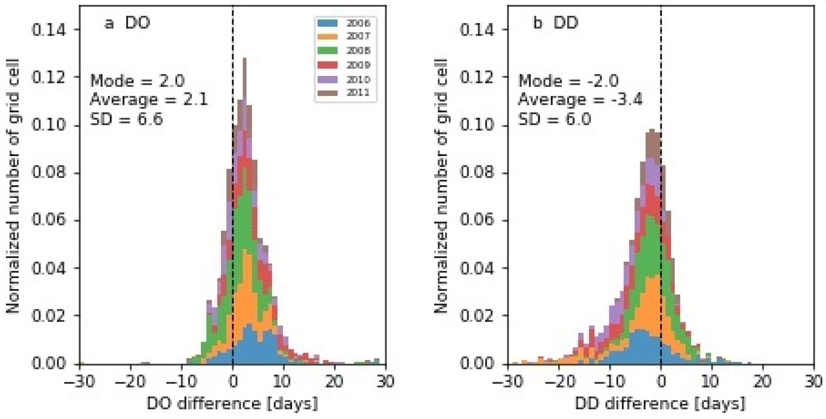
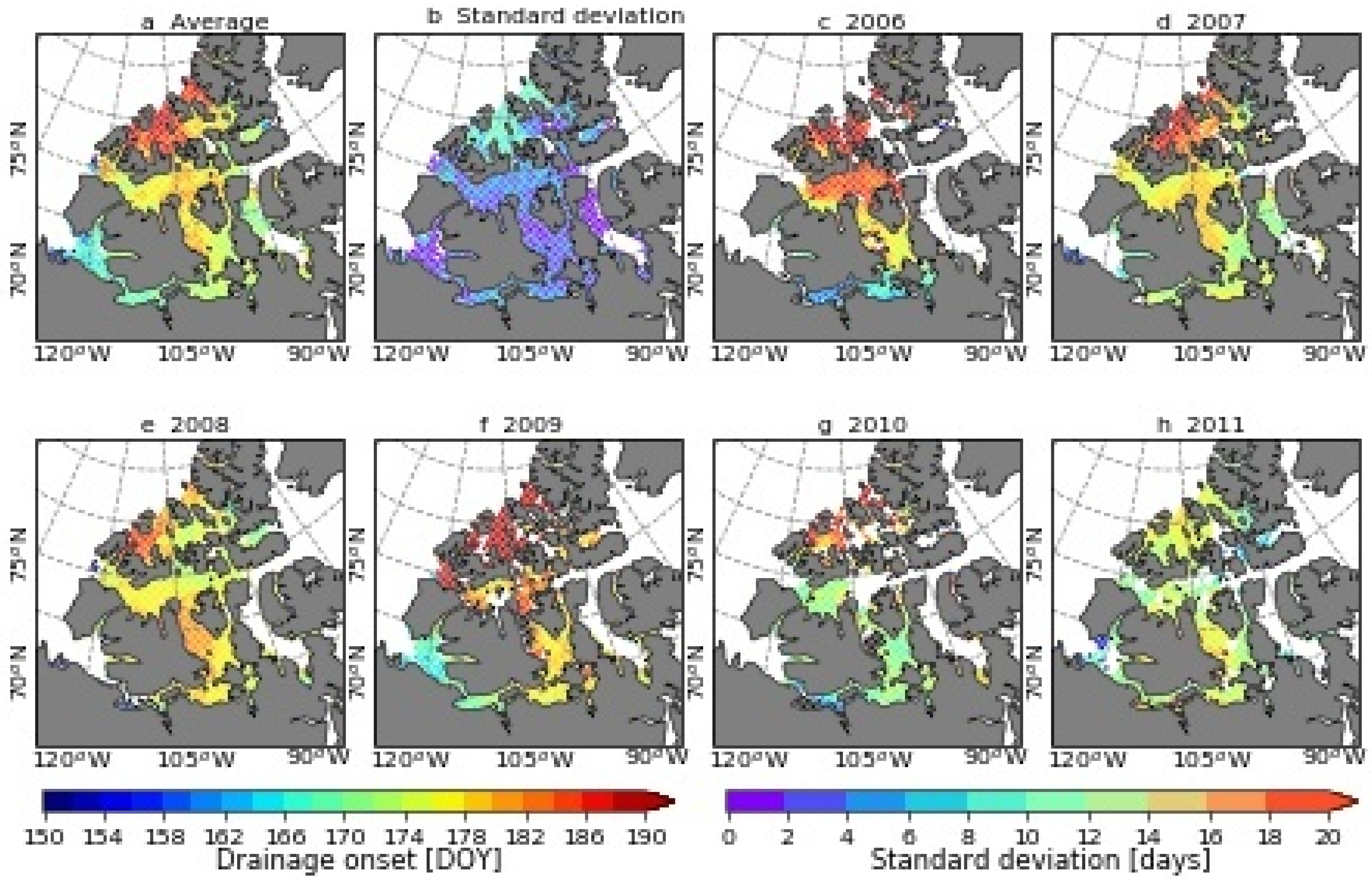
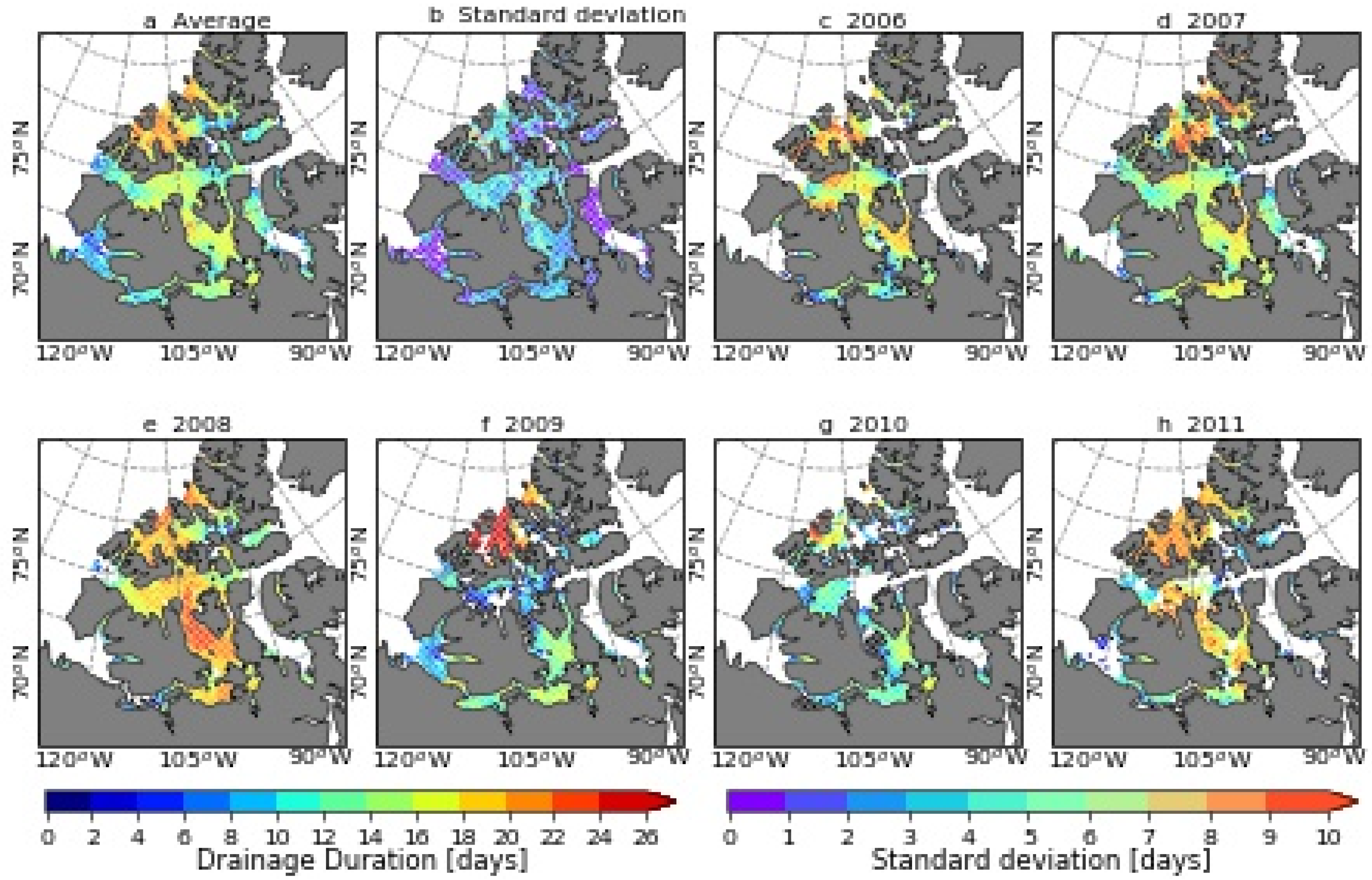
We determined the DO/DD by using polynomial regression curves fitted on a time series of the AMSR-E MPF. The DOs/DDs from the time series of the AMSR-E and MERIS MPFs were compared, resulting in the finding that both DD and DO were consistent. Upon examining the average DO/DD in the subregions from 2006 to 2011, we found that the DO timing averaged in each subregion may correlate with the average MO timing.

To the best of our knowledge, our study provides the first large-scale collection of information of both DO timing and DD. Our attempts were limited by the AMSR-E MPF estimate, which is based on the empirical linear equation, using the AMSR-E T_B data. For example, it is difficult to find trends in DO timing and DD since the time series of AMSR-E MPF is short. Further evaluation of the AMSR2 MPF estimate is required for time series of MPF from 2012 to the present.

References

1. Fetterer, F.; Untersteiner, N. Observations of melt ponds on Arctic sea ice. J. Geophys. Res. 1998, 103, 24821–24835. [Google Scholar] [CrossRef]
2. Perovich, D.K.; Light, B.; Eicken, H.; Jones, K.F.; Runciman, K.; Nghiem, S.V. Increasing solar heating of the Arctic ocean and adjacent seas, 1979–2005, Attribution and role in the ice-albedo feedback. Geophys. Res. Lett. 2007, 34, L19505. [Google Scholar] [CrossRef] [Green Version]
3. Inoue, J.; Curry, J.A.; Maslanik, J.A. Application of aerosondes to melt-pond observations over Arctic sea ice. J. Atmos. Oceanic Technol. 2008, 25, 272334. [Google Scholar] [CrossRef]
4. Schröder, D.; Feltham, D.L.; Flocco, D.; Tsamados, M. September Arctic sea-ice minimum predicted by spring melt-pond fraction. Nat. Clim. Chang. 2014, 4, 353–357. [Google Scholar] [CrossRef]
5. Perovich, D.K.; Richter-Menge, J.A.; Jones, K.F.; Light, B.; Elder, B.C.; Polashenski, C.; Laroche, D.; Markus, T.; Lindsay, R. Arctic sea-ice melt in 2008 and the role of solar heating. Ann. Glaciol. 2011, 52, 355–359. [Google Scholar] [CrossRef] [Green Version]
6. Kashiwase, H.; Ohshima, K.I.; Nihashi, S.; Eicken, H. Evidence for ice-ocean albedo feedback in the Arctic Ocean shifting to a seasonal ice zone. Sci. Rep. 2017, 7, 8170. [Google Scholar] [CrossRef] [PubMed]
7. Zhang, J.; Schweiger, A.; Webster, M.; Light, B.; Steele, M.; Ashjian, C.; Campbell, R.; Spitz, Y. Melt pond conditions on declining Arctic sea ice over 1979–2016: Model development, validation, and results. J. Geophys. Res. Oceans 2015, 123, 7983–8003. [Google Scholar] [CrossRef] [Green Version]
8. Eicken, H.; Krouse, H.R.; Kadko, D.; Perovich, D.K. Tracer studies of pathways and rates of meltwater transport through Arctic summer sea ice. J. Geophys. Res. 2002, 107, 8046. [Google Scholar] [CrossRef] [Green Version]
9. Polashenski, C.; Perovich, D.K.; Courville, Z. The mechanisms of sea ice melt pond formation and evolution. J. Geophys. Res. 2012, 117, C01001. [Google Scholar] [CrossRef]
10. Untersteiner, N. The Geophysics of Sea Ice; Plenum: New York, NY, USA, 1986. [Google Scholar]
11. Eicken, H.; Grenfell, T.C.; Perovich, D.K.; Richter-Menge, J.A.; Frey, K. Hydraulic controls of summer Arctic pack ice albedo. J. Geophys. Res. 2004, 109, C08007. [Google Scholar] [CrossRef] [Green Version]
12. Kadko, D. Modeling the evolution of the Arctic mixed layer during the fall, 1997 Surface Heat Budget of the Arctic Ocean (SHEBA) Project using measurements of 7Be. J. Geophys. Res. 2000, 105, 3369–3378. [Google Scholar] [CrossRef] [Green Version]
13. Lange, M.A.; Pfirman, S.L. Arctic sea ice contamination: Major characteristics and consequences. In Physics of Ice-Covered Seas; University of Helsinki: Helsinki, Finland, 1998; Volume 2, pp. 651–681. [Google Scholar]
14. Perovich, D.K.; Tucker, W.B., III; Ligett, K.A. Aerial observations of the evolution of ice surface conditions during summer. J. Geophys. Res. 2002, 107, 8048. [Google Scholar] [CrossRef]
15. Rosel, A.; Kaleschke, L.; Birnbaum, G. Melt ponds on Arctic sea ice determined from MODIS satellite data using an artificial neuronal network. Cryosphere 2012, 6, 1–9. [Google Scholar] [CrossRef] [Green Version]
16. Zege, E.P.; Malinka, A.V.; Katsev, I.L.; Prikhach, A.S.; Heygster, G.; Istomina, L.G.; Birnbaum, G.; Schwarz, P. Algorithm to retrieve the melt pond fraction and the spectral albedo of Arctic summer ice from satellite data. Remote Sens. Environ. 2015, 163, 153–164. [Google Scholar] [CrossRef] [Green Version]
17. Smith, D.M. Recent increase in the length of the melt season of perennial Arctic sea ice. Geophys. Res. Lett. 1998, 25, 655–658. [Google Scholar] [CrossRef]
18. Markus, T.; Stroeve, J.C.; Miller, J. Recent changes in Arctic Sea ice melt onset, freezeup, and melt season length. J. Geophys. Res. 2009, 114, C12024. [Google Scholar] [CrossRef]
19. Bliss, A.C.; Anderson, M.R. Arctic sea ice melt onset timing from passive microwave-based and surface air temperature-based methods. J. Geophys. Res. Atmos. 2018, 123, 9063–9080. [Google Scholar] [CrossRef]
20. Marshall, S.; Scott, K.A.; Scharien, R.K. Passive Microwave Melt Onset Retrieval Based on a Variable Threshold: Assessment in the Canadian Arctic Archipelago. Remote Sens. 2019, 11, 1304. [Google Scholar] [CrossRef] [Green Version]
21. Tanaka, Y.; Tateyama, K.; Kameda, T.; Hutchings, J.K. Estimation of melt pond fraction over high concentration Arctic sea ice using AMSR-E passive microwave data. J. Geophys. Res. Oceans. 2016, 121, 7056–7072. [Google Scholar] [CrossRef]
22. Joint WMO-IOC Technical Commission for Oceanography and Marine Meteorology. SIGRID-3: A Vector Archive Format for Sea Ice Charts; JCOMM Technical Report No. 23; WMO/TD-No. 1214; WMO & IOC: Geneva, Switzerland, 2004. [Google Scholar]
23. Canadian Ice Service (CIS). Canadian Ice Service SIGRID-3 Implementation 2006; Environment Canada: Ottawa, ON, Canada, 2006.
24. Canadian Ice Service (CIS)—Environment Canada. Manual of Standard Procedures for Observing and Reporting Ice Conditions (MANICE); Assistant Deputy Minister, Meteorological Service of Canada, Environment Canada: Ottawa, ON, Canada, 2005.
25. Tivy, A.; Howell, S.E.L.; Alt, B.; McCourt, S.; Chagnon, R.; Crocker, G.; Carrieres, T.; Yackel, J.J. Trends and variability in summer sea ice cover in the Canadian Arctic based on the Canadian Ice Service Digital Archive, 1960–2008 and 1968–2008. J. Geophys. Res. 2011, 116, C03007. [Google Scholar]
26. Istomina, L.; Heygster, G.; Huntemann, M.; Schwarz, P.; Birnbaum, G.; Scharien, R.; Polashenski, C.; erovich, D.K.; Zege, E.; Malinka, A.; et al. Melt pond fraction and spectral sea ice albedo retrieval from MERIS data—Part 1: Validation against in situ, aerial, and ship cruise data. Cryosphere 2015, 9, 1551–1566. [Google Scholar] [CrossRef] [Green Version]
27. Istomina, L.; Heygster, G.; Huntemann, M.; Marks, H.; Melsheimer, C.; Zege, E.; Malinka, A.; Prikhach, A.; Katsev, I. Melt pond fraction and spectral sea ice albedo retrieval from MERIS data—Part 2: Case studies and trends of sea ice albedo and melt ponds in the Arctic for years 2002–2011. Cryosphere 2015, 9, 1567–1578. [Google Scholar] [CrossRef] [Green Version]
28. Perovich, D.K. The Optical Properties of Sea Ice, Monogr. 96–1; Cold Regions Research and Engineering Laboratory: Hanover, NH, USA, 1996; p. 25. [Google Scholar]
29. Perovich, D.K.; Grenfell, T.C.; Light, B.; Hobbs, P.V. Seasonal evolution of the albedo of multiyear Arctic sea ice. J. Geophys. Res. 2002, 107, 8044. [Google Scholar] [CrossRef]
30. Perovich, D.K.; Polashenski, C. Albedo evolution of seasonal Arctic sea ice. Geophys. Res. Lett. 2012, 39, L08501. [Google Scholar] [CrossRef]
Figure 1. Conceptual sketch of the temporal evolution of melt pond fraction (MPF) (solid curve) and meltwater loss at macroscopic holes (dashed curve) in. (a) Drainage onset (DO) is determined as the first maximum. End of drainage (ED) is determined as the first minimum in (b).
Remotesensing 12 01033 g001
Figure 2. Locations of the Canadian Arctic Archipelago and its subregions. Triangle, black x, red x, red circle, red square, red hexagon, and black diamond show monitoring points in 2007, as shown in Figure 3.
Remotesensing 12 01033 g002
Figure 3. Time series of the Advanced Microwave Scanning Radiometer-Earth observing system (AMSR-E) melt pond fractions (MPFs) and 2 m air temperature from the ERA5 dataset. This figure shows six sets of monitoring points for 2007 in (a) Case 1 (Baffin Inlet), (b) Case 1 (QEI), (c) Case 2 (Baffin Inlet), (d) Case 3 (West Arctic Waterway), (e) Case 4 (Baffin Inlet), and (f) Case 4 (QEI), shown in Figure 2. Black dots are datapoints for estimating drainage onset (DO) and drainage duration (DD). Gray circles and x’s are before melt onset (MO) and include open water contamination under 9/10 sea ice concentration, respectively. Red curves show k-order polynomial regression. Solid gray curves show the 2 m air temperature. Vertical dashed lines show MO (back), DO (green), and DD (blue). Vertical solid black lines show freeze onset. Horizontal solid black lines show 0 °C air temperature.
Remotesensing 12 01033 g003
Figure 4. Flowchart of determination of drainage onset (DO), end of drainage (ED), and drainage duration (DD) estimates.
Remotesensing 12 01033 g004
Figure 5. (a) Histogram and (b) spatial distributions for each case in the Canadian Arctic Archipelago (CAA), from 2006 to 2011.
Remotesensing 12 01033 g005
Figure 6. (af) Relationship between the Medium Resolution Imaging Spectrometer (MERIS) and AMSR-E MPFs. The red line: linear regression, color bar: number of grid cells (N), r: correlation coefficient, RMSE: root mean square error. (g) Average bias between AMSR-E and MERIS MPFs at each albedo with 0.02 bin size. The albedo was obtained from the products of MPF and spectral sea ice albedo from MERIS data. The error bars are standard deviation of the bias.
Remotesensing 12 01033 g006
Figure 7. (a) DO and (b) DD differences between AMSR-E and MERIS. SD: standard deviation.
Remotesensing 12 01033 g007
Figure 8. Spatial distributions of drainage onset (DO) in the Canadian Arctic Archipelago, from 2006 to 2011. Black points are Case 2.
Remotesensing 12 01033 g008
Figure 9. Same as Figure 8, but for drainage duration (DD).
Remotesensing 12 01033 g009