PreciPatch: A Dictionary-based Precipitation Downscaling Method

Abstract

Climate and weather data such as precipitation derived from Global Climate Models (GCMs) and satellite observations are essential for the global and local hydrological assessment. However, most climatic popular precipitation products (with spatial resolutions coarser than 10km) are too coarse for local impact studies and require “downscaling” to obtain higher resolutions. Traditional precipitation downscaling methods such as statistical and dynamic downscaling require an input of additional meteorological variables, and very few are applicable for downscaling hourly precipitation for higher spatial resolution. Based on dynamic dictionary learning, we propose a new downscaling method, PreciPatch, to address this challenge by producing spatially distributed higher resolution precipitation fields with only precipitation input from GCMs at hourly temporal resolution and a large geographical extent. Using aggregated Integrated Multi-satellitE Retrievals for GPM (IMERG) data, an experiment was conducted to evaluate the performance of PreciPatch, in comparison with bicubic interpolation using RainFARM—a stochastic downscaling method, and DeepSD—a Super-Resolution Convolutional Neural Network (SRCNN) based downscaling method. PreciPatch demonstrates better performance than other methods for downscaling short-duration precipitation events (used historical data from 2014 to 2017 as the training set to estimate high-resolution hourly events in 2018).

1. Introduction

The studies of local climate impact are critical for environmental management [1], including applications such as water resources, ecosystem services, and agricultural productivity [2,3]. Global Climate Models, also known as general circulation models or GCMs [4], are our primary tools for simulating future climatological variables such as temperature, wind, and precipitation [5]. GCMs help us obtain critical scientific insights into the climate system changes [5], and the outputs (gridded climate datasets) from GCMs played a crucial role in assessing the impact of large-scale climate variation and human activities. However, GCM’s resolutions are often too coarse to resolve important topographical features, and not sufficient to estimate and resolve mesoscale processes that govern local climate changes [6,7,8]. Downscaling the low-resolution climate variables is used as a primary method to obtain high-resolution information [9]. For example, Regional Climate Models (RCMs) are nested in GCMs to produce higher resolution outputs in a dynamic downscaling fashion with limitations of computing-intensive and small study areas. Statistical downscaling methods are also developed to enhance GCM outputs’ resolution directly to generate high-resolution results at low cost and with high efficiency.

For hydrological impact studies, precipitation and temperature are the most relevant meteorological variables [10,11,12]. Long-term precipitation prediction is significant for planning flood responses, as well as strategic planning for agriculture, water resources, and other water-related hazards. Meanwhile, shorter-term predictions have more immediate applications, such as hydrological extreme prediction and management [13], and crop yields prediction for a specific area [10]. Precipitation is one of the most challenging data in downscaling studies because precipitation events are not simulated well by models, and precipitation is not spatiotemporally continuous [10,14,15,16]. Previous studies on precipitation downscaling can only provide downscaled results as time-series predictions for a single station point or multi-points. Thus, traditional downscaling methods are insufficient for understanding the lifecycle of precipitation events in space, especially for short-duration events [17] than point scale or areal averages. However, downscaling precipitation as spatially distributed fields is a challenging task [10]. It usually cannot be achieved by using statistical downscaling methods when high-resolution observation data are not available for the study area. The benefit of the proposed method is that it can downscale the precipitation of short duration events with full coverage in any region.

Downscaling could be addressed as a disaggregation problem, in which theoretically, any number of small-scale weather sequences can be associated with a given set of large-scale values [18]. Statistical downscaling is popular in precipitation downscaling but the recent opportunities in Single Image Super-Resolution (SISR) for downscaling brought the advantage without requiring additional downscaling parameters such as temperature, pressure, wind speed and direction. Many studies have reviewed downscaling concepts and methods. For example, Hewitson and Crane [18] reviewed process-based and empirical methods. Wilby and Wigley [19] investigated regression methods, weather pattern (circulation)-based approaches, stochastic weather generators, and limited-area climate models. Xu [11] and Wilby et al. [20] illustrated the guideline for statistical downscaling methods for climate scenarios. Fowler et al. [21] discussed the hydrological community impact from downscaling, and Maraun et al. [9] tried to connect dynamic downscaling with end-users. We review downscaling according to the methodology as follows.

Statistical downscaling and dynamic downscaling are the two main methods to generate high-resolution regional precipitation based on global climate model output or reanalysis data [22]. Dynamical downscaling [6,23] relies on the availability of GCM and climate model outputs. Statistical downscaling adopts the relationship between local climate variables and large-scale variables [9] depending significantly on the accessibility to other climate variables and the target parameter such as precipitation. Most statistical downscaling methods rely on empirical mathematical relationships from coarse resolution predictors to finer resolution predictands. These relationships are often much faster to implement and compute than dynamical downscaling, which is the main reason for using statistical downscaling. However, such relationships are subject to the stationarity assumption that the relationship between predictors and predictands continues to hold, even in a changing climate [8,19]. Practically, statistical downscaling is coupled with dynamic downscaling methods to provide more reliable results [24]. However, climate variables like precipitation are not well simulated in either GCM or RCM, therefore it is difficult to downscale through statistical methods. Meanwhile, most statistical methods are area limited and require the availability of higher resolution observation data [25], while it is challenging for many regions to get observation data (e.g., mountain areas).

Additionally, statistical methods can hardly produce precipitation field output, but the precipitation field is essential for driving distributed hydrological models for climate change impact studies [26]. Most researches in statistical downscaling focus on specific areas and lead to case-by-case studies. The downscaled quality is highly dependent on the availability of local observation data. Specifically, traditional statistical downscaling methods have the following limitations: (1) their dependency on higher-resolution observations or other variables in addition to precipitation, (2) their results vary in quality across different regions and often not in the form of precipitation fields, and (3) their ability to downscale future estimations of precipitation is limited to an hourly basis.

Stochastic downscaling can be realized without the consideration of other parameters, however, it yields high-resolution output only through mathematical transformations and ignores the natural features of the target. Machine learning methods are also proposed with the advancement of AI technology [27] but lack in considering the natural characteristics of precipitation. Stochastic downscaling can be considered as a weather pattern approach because of its similar assumption of probability distributions. A more recent recognition is to treat the stochastic downscaling methods as disaggregation techniques that could generate small-scale ensemble rainfall predictions [28,29,30]. In operations, the stochastic downscaling method is one of the few available techniques that could produce downscaled precipitation output. Rainfall Filtered Autoregressive Model (RainFARM) is one of the most successful stochastic downscaling models [29], which is based on the nonlinear transformation of a Gaussian random field and constrained by rainfall amounts at larger scales. Many have attempted to enhance the RainFARM. For example, Terzago et al. [30] added a map of extra weights to adjust RainFARM output. Recent developments in the image processing field have shown promising performance in increasing spatial resolution of a single image through prior knowledge learned using machine learning approaches [31,32,33,34]. By adopting similar techniques or ideas and using them in downscaling applications, Super-Resolution (SR) algorithms and frameworks have drawn significant attention because of their potentials. The dictionary learning-based method, or sparse regularization [35], and the Super-Resolution Convolutional Neural Networks (SRCNN) based method [36] are two main approaches in precipitation downscaling applications. Dictionary learning is an old method while SRCNN is newer and is one of the most popular methods for super-resolution reconstruction in image processing. Although applying SISR algorithms to gridded datasets and downscaling precipitation fields have been attempted by a few researchers [36], providing an appealing result is still a difficult task.

We plan to fill this gap by proposing a novel downscaling method, called PreciPatch, to produce hourly precipitation at a higher spatial resolution based on GCM outputs. The proposed method uses dictionary learning to construct a dictionary for relationships between low-resolution and high-resolution datasets based on historical data, and applies the dictionary to downscaling low-resolution data for a certain timestamp. The remaining sections report our research as follows: This section introduces and reviews related works in statistical downscaling, stochastic downscaling, Single Image Super-Resolution (SISR) based spatial downscaling, and types of downscaled precipitation products. Section 2 introduces the proposed methods in detail. Section 3 evaluates the proposed methods using several study areas across CONUS and compares results generated by other state-of-the-art downscaling methods. Section 4 concludes the study with discussions.

2. Methodology

The development of the PreciPatch is inspired by the idea of the Analog Method (AM) and sparse regularization or, more recently called, dictionary learning. The general assumption is made that future weather will behave similarly to the past. By constructing a dictionary for low-resolution and high-resolution patches and using the dictionary with mapping information from historical data, the downscaling process could be achieved through a dictionary learning approach.

2.1. Precipitation Downscaling Based on Dictionary Learning

2.1.1. Dictionary Learning for Super-Resolution

A classical dictionary trained for sparse coding consists of a limited collection of static atoms, i.e. a set of sample-based fixed patches. It is not a problem in the image super-resolution field since the goal for image enhancement is different from precipitation downscaling (sharpen the image vs. create local variation), and the resolution enhancement rates are different (2 to 4 vs. 8 to 12) [16]. In a standard dictionary learning approach for image super-resolution, the estimation of a high-resolution image, $x={\left[x_1,x_2,x_3,\dots ,x_m\right]}^T\in {ℝ}^m$, from its low-resolution counterpart, $y\in {ℝ}^n$, where $n\le m$, can be recast as an inverse problem. $x$ may be estimated from $y$ through a linear structured degradation operator, $H\in {ℝ}^{n\times m}$ and a noise $e$ [13]:

Equation (1): Inverse estimation

$$y=Hx+e$$

(1)

The sparsity of $x$ implies that it can be approximated by its orthogonal projection $x_S$ by a few atoms, ${\left\{{\varnothing }_i\right\}}_{i=1}^M$ of a dictionary, $\mathsf{\Phi }\in {ℝ}^{m\times M}$ with a vector of representation coefficient $c$. By approximating $x$ with $x_S$, the equation could be rewritten as:

Equation (2): Inverse estimation with a dictionary

$$y=H\mathsf{\Phi }\mathrm{c}+e^{\prime },where{e}^{\prime }=H\left(x-x_S\right)+e$$

(2)

y could also be approximated by using a low-resolution dictionary. The idea of dictionary learning is to train two dictionaries: one low-resolution dictionary and one high-resolution dictionary. By solving the approximation problem for low-resolution, the high-resolution can be recovered using the gathered information. The explanation above is a highly simplified version of sparse coding and dictionary learning, but it could be accomplished in many ways. For example, the SRCNN super-resolution method could be treated as a revised version of dictionary learning with modifications under a deep learning framework [32].

2.1.2. Dynamic Dictionary Learning

A critical aspect of precipitation downscaling is to generate local variations from large-scale areal averages. Ideally, the atom number in a dictionary should be large enough to create variations under complex conditions. The generality of large-scale and local variables could be achieved by merging closer patches, regularizing patches, or using regularized searching functions [37]. The dictionary learning method is still inadequate in precipitation downscaling circumstances. One important reason is that gridded data sets are different from pure image files, and variations in precipitation are difficult to simulate and, hence hard to generalize.

The proposed approach is inspired by the idea of dictionary learning; however, it differs in many ways and does not follow any dictionary learning frameworks. For example, the atoms in the dictionary are not used directly as patches; instead, they were used as base patch values to simulate new patches. Therefore, the dictionary learning process becomes a dynamic approach.

2.1.3. Downscaling Workflow

The general workflow for the proposed downscaling method is to construct a dictionary consisting of linked low and high-resolution patches using historical datasets. A similarity search is then performed on the low-resolution patch with the low-resolution GCM product as input to find the linked high-resolution patch in the dictionary. The high-resolution output will be produced by linearly aligning the corresponding high-resolution patches. In detail, the dynamic dictionary learning approach includes the following steps:

• Select a GCM precipitation product that needs to be downscaled.
• Select a downscaling scale ratio or a desired spatial resolution. Let ${\mathrm{L}}_s$ denote the scaling factor, ${\mathrm{for}\mathrm{L}}_s\in {\mathbb{Z}}^{+}$.
• Select an existing gridded precipitation dataset ${\mathrm{A}}_{HR}$ (observation and bias-corrected data are preferred) that has a native spatial resolution match or close to the desired output spatial resolution ${\mathrm{L}}_s$. The temporal resolution should also be matched on the same level (e.g., hourly, 6-hourly, daily, etc.).
• Upscale ${\mathrm{A}}_{HR}$ to the spatial resolution level that matches or is close to the GCM precipitation product (a widely used method is to aggregate grids as averages from the higher resolution [30]).
• Use the upscaled output and ${\mathrm{A}}_{HR}$ as inputs to construct the patch dictionary.
• Use the GCM precipitation product as input and perform a similarity search on the constructed dictionary to find an estimated high-resolution patch for each grid.
• Align each high-resolution patch to form a weight mask for the high-resolution precipitation field.
• Use the weight mask as a basis, and the original GCM product as the rain rate constraint to produce the downscaled output.

The workflow of the PreciPatch method (Figure 1) is detailed in the following subsections.

2.2. High-Resolution Dictionary Construction

The core of the proposed dynamic dictionary learning approach is to construct a dictionary consisting of both low-resolution and high-resolution patches. Patches are defined as subsets from the original gridded datasets, and the dictionary is enriched by ingesting more datasets. This section introduces algorithms to construct the dictionary.

2.2.1. Recording the Spatial Difference

Before constructing the dictionary, the Diff Array is proposed and defined in

Table 1. The Diff Array.

Name: Create the Diff Array

Input: Array ${\mathrm{B}}_{LR}\left[3\right]\left[3\right]$, a non-empty array with size $3\times 3$ Output: $\mathrm{Diff}\left({\mathrm{B}}_{LR}\left[3\right]\left[3\right]\right)={\mathrm{B}}_{DIFF}\left[12\right]$, the Diff array of ${\mathrm{B}}_{LR}\left[3\right]\left[3\right]$ with size 12 Procedure: (1) $\mathrm{Diff}\left({\mathrm{B}}_{LR}\left[3\right]\left[3\right]\right)={\mathrm{B}}_{DIFF}\left[12\right]$ is defined as:           ${\mathrm{B}}_{DIFF}\left[0\right]={\mathrm{B}}_{LR}\left[0\right]\left[0\right]-{\mathrm{B}}_{LR}\left[0\right]\left[1\right],$            ${\mathrm{B}}_{DIFF}\left[1\right]={\mathrm{B}}_{LR}\left[0\right]\left[1\right]-{\mathrm{B}}_{LR}\left[0\right]\left[2\right],$            ${\mathrm{B}}_{DIFF}\left[2\right]={\mathrm{B}}_{LR}\left[0\right]\left[0\right]-{\mathrm{B}}_{LR}\left[1\right]\left[0\right],$            ${\mathrm{B}}_{DIFF}\left[3\right]={\mathrm{B}}_{LR}\left[0\right]\left[1\right]-{\mathrm{B}}_{LR}\left[1\right]\left[1\right],$            ${\mathrm{B}}_{DIFF}\left[4\right]={\mathrm{B}}_{LR}\left[0\right]\left[2\right]-{\mathrm{B}}_{LR}\left[1\right]\left[2\right],$            ${\mathrm{B}}_{DIFF}\left[5\right]={\mathrm{B}}_{LR}\left[1\right]\left[0\right]-{\mathrm{B}}_{LR}\left[1\right]\left[1\right],$            ${\mathrm{B}}_{DIFF}\left[6\right]={\mathrm{B}}_{LR}\left[1\right]\left[1\right]-{\mathrm{B}}_{LR}\left[1\right]\left[2\right],$            ${\mathrm{B}}_{DIFF}\left[7\right]={\mathrm{B}}_{LR}\left[1\right]\left[0\right]-{\mathrm{B}}_{LR}\left[2\right]\left[0\right],$            ${\mathrm{B}}_{DIFF}\left[8\right]={\mathrm{B}}_{LR}\left[1\right]\left[1\right]-{\mathrm{B}}_{LR}\left[2\right]\left[1\right],$            ${\mathrm{B}}_{DIFF}\left[9\right]={\mathrm{B}}_{LR}\left[1\right]\left[2\right]-{\mathrm{B}}_{LR}\left[2\right]\left[2\right],$            ${\mathrm{B}}_{DIFF}\left[10\right]={\mathrm{B}}_{LR}\left[2\right]\left[0\right]-{\mathrm{B}}_{LR}\left[2\right]\left[1\right],$            ${\mathrm{B}}_{DIFF}\left[11\right]={\mathrm{B}}_{LR}\left[2\right]\left[1\right]-{\mathrm{B}}_{LR}\left[2\right]\left[2\right]$ (2) Return ${\mathrm{B}}_{DIFF}\left[12\right]$

as a record of space difference between grid cells, and is used in further analysis of other algorithms. Figure 2 shows the construction of the Diff Array; the difference between cells is defined as “top minus bottom” and “left minus right.” In the Diff Array, precipitation value differences between nearby grids are recorded and will be used to classify the spatial differences between grids. The Diff Array stores 12 values in total for a three by three array. The Diff Array will be used for dictionary construction (Section 2.2.2) and similarity search (Section 2.4).

2.2.2. The Dictionary Construction Algorithm

The patch dictionary used in this downscaling method is constructed using the algorithm introduced in

Table 2. The dictionary construction algorithm.

Name: Construction of the High-Resolution Dictionary

Definition: ${\mathrm{L}}_s$ is the scaling factor, $\mathrm{for} {\mathrm{L}}_s\in {\mathbb{Z}}^{+}$ ${\mathrm{A}}_{HR}$ is one-time slice from a gridded precipitation dataset ${\mathrm{A}}_{LR}$ is the aggregated (upscaled) result from ${\mathrm{A}}_{HR}$ using area average based on the scaling factor ${\mathrm{L}}_s$ Input: ${\mathrm{Array}\mathrm{A}}_{LR}\left[m\right]\left[n\right]=\left[\begin{array}{ccc}{l}_{0, 0}& \cdots & l_{0, n}\\ ⋮& \ddots & ⋮\\ l_{m, 0}& \cdots & l_{m, n}\end{array}\right], \mathrm{for} m,n\in {\mathbb{Z}}^{+}$ ${\mathrm{Array}\mathrm{A}}_{HR}\left[q\right]\left[p\right]=\left[\begin{array}{ccc}{h}_{0, 0}& \cdots & h_{0, p}\\ ⋮& \ddots & ⋮\\ h_{q, 0}& \cdots & h_{q, p}\end{array}\right], \mathrm{for} q,p\in {\mathbb{Z}}^{+},q=\left(m+1\right)\ast {\mathrm{L}}_s-1, p=\left(n+1\right)\ast {\mathrm{L}}_s-1$ Output: $D\left\{d_{LR},d_{HR},d_{DIFF}\right\}$, the patch dictionary consists of the low-resolution patch set $d_{LR}$, high-resolution patch set $d_{HR}$, and spatial difference set $d_{DIFF}$ (defined in Table 1) Procedure: (1) For ($j=1\mathbf{t}\mathbf{o} j=m-1$) do {        For ($i=1to i=n-1$) do {               New Array ${\mathrm{B}}_{LR}\left[3\right]\left[3\right]$, Array ${\mathrm{B}}_{HR}\left[{\mathrm{L}}_s\right]\left[{\mathrm{L}}_s\right]$, Array ${\mathrm{B}}_{DIFF}\left[12\right]$               For ($k=-1to k=1$) do {                           For ($r=-1to r=1$) do {                               ${\mathrm{B}}_{LR}\left[k+1\right]\left[r+1\right]={\mathrm{A}}_{LR}\left[j+k\right]\left[i+r\right]$                             }                       }                       Appending ${\mathrm{B}}_{LR}$ as the last element of $d_{LR}$                        ${\mathrm{B}}_{DIFF}\left[12\right]=\mathrm{Diff}\left({\mathrm{B}}_{LR}\left[3\right]\left[3\right]\right)$                        Appending ${\mathrm{B}}_{DIFF}$ as the last element of $d_{DIFF}$                        ${\mathrm{B}}_{HR}={\mathrm{A}}_{HR}\left[\left(j\ast {\mathrm{L}}_s\right) to \left(\left(j+1\right)\ast {\mathrm{L}}_s-1\right)\right]\left[\left(i\ast {\mathrm{L}}_s\right) to \left(\left(i+1\right)\ast {\mathrm{L}}_s-1\right)\right]$                        Appending ${\mathrm{B}}_{HR}$ as the last element of $d_{HR}$      }   } (2) Return$D\left\{d_{LR},d_{HR},d_{DIFF}\right\}$ as the integration of sets $d_{LR},d_{HR},\mathrm{and} d_{DIFF}$

. The high-resolution and low-resolution dictionaries are integrated as one, and the spatial information (i.e., Diff Array) of the low-resolution patches is stored. High-resolution datasets and low-resolution datasets are decomposed into small patches and reorganized into a patch dictionary. In this case, the low-resolution datasets are divided into three by three low-resolution patches, and the high-resolution datasets are divided into high-resolution patches with sizes corresponding to the scaling factor. The Diff Array of each low-resolution patch is also calculated and stored, which provides additional information about the spatial relationships between nearby grids of each low-resolution patch.

2.3. A Dynamic Time Warping (DTW) Based Similarity Search

After constructing the dictionary, a similarity search is performed against the dictionary using low-resolution inputs. It is different from the widely used Mean Squared Error (MSE) or Euclidean Distance-based similarity search. Dynamic Time Warping (DTW) distance is utilized in this research to help to measure spatial similarities between two low-resolution patches. For example, the following algorithm is used to calculate the DTW distance of two data series with equal length. The original version of DTW distance is used for measuring the similarity between two-time series with different lengths. See related research done by Itakura [38] and Keogh and Ratanamahatana [39]. Operational speaking, the DTW distance could be applied to any data series in the form of arrays.

Table 3. DTW distance review.

Name: DTW Distance of Two Data Series with Equal Length (n)

Input: $\mathrm{Array}A=\left[a_1,a_2,\dots ,a_i,\dots ,a_n\right]$ $\mathrm{Array}B=\left[b_1,b_2,\dots ,b_j,\dots ,b_n\right]$ Output: $distanc{e}_{DTW}\left(A,B\right),\mathrm{the}\mathrm{DTW}\mathrm{distance}\mathrm{between}A \mathrm{and} B$ Procedure: (1) Construct an n-by-n matrix where the $\left(i^{th},j^{th}\right)$ element of the matrix contains the distance $dist\left(a_i,b_j\right)$ between the two points $a_i$ and $b_j$, (i.e. $dist\left(a_i,b_j\right)={\left(a_i-b_j\right)}^2$). (2) A warping path W is a contiguous set of matrix elements that defines a mapping between A and B. The $k^{th}$ element of W is defined as$w_k={\left(i,j\right)}_k$, therefore, $$W=w_1,w_2,\dots ,w_k,\dots ,w_K, \mathrm{where} n\le K\le 2n-1$$ W is subject to several constrains: Boundary conditions: $w_1=\left(1, 1\right)$ and $w_K=\left(n, n\right)$ Continuity: given $w_k=\left(c, d\right)$, then $w_{k-1}=\left(c^{\prime }, d^{\prime }\right)$, where $c-c^{’}\le 1$ and $d-d^{\prime }\le 1$ Monotonicity: given $w_k=\left(c, d\right)$, then $w_{k-1}=\left(c^{\prime }, d^{\prime }\right)$, where $c-c^{’}\ge 0$ and $d-d^{\prime }\ge 0$ (3) The DTW path is the path that minimizes the warping cost: $$DTW\left(A,B\right)=\min \{\sqrt{{\displaystyle {\displaystyle \sum }_{k=1}^K}{w}_k}\}$$ (4) Define the cumulative distance $\mathsf{\gamma }\left(i, j\right)$ as the distance found in the current cell and the minimum of the cumulative distances of the adjacent elements: $$\mathsf{\gamma }\left(i, j\right)=dist\left(a_i,b_j\right)+\min \left\{\mathsf{\gamma }\left(i-1, j-1\right),\mathsf{\gamma }\left(i-1, j\right),\mathsf{\gamma }\left(i, j-1\right)\right\}$$ (5) $distanc{e}_{DTW}\left(A,B\right)=\mathsf{\gamma }\left(n,n\right),\mathrm{where}\mathrm{the}\mathrm{path}\mathrm{is} DTW\left(A,B\right)$ (6) Return $distanc{e}_{DTW}\left(A,B\right)$

provides the algorithm for an application, revised from the original version of DTW [39].

2.4. Generate the High-Resolution Weight Mask Through a Double-Layer DTW Similarity Fuzzy Search Algorithm

DTW distance offers a more comprehensive estimation for similarity than simple MSE. This approach could capture linear changes; however, precipitation field downscaling requires estimation of spatial changes. A double-layer DTW similarity search is then proposed in

Table 4. A double-layer Dynamic Time Warping (DTW) similarity fuzzy search algorithm.

Name: Similarity Fuzzy Search Based on a Double-layer DTW Distance

Input: ${\mathrm{L}}_s$, $\mathrm{for} {\mathrm{L}}_s\in {\mathbb{Z}}^{+}$, is the scaling factor $D\left\{d_{LR},d_{HR},d_{DIFF}\right\}$, is the patch dictionary with size $T_D$ for each set ${\mathrm{Array}\mathrm{C}}_{LR}\left[y\right]\left[x\right]=\left[\begin{array}{ccc}{l}_{0, 0}& \cdots & l_{0,x}\\ ⋮& \ddots & ⋮\\ l_{y, 0}& \cdots & l_{y, x}\end{array}\right], \mathrm{for} y,x\in {\mathbb{Z}}^{+} \mathrm{and} y, x\ge 2,$is the low-resolution dataset Output: ${\mathrm{Array}\mathrm{C}}_{HR}\left[g\right]\left[k\right]=\left[\begin{array}{ccc}{h}_{0, 0}& \cdots & h_{0,k}\\ ⋮& \ddots & ⋮\\ h_{g, 0}& \cdots & h_{g, k}\end{array}\right], \mathrm{for} g,k\in {\mathbb{Z}}^{+},g=\left(y-1\right)\ast {\mathrm{L}}_s-1, k=\left(x-1\right)\ast {\mathrm{L}}_s-1,$is the downscaled weight mask Procedure: (1) For ($j=1to j=y-1$) do {        For ($i=1to i=x-1$) do {             New Array ${\mathrm{E}}_{LR}\left[3\right]\left[3\right]$, Array ${\mathrm{E}}_{DIFF}\left[12\right]$,             New Array ${\mathrm{E}}_{1st}\left[{\mathrm{L}}_s\right]\left[{\mathrm{L}}_s\right]$, Array ${\mathrm{E}}_{2nd}\left[{\mathrm{L}}_s\right]\left[{\mathrm{L}}_s\right],{\mathrm{Array}\mathrm{E}}_{3rd}\left[{\mathrm{L}}_s\right]\left[{\mathrm{L}}_s\right]$             For ($K=-1to k=1$) do {                    For ($r=-1to r=1$) do {                           ${\text{E}}_{LR}\left[k+1\right]\left[r+1\right]={\text{C}}_{LR}\left[j+k\right]\left[i+r\right]$                    }             }             ${\mathrm{E}}_{DIFF}\left[12\right]=\mathrm{Diff}\left({\mathrm{E}}_{LR}\left[3\right]\left[3\right]\right)$               Let $1\mathrm{st}\_\mathrm{best}\_\mathrm{so}\_\mathrm{far}=\mathrm{infinity}$               Let $2\mathrm{nd}\_\mathrm{best}\_\mathrm{so}\_\mathrm{far}=\mathrm{infinity}$               Let $3\mathrm{rd}\_\mathrm{best}\_\mathrm{so}\_\mathrm{far}=\mathrm{infinity}$             For each $t in T_D$ do {                 $dis{t}_{part1}=distanc{e}_{DTW}\left(flat\left({\mathrm{E}}_{LR}\right),flat\left(d_{LR}\left[t\right]\right)\right)$                 $dis{t}_{part2}=distanc{e}_{DTW}\left({\mathrm{E}}_{DIFF},d_{DIFF}\left[t\right]\right)$                 $dis{t}_{all}=dis{t}_{part2}+dis{t}_{part2}$                  If ($dis{t}_{all}<1\mathrm{st}\_\mathrm{best}\_\mathrm{so}\_\mathrm{far}$) then {                     $1\mathrm{st}\_\mathrm{best}\_\mathrm{so}\_\mathrm{far}=dis{t}_{all}$                     ${\mathrm{E}}_{1st}=d_{HR}\left[t\right]$ }                    Else if ($dis{t}_{all}<2\mathrm{nd}\_\mathrm{best}\_\mathrm{so}\_\mathrm{far}$) then {                     $2\mathrm{nd}\_\mathrm{best}\_\mathrm{so}\_\mathrm{far}=dis{t}_{all}$                     ${\mathrm{E}}_{2nd}=d_{HR}\left[t\right]$ }                   Else if ($dis{t}_{all}<3\mathrm{rd}\_\mathrm{best}\_\mathrm{so}\_\mathrm{far}$) then {                     $3\mathrm{rd}\_\mathrm{best}\_\mathrm{so}\_\mathrm{far}=dis{t}_{all}$                     ${\mathrm{E}}_{3rd}=d_{HR}\left[t\right]$ }                    Else {Continue}            }            ${\mathrm{C}}_{HR}\left[\left(\left(j-1\right)\ast {\mathrm{L}}_s\right) to \left(j\ast {\mathrm{L}}_s-1\right)\right]\left[\left(\left(i-1\right)\ast {\mathrm{L}}_s\right) to \left(i\ast {\mathrm{L}}_s-1\right)\right]=$            $Average\left({\mathrm{E}}_{1st}+{\mathrm{E}}_{2nd}+{\mathrm{E}}_{3rd}\right)$         }   } (2) Return ${\mathrm{C}}_{HR}$

, which utilizes the Diff Array stored in the previous steps to compare rainfall peaks and valleys in the neighborhood cells spatially. Additionally, a fuzzy search layer is added into the algorithm to avoid the overfitting of patches. In Table 4, each grid from the low-resolution input is compared with the patches in the constructed dictionary along with its spatial relationship with nearby eight grids (the Diff Array). The final high-resolution patches will be estimated by comparing the similarity of the low-resolution input grids with low-resolution dictionary patches. Specifically, closest patches from the dictionary are selected for each input grid, and their corresponding high-resolution patches are averaged to produce a final high-resolution patch for the input grid. The final high-resolution output field is produced by aligning each high-resolution patch found for each input grid.

The result from the algorithm in Table 4 is a high-resolution weight mask, but it cannot be treated as the final downscaling result, yet it is very close to the aimed output. The downscaling algorithm described in

Table 5. Downscaling algorithm based on a weighted mask and constrains.

Name: Produce Downscaled Results from a Weighted Mask and Constrains

Input: ${\mathrm{L}}_s$, $\mathrm{for} {\mathrm{L}}_s\in {\mathbb{Z}}^{+}$, is the scaling factor ${\mathrm{Array}\mathrm{C}}_{LR}\left[y\right]\left[x\right]=\left[\begin{array}{ccc}{l}_{0, 0}& \cdots & l_{0,x}\\ ⋮& \ddots & ⋮\\ l_{y, 0}& \cdots & l_{y, x}\end{array}\right], \mathrm{for} y,x\in {\mathbb{Z}}^{+} \mathrm{and} y, x\ge 2,$is the low-resolution dataset ${\mathrm{Array}\mathrm{C}}_{HR}\left[g\right]\left[k\right]=\left[\begin{array}{ccc}{h}_{0, 0}& \cdots & h_{0,k}\\ ⋮& \ddots & ⋮\\ h_{g, 0}& \cdots & h_{g, k}\end{array}\right], \mathrm{for} g,k\in {\mathbb{Z}}^{+},g=\left(y-1\right)\ast {\mathrm{L}}_s-1, k=\left(x-1\right)\ast {\mathrm{L}}_s-1,$is the downscaled weight mask Output: $\mathrm{Array}D{S}_{HR}\left[g\right]\left[k\right]=\left[\begin{array}{ccc}{h}_{0, 0}& \cdots & h_{0,k}\\ ⋮& \ddots & ⋮\\ h_{g, 0}& \cdots & h_{g, k}\end{array}\right], \mathrm{for} g,k\in {\mathbb{Z}}^{+},g=\left(y-1\right)\ast {\mathrm{L}}_s-1, k=\left(x-1\right)\ast {\mathrm{L}}_s-1,$is the downscaled precipitation field from ${\mathrm{C}}_{LR}$ Procedure: (1) For ($j=1to j=y-1$) do {            For ($i=1to i=x-1$) do {               ${\mathrm{DS}}_{HR}\left[\left(\left(j-1\right)\ast {\mathrm{L}}_s\right) to \left(j\ast {\mathrm{L}}_s-1\right)\right]\left[\left(\left(i-1\right)\ast {\mathrm{L}}_s\right) to \left(i\ast {\mathrm{L}}_s-1\right)\right]=$                $Sum\left({\mathrm{C}}_{LR}\left[j\right]\left[i\right]\right)\ast (\frac{{\mathrm{C}}_{HR}\left[\left(\left(j-1\right)\ast {\mathrm{L}}_s\right) to \left(j\ast {\mathrm{L}}_s-1\right)\right]\left[\left(\left(i-1\right)\ast {\mathrm{L}}_s\right) to \left(i\ast {\mathrm{L}}_s-1\right)\right]}{Sum\left({\mathrm{C}}_{HR}\left[\left(\left(j-1\right)\ast {\mathrm{L}}_s\right) to \left(j\ast {\mathrm{L}}_s-1\right)\right]\left[\left(\left(i-1\right)\ast {\mathrm{L}}_s\right) to \left(i\ast {\mathrm{L}}_s-1\right)\right]\right)})$           }   } (2) Return $D{S}_{HR}$

is a necessary step to make sure the final output is constrained by the original low-resolution input, i.e., consistent with the large-scale precipitation amount.

2.5. Patch Dictionary Classification and Loose Index

The spatiotemporal complexity of DTW is $O\left(n^2\right)$for the data series with the same length $n$ [39]. A patch dictionary containing K data series would have a complexity of $O\left(K·n^2\right)$. The databases or dictionary used in prior research is relatively small, typically less than 10,000 samples [40]. However, the dictionary constructed in previous sections will easily exceed 1,000,000 samples after absorbing years of data. Therefore, classification and indexing become necessary if we want to maintain searching performance at a practical level. The following sections will introduce one classification algorithm to divide the patch dictionary into sub-dictionaries, an effective loose index method to generate an individual index for each sub-dictionary, and an updated similarity search that utilizes the classification and indexing system.

2.5.1. Dictionary Classification Algorithm

The patch classification algorithm in

Table 6. Patch dictionary classification algorithm.

Name: Build up Classification

Input: $D\left\{d_{LR},d_{HR},d_{DIFF}\right\}$, is the patch dictionary with size $T_D$ for each set Output: The classification code $Cod{e}_D$ of an element $D\left\{d_{LR}\left[t\right],d_{HR}\left[t\right],d_{DIFF}\left[t\right]\right\}$ in $D\left\{d_{LR},d_{HR},d_{DIFF}\right\}$ for an element $t \mathrm{in} T_D$ Procedure: (1) Let $Cod{e}_D=""$ (2) For each $d in d_{DIFF}\left[t\right]$ do {     If ($d<0$) then {$Cod{e}_D+=string\left(9\right)$}         Else if ($d>0$) then {$Cod{e}_D+=string\left(1\right)$}         Else if ($d=0$) then {$Cod{e}_D+=string\left(0\right)$}          Else {print (NaN)}    } (3) Return $Cod{e}_D$

is a simple but effective coding method based on the spatial difference of low-resolution patches. Sub-dictionaries are classified according to the code. A similarity search will be done against individual sub-dictionary instead of the whole dictionary, which saves tremendous scan time.

Figure 3 gives a preview of the classification system when implementing. Each file folder in the figure represents a sub-dictionary that has been classified according to the encoding system.

2.5.2. Loose Index Algorithm for Sub-Dictionaries

Although the atom number in sub-dictionaries is much less than the original dictionary, the scanning process will still hold if large amounts of historical data are used in constructing the dictionary. Therefore, an indexing system is always needed to reduce lookup time. An index is introduced in

Table 7. The sub-dictionary loose indexing algorithm.

Name: Build up a Loose Index for the Sub-dictionary

Input: $SD\left\{s{d}_{LR},s{d}_{HR},s{d}_{DIFF}\right\}$, is the sub-dictionary under a classification code $Cod{e}_{SD}$ with size $T_{SD}$ for each set Output: Index set $s{d}_{index}$ with size $T_{SD}$ Procedure: (1) For each$t in T_{SD}$ do {       $dis{t}_{part1}=distanc{e}_{DTW}\left(flat\left(s{d}_{LR}\left[t\right]\right),flat\left(zeros\left(s{d}_{LR}\left[t\right]\right)\right)\right)$       $dis{t}_{part2}=distanc{e}_{DTW}\left(s{d}_{DIFF}\left[t\right],zeros\left(s{d}_{DIFF}\left[t\right]\right)\right)$       $dis{t}_{zero}=dis{t}_{part2}+dis{t}_{part2}$       Appending $dis{t}_{zero}$ as the last element of $s{d}_{index}$    } (2) Return $s{d}_{index}$

to store comparative DTW distance between the patches and the x-axis (sets with all zeros). The idea is to filter potential solutions for arbitrary similarity searches. In Table 7, the combined DTW distance is pre-calculated for each low-resolution patch between the zero-vector and its Diff Array between the zero-vector. The combined DTW distance could not be treated as the exact index but enough for a loose indexing system.

2.5.3. Updated Similarity Search Based on Dictionary Classification and Loose Index

After classifying the dictionary and building the loose index, the similarity search algorithm should be revised to leverage the index structure.

Table 8. The similarity search algorithm based on dictionary classification and the index.

Name: Using the Classification and Index to Search

Input: ${\mathrm{L}}_s$, $\mathrm{for} {\mathrm{L}}_s\in {\mathbb{Z}}^{+}$, is the scaling factor $N_{patch}$, $\mathrm{for} N_{patch}\in {\mathbb{Z}}^{+}$, is the minimum number of patches will be examined Fully classified patch dictionary $D\left\{d_{LR},d_{HR},d_{DIFF}\right\}$, for each sub-class with code $Cod{e}_{SD}$, the indexed sub-dictionary is $SD\left\{s{d}_{LR},s{d}_{HR},s{d}_{DIFF},s{d}_{index}\right\}$ with size $T_{SD}$, for $SD\in {\mathbb{Z}}^{+}$ A non-empty array ${\mathrm{E}}_{LR}\left[3\right]\left[3\right]$, and its Diff array ${\mathrm{E}}_{DIFF}\left[12\right]$ Output: The similarity fuzzy search results: ${\mathrm{E}}_{1st}\left[{\mathrm{L}}_s\right]\left[{\mathrm{L}}_s\right]$, ${\mathrm{E}}_{2nd}\left[{\mathrm{L}}_s\right]\left[{\mathrm{L}}_s\right],{\mathrm{and}\mathrm{E}}_{3rd}\left[{\mathrm{L}}_s\right]\left[{\mathrm{L}}_s\right]$ Procedure: (1) Find code $Cod{e}_{SD}$ for ${\mathrm{E}}_{DIFF}\left[12\right]$ and locate the sub-dictionary $SD\left\{s{d}_{LR},s{d}_{HR},s{d}_{DIFF},s{d}_{index}\right\}$ (2) Calculate $dis{t}_{zero}$ for ${\mathrm{E}}_{LR}\left[3\right]\left[3\right]$ and ${\mathrm{E}}_{DIFF}\left[12\right]$     $dis{t}_{part1}=distanc{e}_{DTW}\left(flat\left({\mathrm{E}}_{LR}\left[3\right]\left[3\right]\right),flat\left(zeros\left({\mathrm{E}}_{LR}\left[3\right]\left[3\right]\right)\right)\right)$      $dis{t}_{part2}=distanc{e}_{DTW}\left({\mathrm{E}}_{DIFF}\left[12\right],zeros\left({\mathrm{E}}_{DIFF}\left[12\right]\right)\right)$     $dis{t}_{zero}=dis{t}_{part2}+dis{t}_{part2}$ (3) Calculate absolute differences between $dis{t}_{zero}$ and each element in $s{d}_{index}$ (4) Sort $s{d}_{index}$ based on the absolute differences in ascending order (5) Find $dis{t}_{thd}$ threshold as $dis{t}_{thd}=s{d}_{index}\left[N_{patch}\right]$, if ($T_{SD}\le N_{patch})$, then {$dis{t}_{thd}=s{d}_{index}\left[T_{SD}\right]\}$ (6) For each$t in T_{SD}$ do {       If ($s{d}_{index}\left[\mathrm{t}\right]\le dis{t}_{thd}$) then {              Let $1\mathrm{st}\_\mathrm{best}\_\mathrm{so}\_\mathrm{far}=\mathrm{infinity}$               Let $2\mathrm{nd}\_\mathrm{best}\_\mathrm{so}\_\mathrm{far}=\mathrm{infinity}$               Let $3\mathrm{rd}\_\mathrm{best}\_\mathrm{so}\_\mathrm{far}=\mathrm{infinity}$            For each $t in T_{SD}$ do {             $dis{t}_{part1}=distanc{e}_{DTW}\left(flat\left({\mathrm{E}}_{LR}\right),flat\left(s{d}_{LR}\left[t\right]\right)\right)$             $dis{t}_{part2}=distanc{e}_{DTW}\left({\mathrm{E}}_{DIFF},s{d}_{DIFF}\left[t\right]\right)$             $dis{t}_{all}=dis{t}_{part2}+dis{t}_{part2}$            If ($dis{t}_{all}<1\mathrm{st}\_\mathrm{best}\_\mathrm{so}\_\mathrm{far}$) then {                  $1\mathrm{st}\_\mathrm{best}\_\mathrm{so}\_\mathrm{far}=dis{t}_{all}$                  ${\mathrm{E}}_{1st}=s{d}_{HR}\left[t\right]$ }               Else if ($dis{t}_{all}<2\mathrm{nd}\_\mathrm{best}\_\mathrm{so}\_\mathrm{far}$) then {                  $2\mathrm{nd}\_\mathrm{best}\_\mathrm{so}\_\mathrm{far}=dis{t}_{all}$                  ${\mathrm{E}}_{2nd}=s{d}_{HR}\left[t\right]$ }               Else if ($dis{t}_{all}<3\mathrm{rd}\_\mathrm{best}\_\mathrm{so}\_\mathrm{far}$) then {                  $3\mathrm{rd}\_\mathrm{best}\_\mathrm{so}\_\mathrm{far}=dis{t}_{all}$                  ${\mathrm{E}}_{3rd}=s{d}_{HR}\left[t\right]$ }                Else {Continue}            }        }         Else {Continue}      } (7) Return ${\mathrm{E}}_{1st}\left[{\mathrm{L}}_s\right]\left[{\mathrm{L}}_s\right]$, ${\mathrm{E}}_{2nd}\left[{\mathrm{L}}_s\right]\left[{\mathrm{L}}_s\right],{\mathrm{and}\mathrm{E}}_{3rd}\left[{\mathrm{L}}_s\right]\left[{\mathrm{L}}_s\right]$

offers the updated version part of the double-layer similarity fuzzy search algorithm from Table 4. In Table 8, each low-resolution input grid is compared with the patches in the corresponding sub-dictionaries that follows the same spatial relationship with its 8 nearby grids. The DTW distance between the patches and the zero-vector haven been pre-calculated and is compared with the DTW distance between the input grid with the zero-vector to form a candidate set of patches. Then the exact DTW distance is calculated among the candidate patches to find the three closest patches and produce the final patch piece.

3. Implementation and Results

To exam the performance of the proposed precipitation downscaling method on the gridded precipitation product, we use the Integrated Multi-satellitE Retrievals for GPM (IMERG) precipitation estimates as the testing data source. The original IMERG data is aggregated to a lower resolution, to which the downscaling method is applied. Then, the results are compared and assessed with the original high-resolution data, as well as the output from other approaches such as bicubic, DeepSD, and RainFARM.

The downscaling method was implemented using Python and open-source scientific libraries, including NumPy, NetCDF, numba, and itertools. The proposed downscaling method is implemented as a batch of computation processes from dictionary construction to downscaled output production. The system accepts NetCDF and HDF files as input and output downscaled results in NetCDF formats. The current implementation method is not under any existing frameworks (to maximize implementation flexibility), the implementation of dictionary learning is based on programming each algorithm in individual programs, and could be treated as a complete downscaling system.

3.1. Synthetic Experiments

A common problem in evaluating the downscaling method is the lack of ground truth data. Climate variables like precipitation are simulated differently across models and show different patterns and rainfall amounts. So, instead of downscaling a GCM output directly, synthetic experiments are often used to evaluate downscaling performance. Synthetic experiments are conducted through upscaling higher resolution rainfall products and use them as inputs and compare downscaled results to original products to evaluate overall performance [31]. The upscaling process is achieved through aggregate grids as averages from the higher resolution.

3.1.1. Study Areas

The main study area is the Chesapeake Bay, which is an estuary in the Eastern U.S. Additional areas are also included for parallel comparison of the downscaling results. The specific areas are separated regions within California, Kansas, and Florida. Downscaling methods are used for all four regions, and more sets are generated for the Chesapeake Bay for long-term comparison. Figure 4 maps the geographical coverage of each study region on the U.S. map.

3.1.2. Dataset

IMERG dataset for the U.S. coverage is collected and selected as experimental data, which is generated by NASA’s Precipitation Processing System every half hour with 4-hours (Early) to 3.5-months (Final) latency from acquisition time. IMERG V06 Final is chosen, which is a satellite-gauge product. The spatiotemporal resolution of the precipitation variable in IMERG is ${0.1}^{°}$ with half-hour reads for each day of the year. The year 2014 to 2018 are selected in the experiment, and 2014 to 2017 were used for any model or dictionary training process, while 2018 is used for method comparison in the production process.

3.1.3. Downscaling Methods

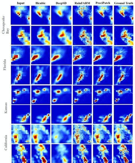
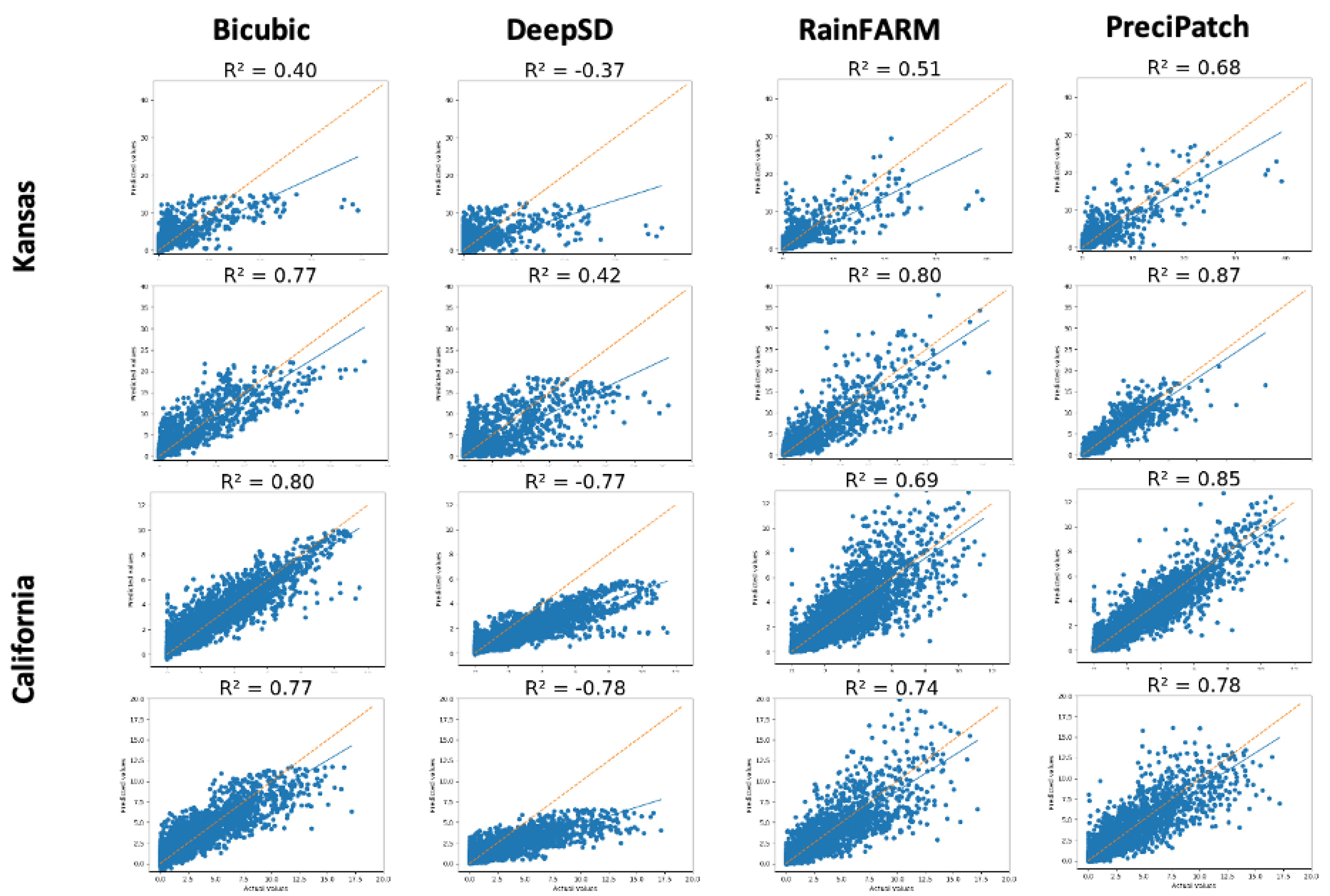
The methods used in downscaling case studies are chosen based on the ability to provide precipitation field as the final output and whether they require climate variables other than precipitation when producing downscaled results. Besides the statistical downscaling methods, bilinear interpolation (e.g., bicubic) is considered the baseline for spatial downscaling of precipitation fields [32]. Specifically, three methods are selected to evaluate besides the proposed method: (1) bicubic interpolation, (2) DeepSD, as an SRCNN based super-resolution downscaling method [36], and (3) RainFARM [28] as a stochastic downscaling method. Although there are other downscaling methods available in the research, most of them are not able to produce precipitation fields as output, require other datasets when downscaling, or they are limited to a specific area. Statistical methods like regression and PP methods are not chosen because they failed to produce continuous precipitation fields and require additional variables other than precipitation, which are not suitable for downscaling requirements in the previous section. Most of the statistical methods are involved using either observation data from the same time frame or other variables if precipitation field is desired as the downscaled result. Under this consideration, statistical methods are chosen.

3.2. Results

For each study area, two images from different time slices are selected to show a brief view of the general performance of the bicubic method, DeepSD, RainFARM, and PreciPatch. The original high-resolution IMERG data set is also visualized to compare with the downscaled results from different methods with a direct visual comparison. DeepSD is trained using the data from 2014 to 2017 at the same region, bicubic and RainFARM do not need a training process, and PreciPatch dictionary is trained using the whole U.S. coverage data from 2014 to 2017.

Figure 5 presents the downscaled results for different study areas. The input column in each figure contains the inputs for different downscaling methods and is used as the only input in downscale methods. The results from bicubic, DeepSD, RainFARM, and PreciPatch are in the next four columns, respectively. All the images from the same row share the same color scale. Original IMERG data are in the last column for visual comparison with different results. Generally, PreciPatch outperformed RainFARM, DeepSD, and bicubic, showing results closer to the ground truth in most cases. RainFARM method is a valid solution that meets downscaling requirements and can produce downscaling results with fast speed. However, due to the theoretical limitations of this method, which assumes rainfall fields as Gaussian random fields at all scale levels [27], the practical shapes and textures of rainfall are not sufficiently simulated by RainFARM. Bicubic is often treated as the baseline for downscaling, and the results from DeepSD are very close to those from bicubic. DeepSD is showing great potential for improvements.

3.3. Validation and Evaluation

The downscaled results are compared with ground truth statistically.

Figure 6 and Figure 7 show the direct comparison between the downscaled point values (predicted values) to the ground truth in the cases corresponding to the ones showing in Figure 5. Each plot represents a time slice. Statistically speaking, for R², bicubic and PreciPatch performs better than DeepSD and RainFARM in most cases. Six more criteria are used to evaluate the performance between different methods. A total of 2208 time slices (hourly precipitation from 2018 June, July, and August) are used from all four study regions to generate results. The statistical comparison is made through a grid-to-grid comparison between the predicted values from each method to the ground truth at each time slice. The detailed statistical comparison is shown in

Table 9. Statistical comparison.

mm/hour	Bicubic	DeepSD	RainFARM	PreciPatch
Average Bias per grid	0.03	0.12	4.3 × 10−9	0.003
Average R²	0.18	-0.16	0.29	0.42
Average (+) R²	0.44	0.3	0.47	0.57
RMSE	0.45	0.61	0.49	0.42
Mean Absolute Error	0.13	0.28	0.13	0.1
Maximum Absolute Error	7.75	7.95	4.2	3.87
STDV Absolute Error	0.2	0.27	0.09	0.07

; the values are averaged from all time slices, where PreciPatch shows the best statistical accuracies in almost all aspects, followed by RainFARM and bicubic. DeepSD has comparatively low performance in this case study, which agrees with the results from the pre-test and visual comparison. PreciPatch outperforms RainFARM, bicubic, and DeepSD in this synthetic experiment regarding statistical accuracy.

In addition to the visual and statistical comparison between methods, aggregation of the downscaled results was implemented to test the downscaling method’s ability to hold precipitation consistency from large-scale to small-scale. As designed with constrains for both RainFARM and PreciPatch, the downscaled results from these two methods could be upscaled to the original coarse-resolution input with visually unnoticeable variations. However, the downscaled results from bicubic interpolation and DeepSD methods could not be aggregated back to low-resolution inputs, which means such downscaling approaches represent a biased transformation from large-scale data to small-scale outputs.

3.4. Discussion

Major differences between our method and previous precipitation downscaling research include:

• Full-field generation instead of area limited generation or fixed size.
• Precipitation fields as target production instead of station networks (e.g., single or multiple), providing continuous information in 2D space.
• Precipitation field distribution simulated closer to precipitation observation
• Data independence in production (available for downscaling future predictions).
• Hourly precipitation downscaling to precipitation fields (downscaling short-duration precipitation events) instead of a daily average or seasonal downscaling used in other research.
• Using the prior knowledge learned in one data set and successfully applied to another related data set.
• The rainfall amount is consistent with large-scale vs. rainfall inconsistency in others.

Major differences between PreciPatch and other downscaling approaches regarding methodology includes: (1) comparing to statistical downscaling method: there is no need for other climate variables in the downscaling process, no regression process or probability assumption process, (2) comparing to stochastic downscaling method: the proposed method is making use of prior knowledge, not purely hypothesis and mathematical transformation based, (3) comparing to SRCNN based methods like DeepSD: when interpolation process is involved, the final output is constrained by coarse-resolution inputs, which is equal to an unbiased disaggregation of precipitation amounting to space, (4) comparing to traditional dictionary learning: one master dictionary is constructed instead of two in traditional approaches, the proposed method uses dynamic patches to recover the high-resolution image, while the traditional approach uses stored fixed patches, DTW distance is used instead of MSE or Euclidean distance, fuzzy search is utilized in the new method instead of exact search for similarity patches, and rainfall amount is consistent in the downscaled result, 5) comparing to Analog Method (AM): similarity searching is executed spatially with a fuzzy search instead of linearly with a direct search.

In this research, there are also some limitations to PreciPatch. For example, the computing time is longer than other downscaling methods, which makes it hard to apply to large datasets. The detailed comparison is in

Table 10. Comparison of tested downscaling method.

	Bicubic	DeepSD	RainFARM	PreciPatch
Training time	N/A	~1 hour for 3 months of data (national coverage)	N/A	~200 hours for 300 Million patches (national coverage)
Applicability to different areas?	Direct apply, no training is needed	Additional training is needed if the area is different or the input size is different	Direct apply, no training is needed	Direct apply, no need for additional training
Computing time	< 0.001 sec per grid point	~0.005 sec per grid point	~0.005 sec per grid point	~2 sec per grid point per process
Overall downscaling performance	Baseline	Not good—close to the baseline	Rainfall clusters are not well simulated	Best
Holds rainfall consistency with large-scale input?	No	No	Yes	Yes

.

However, this limitation could be resolved by including an additional index layer for the dictionary and reprogramming the system using more efficient languages such as C/C++. Another limitation for the proposed method is its assumption: future precipitation would behave similarly as its past, relationships developed for present climate also hold for possible future climates [39] (the same assumption is used in all statistical downscaling methods). One advantage compares with other models like DeepSD is that PreciPatch does not need additional training when applying to different areas, even for regions outside of the training area.

4. Conclusions

The importance of precipitation downscaling is well recognized in hydrological impact studies and local climate change-related domains. However, few statistical downscaling methods can provide universally applicable downscaling solutions for arbitrary GCM outputs, large amounts of precipitation downscaling related studies are area limited and highly additional data-dependent, not applicable for random locations. Meanwhile, major research can only provide the downscaled result on a level of single or multiple stations. Providing precipitation fields as outputs are still beyond the reach for most traditional methods. Recent developments in the stochastic downscaling method and the SR based method brought new opportunities to enhance downscaling studies. A new precipitation downscaling method based on dynamic dictionary learning is proposed with detailed algorithms and procedures. Four precipitation downscaling study cases are conducted to evaluate the performance of the proposed method and compare it with other downscaling methods (RainFARM and DeepSD), along with the comparison baseline, the bicubic interpolation method. Results from case studies have shown positive feedback on the proposed downscaling method, demonstrating good quality for simulating spatially distributed precipitation fields and yielding the best performance among all other tested methods through visual inspection and quantitative analyses. It is hard for traditional and machine learning super-resolution based methods to exclude the interpolation process and include the non-linear characteristics of precipitation event into the method design [41]. Meanwhile, many downscaling methods like bicubic interpolation and DeepSD do not have extra constraints to enforce the final outputs to hold rainfall consistency with the initial inputs. The proposed method interprets the downscaling task as a constrained single image super-resolution problem, different from traditional approaches and other downscaling methods, it addresses the precipitation downscaling issue using a novel approach which excludes the interpolation process and is able to generate non-linear spatial patterns that are closer to rainfall observations. Additionally, rainfall consistency is ensured by adding extra constraints in the proposed method. As a result, PreciPatch achieved better results than other downscaling methods in precipitation downscaling study cases because it takes the spatial characteristics of precipitation into the method design consideration and optimizes the method to fit precisely for the precipitation downscaling scenario.

Precipitation field downscaling is a challenging task, and related research topics have been explored by many studies. The proposed precipitation downscaling method, PreciPatch has shown its ability to spatially downscale short-duration precipitation events to precipitation fields and can be applied to downscale future estimations from GCMs or other gridded data sources. The bias correction is not addressed by PreciPatch, and the bias from GCMs are preserved at the same spatial scale as the input. This research contributes to hydrological impact studies and local climate change studies by providing a precipitation downscaling method and associated algorithms for simulating precipitation fields in local scale and being consistent with large-scale information, in detail:

• This method does not require additional data as predictors to produce downscaled results, and it could be used for downscaling future estimations from GCMs.
• This downscaling method has the potential to aid climate models like WRF by providing higher resolution inputs.
• The downscaled results from this method could be used to force mountain glacier models for local impact studies, where the complete absence of climate monitoring activities within the regions of interest presents a data challenge.

For future work, more (spatiotemporal) indexing techniques [42] will be integrated to accelerate the similarity search process in PreciPatch. PreciPatch will be converted and rebuilt on top of a machine learning framework to generalize the dictionary into a model, accelerate the downscaling process, and reduce storage requirement. More observation data will be used to evaluate the downscaling method regarding expandability and transferability.

References

1. Sheehan, M.C.; Fox, M.A.; Kaye, C.; Resnick, B. Integrating health into local climate response: Lessons from the US CDC Climate-Ready States and cities initiative. Environ. Health Perspect. 2017, 125, 094501. [Google Scholar] [CrossRef] [Green Version]
2. Fatichi, S.; Ivanov, V.Y.; Caporali, E. Assessment of a stochastic downscaling methodology in generating an ensemble of hourly future climate time series. Clim. Dyn. 2013, 40, 1841–1861. [Google Scholar] [CrossRef] [Green Version]
3. Yang, C.; Yu, M.; Li, Y.; Hu, F.; Jiang, Y.; Liu, Q.; Sha, D.; Xu, M.; Gu, J. Big Earth data analytics: A survey. Big Earth Data 2019, 3, 83–107. [Google Scholar] [CrossRef] [Green Version]
4. Climate.gov, n.d. Climate Models|NOAA Climate.gov. Available online: https://www.climate.gov/maps-data/primer/climate-models (accessed on 24 August 2019).
5. Benestad, R. Downscaling Climate Information. Oxford Research Encyclopedia of Climate Science. 2016. Available online: https://oxfordre.com/climatescience/view/10.1093/acrefore/9780190228620.001.0001/acrefore-9780190228620-e-27 (accessed on 24 August 2019).
6. Giorgi, F.; Mearns, L.O. Approaches to regional climate change simulation: A review. Rev. Geophys 1991, 29, 1–2. [Google Scholar] [CrossRef]
7. Arritt, R.W.; Rummukainen, M. Challenges in regional-scale climate modeling. Bull. Am. Meteorol. Soc. 2011, 92, 365–368. [Google Scholar] [CrossRef] [Green Version]
8. Walton, D.B.; Sun, F.; Hall, A.; Capps, S. A hybrid dynamical–statistical downscaling technique. Part I: Development and validation of the technique. J. Clim. 2015, 28, 4597–4617. [Google Scholar] [CrossRef]
9. Wilby, R.L. Statistical downscaling of daily precipitation using daily airflow and seasonal teleconnection indices. Clim. Res. 1998, 10, 163–178. [Google Scholar] [CrossRef]
10. Maraun, D.; Wetterhall, F.; Ireson, A.M.; Chandler, R.E.; Kendon, E.J.; Widmann, M.; Brienen, S.; Rust, H.W.; Sauter, T.; Themeßl, M.; et al. Precipitation downscaling under climate change: Recent developments to bridge the gap between dynamical models and the end user. Rev. Geophys. 2010, 48. [Google Scholar] [CrossRef]
11. Xu, C.Y. Climate change and hydrologic models: A review of existing gaps and recent research developments. Water Resour. Manag. 1999, 13, 369–382. [Google Scholar] [CrossRef]
12. Bronstert, A.; Kolokotronis, V.; Schwandt, D.; Straub, H. Comparison and evaluation of regional climate scenarios for hydrological impact analysis: General scheme and application example. Int. J. Climatol. A J. R. Meteorol. Soc. 2007, 27, 1579–1594. [Google Scholar] [CrossRef]
13. Rau, M.; He, Y.; Goodess, C.; Bárdossy, A. Statistical downscaling to project extreme hourly precipitation over the United Kingdom. Int. J. Climatol. 2019, 40, 1805–1823. [Google Scholar] [CrossRef]
14. Kundzewicz, Z.W.; Mata, L.J.; Arnell, N.W.; Doll, P.; Kabat, P.; Jimenez, B.; Miller, K.; Oki, T.; Zekai, S.; Shiklomanov, I. Freshwater Resources and Their Management; Parry, M.L., Canziani, O.F., Palutikof, J.P., van der Linden, P.J., Hanson, C.E., Eds.; Climate Change 2007: Impacts, Adaptation and Vulnerability. Contribution of Working Group II to the Fourth Assessment Report of the Intergovernmental Panel on Climate Change; Cambridge University Press: Cambridge, UK, 2007; pp. 173–210. ISBN 9780521880091. [Google Scholar]
15. Vrac, M.; Naveau, P. Stochastic downscaling of precipitation: From dry events to heavy rainfalls. Water Resour. Res. 2007, 43, 7. [Google Scholar] [CrossRef] [Green Version]
16. Vandal, T.J. Statistical Downscaling of Global Climate Models with Image Super-resolution and Uncertainty Quantification. Ph.D Thesis, Northeastern University, Boston, MA, USA, 2018. [Google Scholar]
17. Lenderink, G.; Van Meijgaard, E. Increase in hourly precipitation extremes beyond expectations from temperature changes. Nat. Geosci. 2008, 1, 511. [Google Scholar] [CrossRef]
18. Wilks, D.S. Use of stochastic weather generators for precipitation downscaling. Wiley Interdiscip. Rev. Clim. Chang. 2010, 1, 898–907. [Google Scholar]
19. Wilby, R.L.; Wigley, T.M.L. Downscaling general circulation model output: A review of methods and limitations. Prog. Phys. Geogr. 1997, 21, 530–548. [Google Scholar] [CrossRef]
20. Wilby, R.L.; Charles, S.P.; Zorita, E.; Timbal, B.; Whetton, P.; Mearns, L.O. Guidelines for use of climate scenarios developed from statistical downscaling methods. In Supporting Material of the Intergovernmental Panel on Climate Change; DDC of IPCC TGCIA: Geneva, Switzerland, 2004. [Google Scholar]
21. Fowler, H.J.; Blenkinsop, S.; Tebaldi, C. Linking climate change modelling to impacts studies: Recent advances in downscaling techniques for hydrological modelling. Int. J. Climatol. A J. R. Meteorol. Soc. 2007, 27, 1547–1578. [Google Scholar] [CrossRef]
22. Tang, J.; Niu, X.; Wang, S.; Gao, H.; Wang, X.; Wu, J. Statistical downscaling and dynamical downscaling of regional climate in China: Present climate evaluations and future climate projections. J. Geophys. Res. Atmos. 2016, 121, 2110–2129. [Google Scholar] [CrossRef] [Green Version]
23. Wang, Y.Q.; Leung, L.R.; McGregor, J.L.; Lee, D.K.; Wang, W.C.; Ding, Y.H.; Kimura, F. Regional climate modeling: Progress, challenges, and prospects. J. Meteorol. Soc. Jpn. 2004, 82, 1599–1628. [Google Scholar] [CrossRef] [Green Version]
24. Chen, J.; Brissette, F.P.; Leconte, R. Coupling statistical and dynamical methods for spatial downscaling of precipitation. Clim. Chang. 2012, 114, 509–526. [Google Scholar] [CrossRef]
25. Jarosch, A.H.; Anslow, F.S.; Clarke, G.K. High-resolution precipitation and temperature downscaling for glacier models. Clim. Dyn. 2012, 38, 391–409. [Google Scholar] [CrossRef]
26. Chen, J.; Chen, H.; Guo, S. Multi-site precipitation downscaling using a stochastic weather generator. Clim. Dyn. 2018, 50, 1975–1992. [Google Scholar] [CrossRef]
27. Liu, Q.; Li, Y.; Yu, M.; Chiu, L.S.; Hao, X.; Duffy, D.Q.; Yang, C. Daytime Rainy Cloud Detection and Convective Precipitation Delineation Based on a Deep Neural Network Method Using GOES-R ABI Images. Remote Sens. 2019, 11, 2555. [Google Scholar] [CrossRef] [Green Version]
28. Rebora, N.; Ferraris, L.; von Hardenberg, J.; Provenzale, A. RainFARM: Rainfall downscaling by a filtered autoregressive model. J. Hydrometeorol. 2006, 7, 724–738. [Google Scholar] [CrossRef]
29. Posadas, A.; Duffaut Espinosa, L.A.; Yarlequé, C.; Carbajal, M.; Heidinger, H.; Carvalho, L.; Jones, C.; Quiroz, R. Spatial random downscaling of rainfall signals in Andean heterogeneous terrain. Nonlinear Process. Geophys. 2015, 22, 383–402. [Google Scholar] [CrossRef] [Green Version]
30. Terzago, S.; Palazzi, E.; Hardenberg, J.V. Stochastic downscaling of precipitation in complex orography: A simple method to reproduce a realistic fine-scale climatology. Nat. Hazards Earth Syst. Sci. 2018, 18, 2825–2840. [Google Scholar] [CrossRef] [Green Version]
31. He, X.; Chaney, N.W.; Schleiss, M.; Sheffield, J. Spatial downscaling of precipitation using adaptable random forests. Water Resour. Res. 2016, 52, 8217–8237. [Google Scholar] [CrossRef]
32. Dong, C.; Loy, C.C.; He, K.; Tang, X. Learning a deep convolutional network for image super-resolution. In Proceedings of the European conference on computer vision, Zurich, Switzerland, 6–12 September 2014; pp. 184–199. [Google Scholar]
33. Kim, J.; Kwon Lee, J.; Mu Lee, K. Accurate image super-resolution using very deep convolutional networks. In Proceedings of the IEEE conference on computer vision and pattern recognition, Las Vegas, NV, USA, 27–30 June 2016; pp. 1646–1654. [Google Scholar]
34. Zhang, Y.; Li, K.; Li, K.; Wang, L.; Zhong, B.; Fu, Y. Image super-resolution using very deep residual channel attention networks. In Proceedings of the European Conference on Computer Vision (ECCV), Munich, Germany, 8–14 September 2018; pp. 286–301. [Google Scholar]
35. Ebtehaj, A.M.; Foufoula-Georgiou, E.; Lerman, G. Sparse regularization for precipitation downscaling. J. Geophys. Res. Atmos. 2012, 117. [Google Scholar] [CrossRef] [Green Version]
36. Vandal, T.; Kodra, E.; Ganguly, S.; Michaelis, A.; Nemani, R.; Ganguly, R.A. Deepsd: Generating high resolution climate change projections through single image super-resolution. In Proceedings of the 23rd Acm Sigkdd International Conference on Knowledge Discovery and Data Mining, ACM, Halifax, NS, Canada, 13–17 August 2017; pp. 1663–1672. [Google Scholar]
37. Freeman, W.T.; Jones, T.R.; Pasztor, E.C. Example-based super-resolution. IEEE Comput. Graph. Appl. 2002, 22, 56–65. [Google Scholar] [CrossRef] [Green Version]
38. Itakura, F. Minimum prediction residual principle applied to speech recognition. IEEE Trans. Acoust. Speech Signal Process. 1975, 23, 67–72. [Google Scholar] [CrossRef]
39. Keogh, E.; Ratanamahatana, C.A. Exact indexing of dynamic time warping. Knowl. Inf. Syst. 2005, 7, 358–386. [Google Scholar] [CrossRef]
40. Tan, C.W.; Webb, G.I.; Petitjean, F. Indexing and classifying gigabytes of time series under time warping. In Proceedings of the 2017 SIAM international Conference on Data Mining. Society for Industrial and Applied Mathematics, Houston, TX, USA, 27–29 April 2017; pp. 282–290. [Google Scholar]
41. Yu, M.; Bambacus, M.; Cervone, G.; Clarke, K.; Duffy, D.; Huang, Q.; Li, J.; Li, W.; Li, Z.; Liu, Q.; et al. Spatiotemporal event detection: A review. Int. J. Digit. Earth 2020. [Google Scholar] [CrossRef] [Green Version]
42. Yang, C.; Clarke, K.; Shekhar, S.; Tao, C.V. Big Spatiotemporal Data Analytics: A research and innovation frontier. Int. J. Geogr. Inf. Sci. 2019, 1–14. [Google Scholar] [CrossRef] [Green Version]
Figure 1. PreciPatch method workflow.
Remotesensing 12 01030 g001
Figure 2. A graph representation of Diff Array.
Remotesensing 12 01030 g002
Figure 3. Dictionary classification.
Remotesensing 12 01030 g003
Figure 4. Study areas for downscaling studies.
Remotesensing 12 01030 g004
Figure 5. Downscaling results. The x-axis refers to the longitude, and the y-axis refers to the latitude. Each row is the input aggregated Integrated Multi-satellitE Retrievals for GPM (IMERG) rain rate, Bicubic result, DeepSD result, RainFARM result, PreciPatch result and original high-resolution IMERG rain rate respectively for each location. 1st row: hourly precipitation at Chesapeake Bay area on 2018/7/21 (23:30:00 UTC), 2nd row: hourly precipitation at Chesapeake Bay area on 2018/7/21 (16:30:00 UTC), 3rd row: hourly precipitation at Florida area on 2018/12/14 (05:30:00 UTC), 4th row: hourly precipitation at Florida area on 2018/12/14 (18:30:00 UTC), 5th row: hourly precipitation at Kansas area on 2018/7/29 (04:30:00 UTC), 6th row: hourly precipitation at Kansas area on 2018/7/29 (08:30:00 UTC), 7th row: hourly precipitation at California area on 2018/1/9 (00:30:00 UTC), 8th row: hourly precipitation at California area on 2018/1/9 (08:30:00 UTC).
Remotesensing 12 01030 g005
Figure 6. The Chesapeake Bay and Florida—R². The x-axis refers to the ground truth, and the y-axis is the prediction. The 45 degrees line in each graph is the perfect match reference line between the prediction and the ground truth, showing as the dashed line, the solid line is the trending line. 1st row: hourly precipitation at Chesapeake Bay area on 2018/7/21 (23:30:00 UTC), 2nd row: hourly precipitation at Chesapeake Bay area on 2018/7/21 (16:30:00 UTC), 3rd row: hourly precipitation at Florida area on 2018/12/14 (05:30:00 UTC), 4th row: hourly precipitation at Florida area on 2018/12/14 (18:30:00 UTC).
Remotesensing 12 01030 g006
Figure 7. Kansas and California—R². The x-axis refers to the ground truth, and the y-axis is the prediction. The 45 degrees line in each graph is the perfect match reference line between the prediction and the ground truth, showing as the dashed line, the solid line is the trending line. 1st row: hourly precipitation at Kansas area on 2018/7/29 (04:30:00 UTC), 2nd row: hourly precipitation at Kansas area on 2018/7/29 (08:30:00 UTC), 3rd row: hourly precipitation at California area on 2018/1/9 (00:30:00 UTC), 4th row: hourly precipitation at California area on 2018/1/9 (08:30:00 UTC).
Remotesensing 12 01030 g007