Article

Hyperspectral and Multispectral Remote Sensing Image Fusion Based on Endmember Spatial Information

1
State Key Laboratory of Information Engineering in Surveying, Mapping, and Remote Sensing, Wuhan University, Wuhan 430079, China
2
School of Electronics Information and Communications, Huazhong University of Science and Technology, 1037 Luoyu Road, Wuhan 430074, China
3
School of Computer Science, Wuhan University, Wuhan 430072, China
4
Hongyi Honor College, Wuhan University, Wuhan 430072, China
*
Author to whom correspondence should be addressed.
Remote Sens. 2020, 12(6), 1009; https://doi.org/10.3390/rs12061009
Submission received: 12 February 2020 / Revised: 14 March 2020 / Accepted: 15 March 2020 / Published: 21 March 2020
(This article belongs to the Section Remote Sensing Image Processing)

Abstract

:
Hyperspectral (HS) images usually have high spectral resolution and low spatial resolution (LSR). However, multispectral (MS) images have high spatial resolution (HSR) and low spectral resolution. HS–MS image fusion technology can combine both advantages, which is beneficial for accurate feature classification. Nevertheless, heterogeneous sensors always have temporal differences between LSR-HS and HSR-MS images in the real cases, which means that the classical fusion methods cannot get effective results. For this problem, we present a fusion method via spectral unmixing and image mask. Considering the difference between the two images, we firstly extracted the endmembers and their corresponding positions from the invariant regions of LSR-HS images. Then we can get the endmembers of HSR-MS images based on the theory that HSR-MS images and LSR-HS images are the spectral and spatial degradation from HSR-HS images, respectively. The fusion image is obtained by two result matrices. Series experimental results on simulated and real datasets substantiated the effectiveness of our method both quantitatively and visually.

1. Introduction

Hyperspectral (HS) images are playing important roles in agriculture, medical science, remote sensing, and other fields because of its high spectral resolution [1]. The spectrum width of hyperspectral sensor is narrow, resulting in insufficient energy. In order to maintain a certain signal-to-noise ratio (SNR), the spatial resolution has to be sacrificed. Therefore, multispectral (MS) images often have higher spatial resolution than HS images. High spatial resolution (HSR) information helps to obtain more accurate locations and shapes of ground objects [2], and spectral information helps to identify types of features from images [3]. Spectral information fusion of HS images and MS images is helpful for image retrieval [4], classification [5,6], image analysis [7,8] and information extraction [2,9]. Fusing low spatial resolution HS (LSR-HS) images and HSR-MS images can obtain HSR-HS images [10], which is very helpful for fine mapping, ground objects identification, and so on.
Pansharpening is a special case of HS–MS images fusion problem [11], which enhances the spatial resolution of LSR-MS image by fusing it with the panchromatic image [12]. With the development of hyperspectral imaging technology, these methods are gradually applied to hyperspectral images [13]. For instance, component substitution (CS)-based methods convert the LSR-HS image to another orthogonal space and replace the decomposed spatial components with one of the multispectral bands [14,15], including Gram–Schmidt adaptive (GSA) [16]. Another representative pansharpening method is multi-resolution analysis (MRA), which utilizes the multiresolution decomposition way to obtain the spatial information of panchromatic image and combine it into the resampled HS bands. The well-known methods include generalized Laplacian pyramid (GLP) [17].
Another kind of HS–MS fusion method is to take HSR-MS image and LSR-HS image as degradation results of HSR-HS image in spectrum and space, respectively, and then inversing two images to reconstruct the target image. This category method mainly includes the Bayesian-based method and spectral unmixing-based method. The Bayesian-based method uses the posterior probability distribution of the target image for image fusion given LSR-HS and HSR-MS images [18,19,20]. For instance, Eismann et al. proposed a Bayesian-based method under the maximum a posteriori (MAP) estimation, which estimated the underlying spectral characteristics of the ground objects by a stochastic mixing model (SMM) and optimized the estimated HS images relative to the input images by a cost function [21].
The spectral unmixing-based fusion method has been widely studied because of its physically straightforward representation of the fusion process. Each pixel is a mixture of some endmember spectra and corresponding fractional abundances [22]. The approach based on spectral unmixing is obtaining endmember matrix and abundance matrix from LSR-HS image and HSR-MS image using spectral mixture model, respectively. Then, two resulting matrices are reconstructed as the HSR-HS image. For instance, coupled nonnegative matrix factorization (CNMF) [23] alternately using NMF unmixing the LSR-HS image and HSR-MS image to get the endmember and abundance matrices, respectively. A method proposed by Akhtar et al. [24] is to extract the endmember spectra as a spectral basis first, and then with the basis fixed use a pursuit method reconstruct the image. The method proposed by Lanaras et al. [25] is to obtain the endmembers by alternately updating method and use the projection gradient method to get abundance matrix of HSR-MS image.
Most HS–MS fusion methods require a high correlation between LSR-HS images and HSR-MS images. The correlation between the two images is affected by various factors such as sensor characteristics, temporal difference, weather, imaging angle, etc., and the real data is often difficult to meet the requirements [25]. To solve the problem, we propose a new HS–MS fusion method based on linear spectral mixture model (LSMM), which investigates the endmember signatures’ spatial relationship between LSR-HS image and HSR-MS image. First, in order to ensure the consistency of the endmembers positions in two images, the mask is generated according to the differences between the two images. Then, the proposed method eliminates the variation area by masking the large difference regions. After that, we extract the endmembers and their corresponding positions from masked LSR-HS image and locate them according to the endmember spatial information in HSR-MS image. Next, based on the obtained endmember matrix, the abundance matrix is calculated by nonnegative linear regression. Finally, the HSR-HS image is reconstructed by endmember matrix of LSR-HS image and abundance matrix of HSR-MS image. Our fusion method is physical clear and has very simple model with less calculation, and it is robust to the image temporal difference. Experimental results based on the simulated images and real images indicate our method can effectively integrate the spatial and spectral information, and outperform than other compared methods.

2. Methodology

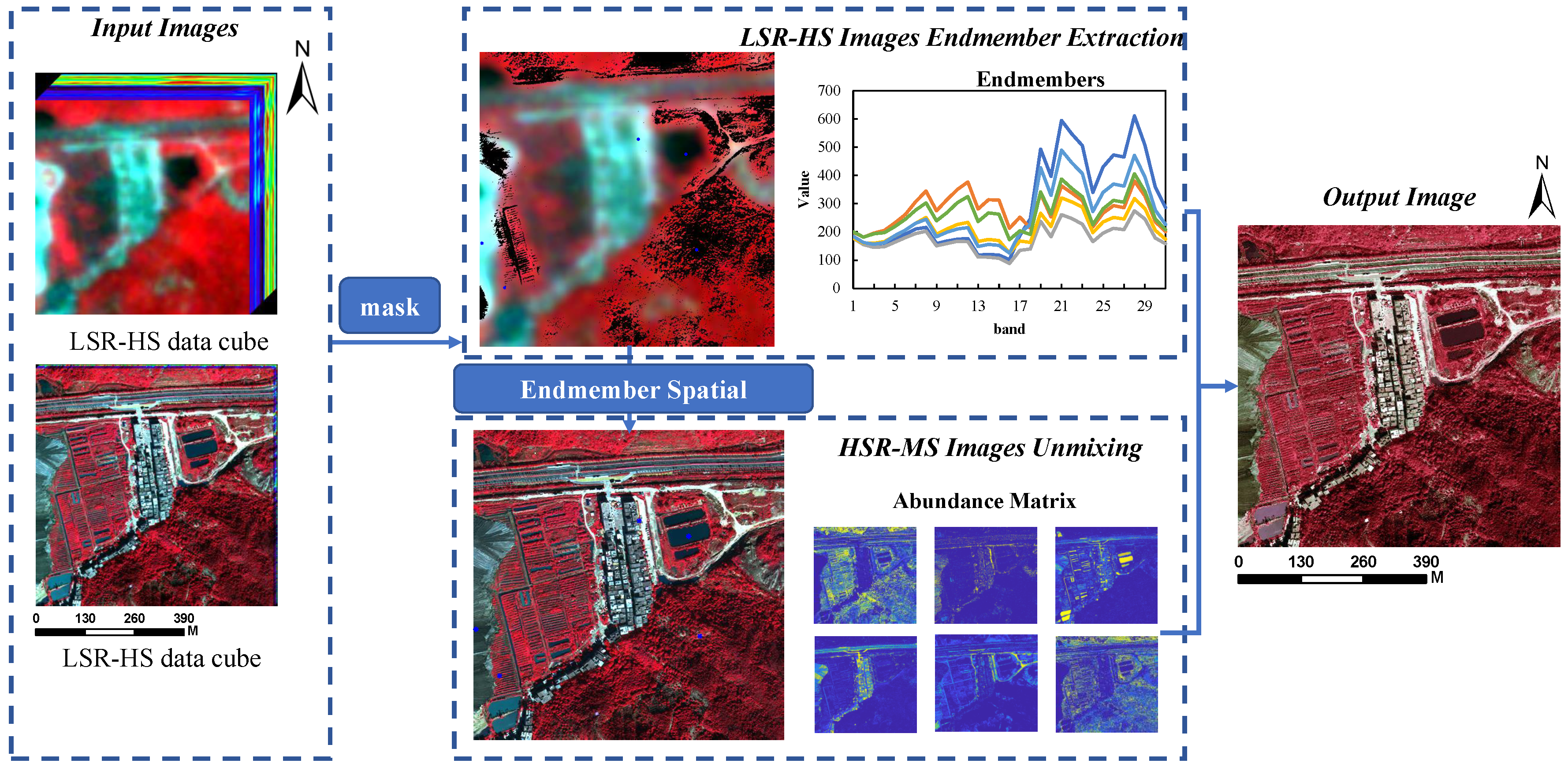
2.1. The Proposed Method Overview

LSMM is widely used to represent the observation images because of its effectiveness and straightforward [22]. The LSMM considers the ground to be flat and assumes that incoming sunlight radiation is reflected off the surface only in a single reflection, not multiple scattering [26]. Each pixel in the scene can be modeled as a linear combination of all the spectra of the materials and the proportional contribution of each spectra. Let X = x 1 , , x N L × N denotes the observation image, L is the number of bands, N is the number of all pixels. For the j-th pixel, x j = x 1 j , , x L j T L , the LSMM models the pixel as:
x j = i = 1 P s i , j a i + n j = A s j + n j
where A = a 1 , , a P L × P is the mixing matrix that consists of P distinct endmember spectral signiatures, P is the number of endmember signatures in the scene, s j = s 1 j , , s P j T P is the abundance vector of x j , and n j L is the additive noise term. Because of the physical constraints, the abundance is nonnegtive s i j 0 and sum-to-one i = 1 P s i j = 1 . Correspondingly, the image has N pixels can be modeled as:
X = AS + N
Based on LSMM, the LSR-HS image X h and HSR-MS image X m can be modeled as:
X m = A m S m + N m X h = A h S h + N h
where A m L m × P is the endmember matrix of HSR-MS image X m , L m is the band number, P is the endmember number. S m P × N m denotes the abundance matrix, N m denotes the number of pixels. N m L m × N m denotes the additive noise term. For LSR-HS image X h , A h L h × P is the endmember matrix, and L h is the band number. S h P × N h is the abundance matrix of X h , N h is the number of pixels. N h L h × N h is the noise term of LSR-HS image. If we upsample the LSR-HS image to the same size as the HSR-MS image, the number of pixels will be the same N m = N h = N . Based on the physical meaning of abundance matrix and endmember matrix, all the matrices in Equation (3) are nonnegative.
Under the assumption that HSR-MS image and LSR-HS image is the spectral and spatial degradation from HSR-HS image, respectively. We assume that A m and A h denote the same endmember signatures, and the difference between them is only in the spectral resolution. In this way, HSR-HS image Z can be expressed as:
Z A h S m
where Z L h × N has N pixels with L h bands. A h and S m provides the spectral information and spatial information for Z , respectively.
From Equation (4), we can see that the key of HS–MS fusion based on spectral unmixing is how to ensure A m and A h are the same endmembers. Many methods assume that HSR-MS image and LSR-HS image are obtained from spatial and spectral degradation of HSR-HS image, respectively [27]. For this reason, we propose a HS–MS fusion method based on endmember spatial information and regional mask. Figure 1 shows the overall flowchart of the proposed method. This method consists of three main parts: regional mask, LSR-HS image unmixing and HSR-MS image unmixing.
Since it is difficult to obtain the simultaneous LSR-HS image and HSR-MS image of the same area in the real case, our method proposes a regional mask prepossessing based on the ground objects variation caused by temporal difference. The method masks the areas with large differences between two images and extracts the endmembers from areas with small changes. In this way, endmembers of the fusion part from two images are consistent. This part will be described in detail in Section 2.2.
In this paper, the proposed fusion method is based on the spectral unmixing model, and the most classical and practical endmember extraction method Vertex Component Analysis (VCA) [28] is used to obtain the LSR-HS image endmember signatures. Based on the convex geometry theory, the endmember spectra and corresponding positions of the pure pixels can be obtained by VCA. This part will be described in detail in Section 2.3.
Based on the principle of one-to-one match between LSR-HS image and HSR-MS image endmember positions, we can obtain the pure pixels’ positions in HSR-MS image from LSR-HS image endmember positions. Since LSR-HS image can be regarded as the spatial downsampling result of HSR-MS image, the pixels’ mean value of the region is selected as the HSR-MS endmember results. We take the endmembers’ pixels positions of LSR-HS image as the center of the region and the resolution ratio of the two images as the diameter. Then, according to LSMM model and HSR-MS endmemebr matrix, the corresponding abundance matrix is obtained by using nonnegative constrained least squares (NCLS) [29]. This part will be described in detail in Section 2.4.
After obtaining A h and S m from LSR-HS image X h and HSR-MS image X m , respectively, we reconstruct the HSR-HS image Z ^ according to Equation (4).

2.2. Regional Mask of the LSR-HS Image and HSR-HS Image Variation Area

Under the premise of accurate registration, the image position and actual position of the two images should correspond to each other. Due to the temporal difference, two images must have some variation regions. Therefore, this paper uses the regional mask caused by temporal difference to preprocess the image, which can eliminate the difference between LSR-HS and HSR-MS images.
Firstly, according to the band wavelength of Landsat8 (Blue: 450–515 nm, Green: 525–600 nm, Red: 630–680 nm, Near infrared (NIR): 845–885 nm), select the bands in the corresponding wavelength range in X h , and obtain four matrices as the spectral patches, Blue band patches: X h B = X h B 1 , , X h B n , Green band patches: X h G = X h G 1 , , X h G n , Red band patches: X h R = X h R 1 , , X h R n and NIR band patches: X h N I R = X h N I R 1 , , X h N I R n . We integrate four spectral patches and simulate a new LSR-MS image X h = [ X ¯ h B , X ¯ h G , X ¯ h R , X ¯ h N I R ] L m × N with four bands by averaging X h B , X h G , X h R , X h N I R , respectively.
Then, HSR-MS image X m and simulated LSR-MS image X h are normalized separately to eliminate the spectral difference. Since the near infrared band is sensitive to vegetation information, we make a subtraction between of the two images on the near infrared band to obtain regions with variation. We assume that if the results larger than t h r e s h 1 , the features in this region vary greatly, so we take this area as the mask region, defined as Equation (5).
M i , j = 1 , i f X i , j X i , j t h r e s h 1 0 , else
X h m a s k = X h · M
X m m a s k = X m · M
After determine the mask matrix M , we can get masked HSR-HS image X h m a s k and LSR-MS image X m m a s k images via Equations (6) and (7), respectively. In X h m a s k and X m m a s k , we assume that the ground objects are consistent in species and positions. In this paper, we focus on the spectrum of vegetation, rather than specific plants. So, we use mask without considering the vegetation types, or seasonal changes.

2.3. LSR-HS Image Endmember Extracting

Hyperspectral images can be modeled as a collection of spectral signatures, called endmembers. We use the commonly used VCA [28] to extract endmembers, becuase its accuracy is higher and it is easy to implement.
Generally, the HSIs unmixing problem based on LSMM is solved by using the square Frobenius norm of residual matrix as the cost function [30]. We use Equation (8) to extract endmembers from the LSR-HS image.
min A h , S h X h m a s k A h S h F 2 subject to A h 0 , S h 0
where · F 2 indicates the Frobenius norm. Because of the physical constraints of endmember matrix and abundance matrix, both of them should be non-negative. According to the convex geometry characteristic of HSIs, hyperspectral points cloud will be located in the simplex after affine transformation. The mixed pixels are locate interior the simplex and the endmembers are locate in the vertex of the simplex. VCA algorithm utilizes the geometric characteristic of HSIs and extracts endmembers by finding the pure pixels locate at the vertices of the simplex, which maximize the volume of the simplex and include all pixels. In this paper, we obtain the endmembers A h and corresponding positions P h from the masked LSR-HS image X h m a s k by VCA. All the endmembers are used to model the pixels in the dataset.

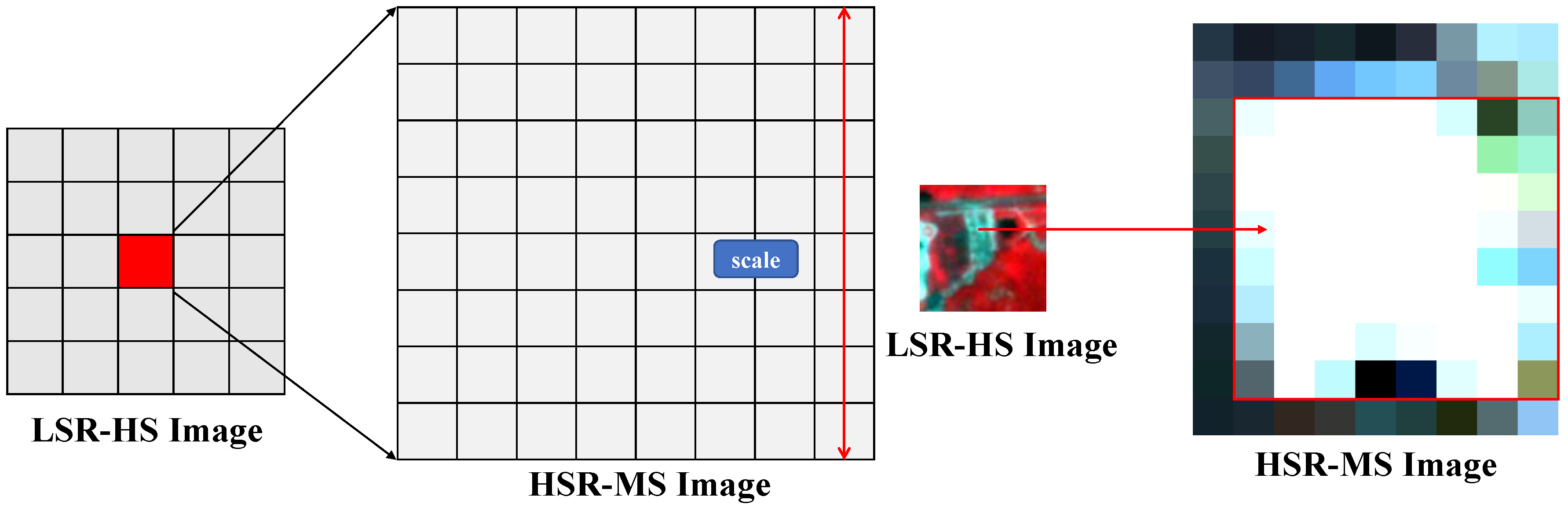
2.4. HSR-MS Image Unmixing

LSR-HS image can be regarded as the spatial downsampling result of LSR-HS image, in this way, the locations of pure pixels in LSR-HS image, corresponding to a region in HSR-MS image [31]. In terms of spectral information, LSR-HS image has a higher spectral resolution and a larger number of bands, HSR-MS image can be regarded as the spectral downsampling result of LSR-HS image [27]. Therefore, we assume that the pixels of this region in HSR-MS image constitutes the corresponding pure pixels in LSR-HS image.
In this paper, the spectral information of LSR-HS image and spatial information of HSR-MS image are combined for HSR-HS image fusion. According to endmember positions P h in LSR-HS image, we can get the pixel position of each endmember in HSR-MS image (as shown in Figure 2). We take this position as the center point, s c a l e as the diameter to get the corresponding endmember region P m . The size of each endmember region in HSR-MS image is s c a l e × s c a l e . Then, by averaging the pixels in the corresponding region, the result is taken as the endmember of the HSR-MS image.
However, in the real case, each endmember corresponding region in HSR-MS image may have more than one kind of ground objects. To solve this problem, we use spectral angle distance d to eliminate the different pixels in the region, which defined in Equation (9).
d = cos 1 x m i 1 , j 1 x m i 2 , j 2 x m i 1 , j 1 x m i 2 , j 2
where x m i 1 , j 1 and x m i 2 , j 2 denote the pixels in the region. We calculate the distance between each pixel in the region, select the pixels with closer distance value and take their mean value as the endmember A m of HSR-MS image. In addition, in order to avoid the second type of objects in the region, we sort them according to the distance between pixels, and select the first 90% as the candidate pixels.
After obtaining the endmember matrix A m of HSR-MS image, the corresponding abundance matrix S m can be calculated by Equation (10).
min S m X m A m S m F 2 subject to S m 0
According to Equation (10), we obtain the abundance matrix S m of HSR-MS image by nonnegative constrained least-squares (NCLS) algorithm.

3. Experiments and Results

In order to test the effectiveness of our method, we design the experiments by Wald’s protocol [13]. Then, the proposed method and other six fusion methods, including CNMF [23], fast fusion based on Sylvester equation (FUSE) [18], GLP [17], GSA [16], HS Superresolution (HySure) [20] and MAPSMM [21] are used to fuse and compare the results (The comparative methods’ codes are download from http://naotoyokoya.com/Download.html). Here, Z denotes the HSR-HS image as the reference image, and Z ^ denotes the fused image as the estimated HSR-HS image. Some popular metrics are used to evaluate the fused results, Peak-SNR, Spectral Angle Mapper (SAM) [32], Erreur Relative Globale Adimensionnelle de synthèse (ERGAS) [33] and Q2n.

3.1. Performance Evaluation Metrics

  • PSNR
    PSNR is for measuring the spatial quality of each band. It is the ratio between the maximum pixel value and the mean square error of the reconstructed image in each band. The PSNR of the i-th band is defined as:
    PSNR z i , z ^ i = 10 · log 10 max z i 2 z i z ^ i 2 2 z i z ^ i 2 2 N N
    where max z ^ i is the maximum pixel value in the i th band of the reference image, N is the pixel number of z ^ .
  • SAM
    SAM [32] is for quantifying the spectral similarity between the estimated and reference spectra in each pixel. The smaller of the SAM value indicates the higher spectral quality, the smaller spectral distortion.
    SAM = 1 L h arccos z ^ i T z i z i 2 z ^ i 2
    where · 2 denotes the l 2 norm.
  • ERGAS
    EGRAS index [33] describes the global statistical quality of the fused data, the smaller the better.
    ERGAS = 100 S 1 N i = 1 N Z ^ i Z i 2 2 1 L i = 1 L Z i 2
    where S is the ground sampling distance (GSD) ratio between the HSR-MS and LSR-HS images.
  • Q2n
    Q2n is a generalization of the universal image quality index (UIQI) [34] to measure the spatial and spectral quality in monochromatic images. The UIQI between reference image Z and fused image Z ^ is defined as:
    Q 2 n = 4 σ z ^ , z ^ ¯ z · z ¯ σ z ^ 2 + σ z 2 ^ ¯ z 2 + z ¯ 2
    where ^ ¯ z = 1 N i = 1 N z ^ i , z ¯ = 1 N i = 1 N z i , σ z = 1 N i = 1 N z i z ¯ 2 , σ z ^ = 1 N i = 1 N z ^ i ^ ¯ z 2 , σ z ^ , z = 1 N i = 1 N z ^ i ^ ¯ z z i z ¯ .

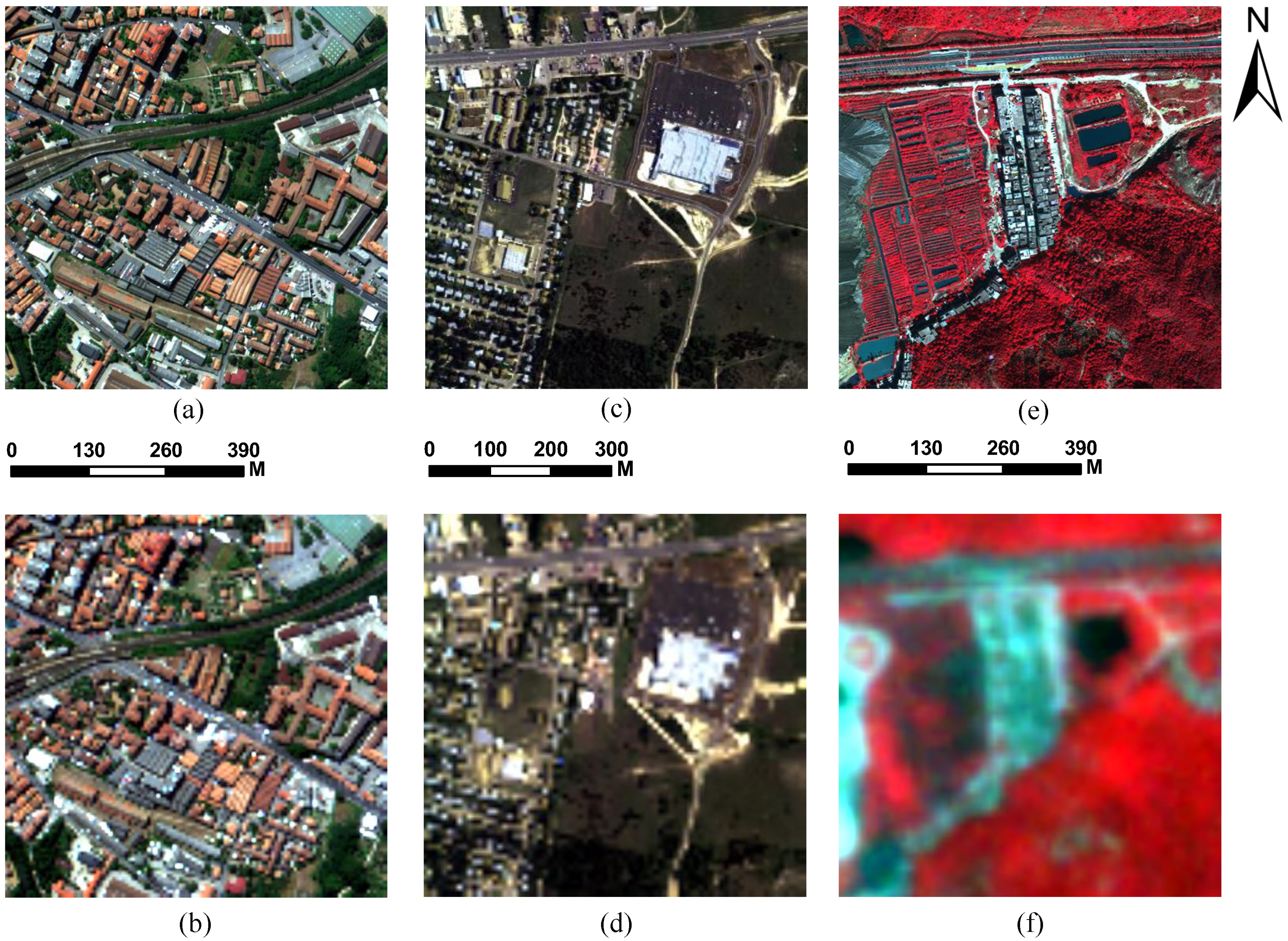
3.2. Experiment Data Sets
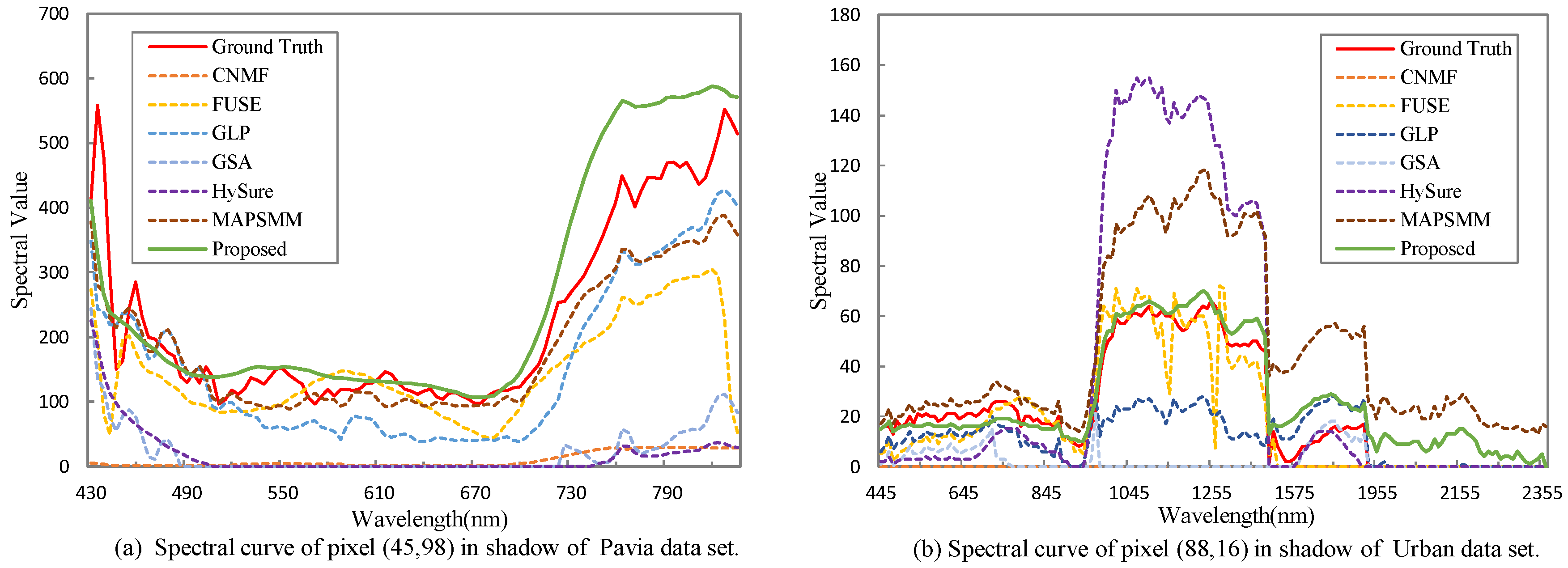
We considered two sets of simulation data and one set of real data for experiments to evaluate the performance of the proposed method. Simulation datasets are: 1. ROSIS Pavia center, 2. HYDICE Urban; Real dataset: 3. LSR-HS data is from Orbita Hyper Spectral (OHS) and HSR-MS data is from worldview-3 (shown in Figure 3).
  • ROSIS Pavia center dataset
    The city center scene in Pavia is in the northern Italy, and the image was obtained by the Reflective Optics System Imaging Spectrometer (ROSIS-3) sensor with high spatial resolution (1.3 m) and the spectrum range is 430–834 nm (http://www.ehu.eus/ccwintco/index.php). There are 102 effective bands with a size of 1096 × 715 pixels in the image, and in this experiment we use the 480 × 480 pixels in the bottom right part the original image as the experiment data. The number of endmembers in this dataset is six.
  • HYDICE Urban dataset
    The Urban dataset was obtained by the Hyperspectral Digital Imagery Collection Experiment (HYDICE) over the urban in Copperas Cove (http://www.erdc.usace.army.mil/Media/FactSheets/FactSheetArticleView/tabid/9254/Article/610433/hypercube.aspx). The image includes 210 bands with high spatial resuolution (2 m) and the spectrum range is 400 to 2400 nm. After the removal of low-SNR and water absorption bands (1–4, 76, 87, 101–111, 136–153 and 198–210), 162 bands remain. The image size is 307 × 307 pixels, and in order to get a integer scale, we subset the in image as 304 × 304 pixels. The number of endmembers in this dataset is six.
    We use the original datasets as reference images Z . To obtain the LSR-HS images X h , the reference images are first blurred by 9 × 9 Gaussian kernel in the spatial domain and then downsampled by a ratio of 4. As to obtain HSR-MS X m , we directly select the bands whose center wavelengths are the same as landsat 8 from the original reference images. We choose the blue, green, red and NIR channel to simulate the HSR-MS images. For Pavia center dataset, we choose 478 nm, 558 nm, 658 nm and 830 nm, for Urban dataset, we choose 481 nm, 555 nm, 650 nm and 859 nm. Because an HS image with lower spatial resolution contains more noise than an HSR-MS image, we add Gaussian white noises with standard deviation 0.1 and 0.04, respectively [35].
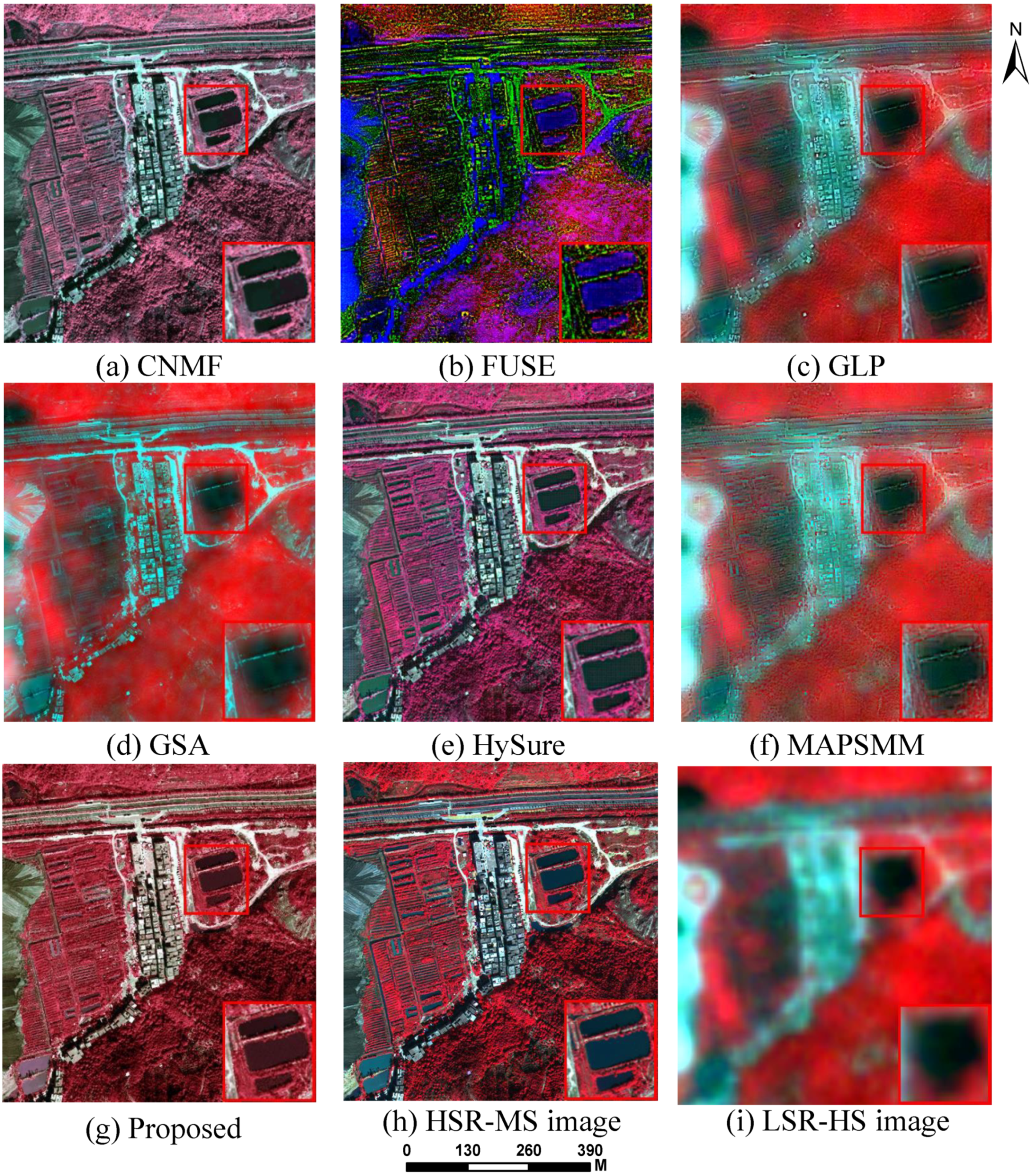
  • Worldview-3 and OHS Hengqin dataset
    The third dataset is Hengqin island area of Guangdong Province, China. The HSR-MS image was captured by worldview-3 on 15 January 2018. The data includes four bands: blue, green, red and NIR, with a spatial resolution of 1.332 m. The LSR-MS image was captured by OHS sensor, which commercial satellites launched by Zhuhai Orbita Aerospace Science and Technology Company in 28 April 2018 carry. The LSR-HS image has 32 bands with 2.5 nm spectral resolution, the spectrum range is 400–1000 nm, and the spatial resolution is 10 m. We discard the 32-th band for the noise, so there are 31 bands left. In this experiment, we choose the area with small change of surface features, which includes water body, vegetation, residential area, highway, etc. The size of HSR-MS image and LSR-HS image in the same experimental area is 500 × 500 and 69 × 69 , respectively. For the convenience of comparative experiment, LSR-HS image was resampled to 100 × 100 (shown in Figure 3). In this experiment, t h r e s h 1 is set as 1.3, and the number of endmembers in this dataset is six.
HS–MS fusion technology obtains HSR-HS images by fusing LSR-HS images and HSR-MS images. Experimental dataset 1 (spatial resolution is 1.3 m) and dataset 2 (spatial resolution is 2 m) are the airborne hyperspectral data, the initial image is HSR-HS data. But for dataset 3, the LSR-HS image is from OHS sensor (10 m), and the HSR-MS image is from worldview3 (1.332 m). We do not have the corresponding area HSR-HS image. So, a ground truth image does not exist for this dataset. In this case, we use mean gradient (MG) [36] to evaluate the fusion results. MG is defined as follows:
M G = g r d x Z ^ + g r d y Z ^
where · is the absolute value. g r d x Z ^ and g r d y Z ^ are the gradients of image Z ^ on the x- and y-axes, respectively. MG can describe the change of texture gray level on the image. It reflects the rate of change in the contrast of small details of the image. In general, the larger the MG is, the more detailed the image information is. The fused HSR-HS image has high spatial resolution, we use MG to evaluate the fusion results. Since MG is originally used to evaluate the accuracy of RGB image not HS image, so we select three bands from fused result to form RGB image (B:3; G:7; R:13), and then evaluate the accuracy. The comparison results of real images showed the applicability of the proposed method.

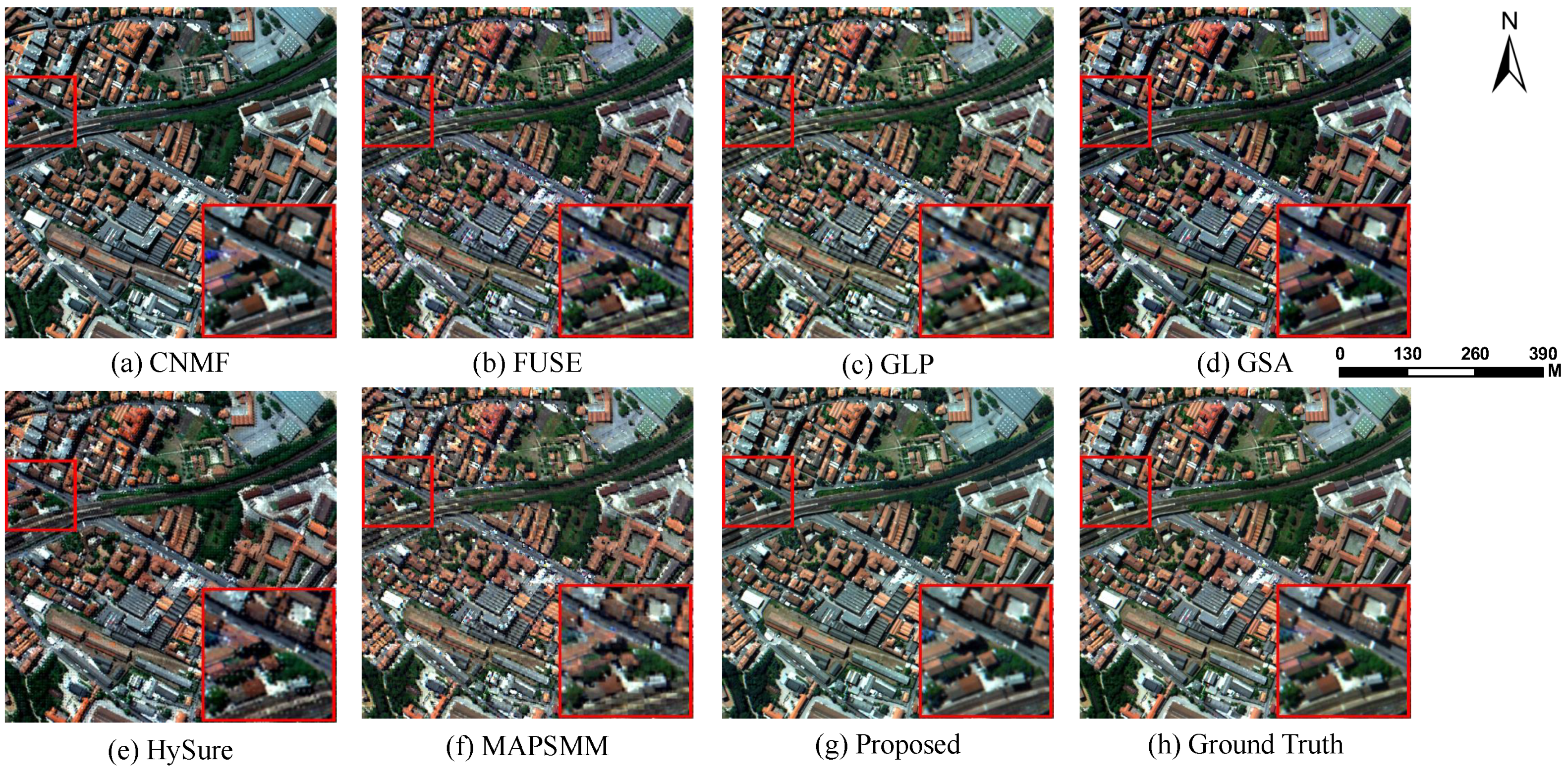
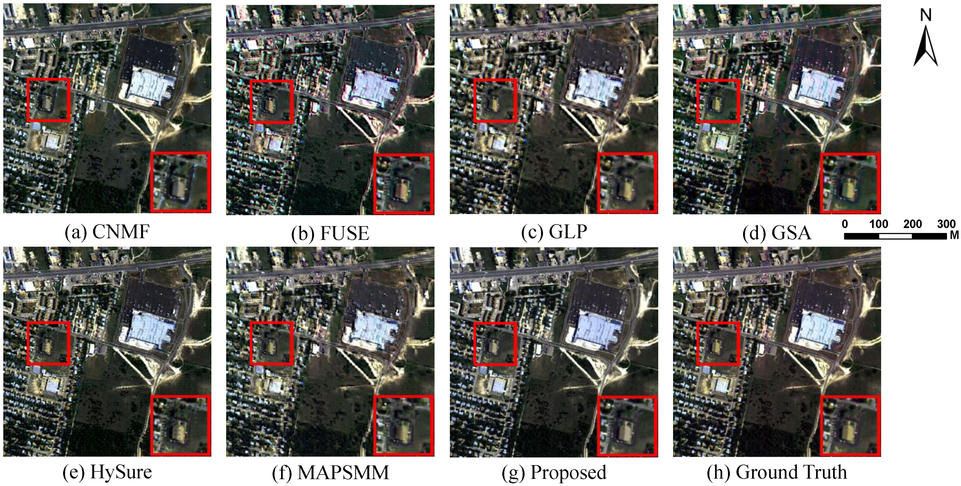
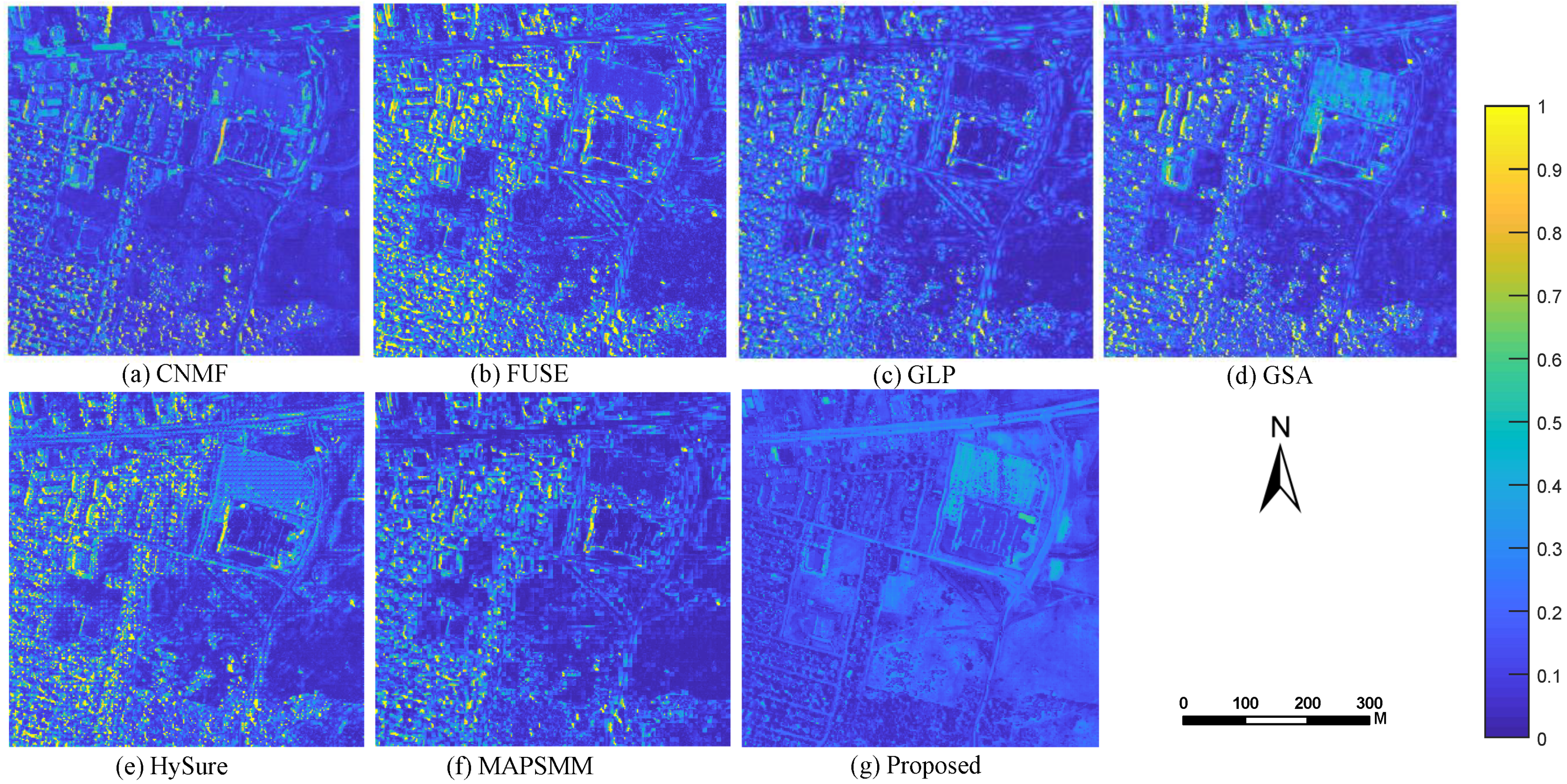
3.3. Experimental Results

To quantitatively evaluate the performance of our method, we compare it with the following methods:
  • CNMF [23] is a well-known HS–MS fusion method based on the spectral unmixing theory.
  • FUSE [18] is one of the Bayesian-based HS–MS fusion algorithms with lower computational cost.
  • GLP [17] determines the difference between the high-resolution image and its low-pass version, and multiplies the gain factor to obtain the spatial details of each low-resolution band.
  • GSA [16] is an adaptive Gram–Schmidt algorithm, which better preserves the spectral information.
  • HySure [20] preserves the edges of the fused image and uses total variation regularization to smooth out noise in homogeneous regions.
  • MAPSMM [21] is the classic baysein-based HS–MS fusion method.

3.3.1. Simulated Dataset Fusion Results

We use PSNR, SAM, ERGAS and Q2n to quantitative evaluate the performances of compared methods, and the results are displayed in Table 1. Figure 4 and Figure 5 show the performance of Pavia Center by fusion results, SAM map, respectively. Figure 6 and Figure 7 show the performance of Urban dataset by fusion results, SAM map, respectively. Figure 8 shows the examples of reconstructed pixel values obtained by the seven methods and the corresponding ground truth.

3.3.2. Real Dataset Fusion Results

Table 2 shows the performance of seven compared methods on the real hengqin dataset. MG and SAM evaluates the sharpness and the spectral distortion of the fusion results, respectively. Figure 9 shows the worldview-3 and OHS data fusion results.

4. Discussion

4.1. Results Discussion

From Table 1, we can see that for two dataset, the proposed method achieves largest PSNR and smallest SAM (except Urban dataset), this means the fused results have the best spatial quality and spectral shape preservation capability, respectively. Moreover, the proposed method also gets the smallest ERGAS value and largest Q2n, this means the result has the overall best quality. For Urban dataset, the SAM of our method result is 8.827, and the smallest SAM 8.665 is from CNMF, it is only a little larger than the best result of the SAM. In addition, the results of the proposed method and CNMF are better than others, this indicates the spectral unmixing-based methods are very promising.
From Figure 4, Figure 5, Figure 6 and Figure 7 the fusion results and SAM map both indicate our method outperforms than other methods. From the fusion results in Figure 4 and Figure 6, we can see there are some spots and mottled textures in the fused images, except our method. Especially from the enlarged part of the fused image (a)–(f), there is some error texture and spectral distortion.
Figure 5 and Figure 7 is the SAM map of Pavia and Urban dataset, respectively. SAM map shows the spectral distortion distribution and degree of the fusion results. We can see from (a)–(f) that the spectral error is mainly distributed in the shadow casted by trees and buildings, which shows that the proposed method can better preserve the spectrum of the shadow part of the LSR-HS images among the comparative methods. In Figure 8, (a) is a pixel value curve in shadow (45, 98), the fusion result of the proposed method better preserves the spectral details of the ground objects in the image. (b) shows the curves are the spectral value of a pixel (88, 16), which is the vegetation in shadow. The result curve of proposed method is the closest one to the ground truth among other compared methods. In addition, fusion results of CNMF are also good, which indicates the methods based on spectral unmixing are very promising.
For the real dataset from worldview3 and OHS Hengqin area, we can see from Table 2 that the proposed method has the largest MG. As we introduced before, the larger the MG value, the finer the fused image quality in detail. Because the HSR-HSI image does not exist in the real case, we use the LSR-HSI image as the reference image for evaluating the spectral accurate of the fusion image. Our method ensures the spectral reliability and improves the spatial resolution of the image. Figure 9 shows the HS–MS fusion results among seven compared methods on the Henqin dataset. From the results, fused images in (a)–(f) cannot achieve good results and produce the spectral distortion. Although (a) and (e) reconstructed the spatial detail, the water body (enlarged part) still have some unsmooth textures and the whole image have spectral distortions. From (c) and (f), the results keep the spectral information of the LSR-HS image, but the reconstructed edges are blurred. The proposed method outperforms the other approaches in that it keeps the spatial and spectral information to a large extent.

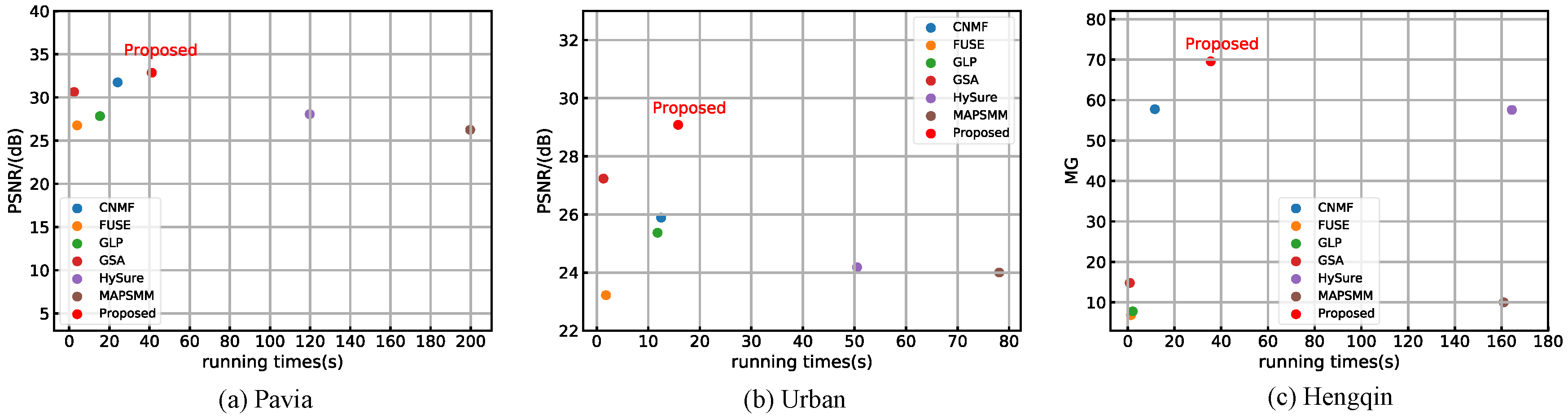
4.2. Time Complexity

Figure 10 shows the running time of all algorithms. The running time of HySure and MAPSMM algorithms are much longer than the rest of MS–HS fusion methods. Although CNMF has a better running time performance of Pavia dataset, its PSNR is lower than that of our method. For Urban dataset, GSA has the smallest time consumption but the PSNR is still smaller than the proposed method. In the Hengqin dataset, our method has the highest MG with moderate running time. In conclusion, our method is slightly slower than some methods but with the best performance. We implemented all algorithms in the experiments under the same hardware configuration: Intel Core i7-8565 U CPU @ 2.00 GHz.

5. Conclusions

This paper proposes a new fusion method based on spectral unmixing by reconstructing HSR-HS images from LSR-MS images and HSR-HS images with a temporal difference. The method is very simple with small computation cost. Considering the temporal difference of two input images, we mask the ground feature changed areas, and then obtain consistent endmembers and corresponding pixels’ positions from the remaining area in LSR-HS images. According to the LSR-HS image endmember spatial information, we can obtain the abundance matrix of an HSR-MS image. Finally, the HS–MS image is generated by the endmember matrix from the LSR-HS image and abundance matrix from the HSR-MS image. The most important thing is this method works well with the images which have a time difference. Furthermore, experimental results of our method in both simulated and real datasets achieve good visual effect, with the best accuracy among the compared methods.
In future work, we plan to apply the endmember spatial information idea to other real datasets from different sensors to improve the universality of this method. From the real image fusion experiment, our method still needs to improve the ability to reduce the spectral distortion while enhancing the spatial resolution of reconstructed images. Therefore, we also plan to further study the correlation between the spatial structure and spectral characteristics of the details by considering the segmentation of the images.

Author Contributions

X.F. and L.H. conceived and designed the experiments; X.F. performed the experiments, analyzed the data, and wrote the paper; L.H. reviewed the paper and helped with the experiments. Q.C. administrated project and supported with the resources. X.L. and Y.Y. helped with the resources. All authors have read and agreed to the published version of the manuscript.

Funding

This work was supported in part by the National key R&D plan on strategic international scientific and technological innovation cooperation special project under Grant 2016YFE0202300, the National Natural Science Foundation of China under Grants 41771452, 41771454 and 41890820, the Natural Science Fund of Hubei Province in China under Grant 2018CFA007.

Acknowledgments

The authors would like to thank the anonymous reviewers for their hard work and the “Innovation and entrepreneurship training program for university Students (S2019619003)” project.

Conflicts of Interest

The authors declare no conflict of interest.

References

  1. Bioucas-Dias, J.M.; Plaza, A.; Camps-Valls, G.; Scheunders, P.; Nasrabadi, N.; Chanussot, J. Hyperspectral remote sensing data analysis and future challenges. IEEE Geosci. Remote Sens. Mag. 2013, 1, 6–36. [Google Scholar] [CrossRef] [Green Version]
  2. Shao, Z.; Fu, H.; Li, D.; Altan, O.; Cheng, T. Remote sensing monitoring of multi-scale watersheds impermeability for urban hydrological evaluation. Remote Sens. Environ. 2019, 232, 111338. [Google Scholar] [CrossRef]
  3. Shao, Z.; Zhang, L.; Zhou, X.; Ding, L. A novel hierarchical semisupervised SVM for classification of hyperspectral images. IEEE Geosci. Remote Sens. Lett. 2014, 11, 1609–1613. [Google Scholar] [CrossRef]
  4. Shao, Z.; Zhou, W.; Cheng, Q.; Diao, C.; Lei, Z. An effective hyperspectral image retrieval method using integrated spectral and textural features. Sens. Rev. 2015, 35, 274–281. [Google Scholar] [CrossRef]
  5. Li, W.; Wu, G.; Zhang, F.; Du, Q. Hyperspectral image classification using deep pixel-pair features. IEEE Trans. Geosci. Remote Sens. 2016, 55, 844–853. [Google Scholar] [CrossRef]
  6. Ma, Y.; Zhang, Y.; Mei, X.; Dai, X.; Ma, J. Multifeature-Based Discriminative Label Consistent K-SVD for Hyperspectral Image Classification. IEEE J. Sel. Top. Appl. Earth Obs. Remote Sens. 2019, 12, 4995–5008. [Google Scholar] [CrossRef]
  7. Shao, Z.; Zhang, L. Sparse dimensionality reduction of hyperspectral image based on semi-supervised local Fisher discriminant analysis. Int. J. Appl. Earth Obs. Geoinf. 2014, 31, 122–129. [Google Scholar] [CrossRef]
  8. Zhang, L.; Weng, Q.; Shao, Z. An evaluation of monthly impervious surface dynamics by fusing Landsat and MODIS time series in the Pearl River Delta, China, from 2000 to 2015. Remote Sens. Environ. 2017, 201, 99–114. [Google Scholar] [CrossRef]
  9. Jiang, J.; Ma, J.; Chen, C.; Wang, Z.; Cai, Z.; Wang, L. SuperPCA: A superpixelwise PCA approach for unsupervised feature extraction of hyperspectral imagery. IEEE Trans. Geosci. Remote Sens. 2018, 56, 4581–4593. [Google Scholar] [CrossRef] [Green Version]
  10. Shao, Z.; Cai, J.; Fu, P.; Hu, L.; Liu, T. Deep learning-based fusion of Landsat-8 and Sentinel-2 images for a harmonized surface reflectance product. Remote Sens. Environ. 2019, 235, 111425. [Google Scholar] [CrossRef]
  11. Yokoya, N.; Grohnfeldt, C.; Chanussot, J. Hyperspectral and multispectral data fusion: A comparative review of the recent literature. IEEE Geosci. Remote Sens. Mag. 2017, 5, 29–56. [Google Scholar] [CrossRef]
  12. He, L.; Wang, M.; Zhu, Y.; Chang, X.; Feng, X. Image Fusion for High-Resolution Optical Satellites Based on Panchromatic Spectral Decomposition. Sensors 2019, 19, 2619. [Google Scholar] [CrossRef] [PubMed] [Green Version]
  13. Loncan, L.; De Almeida, L.B.; Bioucas-Dias, J.M.; Briottet, X.; Chanussot, J.; Dobigeon, N.; Fabre, S.; Liao, W.; Licciardi, G.A.; Simoes, M.; et al. Hyperspectral pansharpening: A review. IEEE Geosci. Remote Sens. Mag. 2015, 3, 27–46. [Google Scholar] [CrossRef] [Green Version]
  14. Carper, W.; Lillesand, T.; Kiefer, R. The use of intensity-hue-saturation transformations for merging SPOT panchromatic and multispectral image data. Photogramm. Eng. Remote Sens. 1990, 56, 459–467. [Google Scholar]
  15. Laben, C.A.; Brower, B.V. Process for Enhancing the Spatial Resolution of Multispectral Imagery Using Pan-Sharpening. U.S. Patent 6,011,875, 4 January 2000. [Google Scholar]
  16. Aiazzi, B.; Baronti, S.; Selva, M. Improving component substitution pansharpening through multivariate regression of MS + Pan data. IEEE Trans. Geosci. Remote Sens. 2007, 45, 3230–3239. [Google Scholar] [CrossRef]
  17. Aiazzi, B.; Alparone, L.; Baronti, S.; Garzelli, A.; Selva, M. MTF-tailored multiscale fusion of high-resolution MS and Pan imagery. Photogramm. Eng. Remote Sens. 2006, 72, 591–596. [Google Scholar] [CrossRef]
  18. Wei, Q.; Dobigeon, N.; Tourneret, J.Y. Fast fusion of multi-band images based on solving a Sylvester equation. IEEE Trans. Image Process. 2015, 24, 4109–4121. [Google Scholar] [CrossRef] [Green Version]
  19. Zhang, Y.; De Backer, S.; Scheunders, P. Noise-resistant wavelet-based Bayesian fusion of multispectral and hyperspectral images. IEEE Trans. Geosci. Remote Sens. 2009, 47, 3834–3843. [Google Scholar] [CrossRef]
  20. Simões, M.; Bioucas-Dias, J.; Almeida, L.B.; Chanussot, J. A convex formulation for hyperspectral image superresolution via subspace-based regularization. IEEE Trans. Geosci. Remote Sens. 2014, 53, 3373–3388. [Google Scholar] [CrossRef] [Green Version]
  21. Eismann, M.T.; Hardie, R.C. Application of the stochastic mixing model to hyperspectral resolution enhancement. IEEE Trans. Geosci. Remote Sens. 2004, 42, 1924–1933. [Google Scholar] [CrossRef]
  22. Keshava, N.; Mustard, J.F. Spectral unmixing. IEEE Signal Process. Mag. 2002, 19, 44–57. [Google Scholar] [CrossRef]
  23. Yokoya, N.; Yairi, T.; Iwasaki, A. Coupled nonnegative matrix factorization unmixing for hyperspectral and multispectral data fusion. IEEE Trans. Geosci. Remote Sens. 2011, 50, 528–537. [Google Scholar] [CrossRef]
  24. Akhtar, N.; Shafait, F.; Mian, A. Sparse spatio-spectral representation for hyperspectral image super-resolution. In European Conference on Computer Vision; Springer: Cham, Switzerland, 2014; pp. 63–78. [Google Scholar]
  25. Lanaras, C.; Baltsavias, E.; Schindler, K. Hyperspectral super-resolution by coupled spectral unmixing. In IEEE International Conference on Computer Vision; Springer: Cham, Switzerland, 2015; pp. 3586–3594. [Google Scholar]
  26. Wang, X.; Zhong, Y.; Zhang, L.; Xu, Y. Spatial group sparsity regularized nonnegative matrix factorization for hyperspectral unmixing. IEEE Trans. Geosci. Remote Sens. 2017, 55, 6287–6304. [Google Scholar] [CrossRef]
  27. Huang, B.; Song, H.; Cui, H.; Peng, J.; Xu, Z. Spatial and spectral image fusion using sparse matrix factorization. IEEE Trans. Geosci. Remote Sens. 2013, 52, 1693–1704. [Google Scholar] [CrossRef]
  28. Nascimento, J.M.; Dias, J.M. Vertex component analysis: A fast algorithm to unmix hyperspectral data. IEEE Trans. Geosci. Remote Sens. 2005, 43, 898–910. [Google Scholar] [CrossRef] [Green Version]
  29. Lawson, C.L.; Hanson, R.J. Solving Least Squares Problems; Siam: Ann Arbor, MI, USA, 1995; Volume 15. [Google Scholar]
  30. Bioucas-Dias, J.M.; Plaza, A.; Dobigeon, N.; Parente, M.; Du, Q.; Gader, P.; Chanussot, J. Hyperspectral unmixing overview: Geometrical, statistical, and sparse regression-based approaches. IEEE J. Sel. Top. Appl. Earth Obs. Remote Sens. 2012, 5, 354–379. [Google Scholar] [CrossRef] [Green Version]
  31. Wycoff, E.; Chan, T.H.; Jia, K.; Ma, W.K.; Ma, Y. A non-negative sparse promoting algorithm for high resolution hyperspectral imaging. In Proceedings of the IEEE International Conference on Acoustics, Speech and Signal Processing, Vancouver, BC, Canada, 26–31 May 2013; pp. 1409–1413. [Google Scholar]
  32. Kruse, F.A.; Lefkoff, A.; Boardman, J.; Heidebrecht, K.; Shapiro, A.; Barloon, P.; Goetz, A. The spectral image processing system (SIPS)—interactive visualization and analysis of imaging spectrometer data. Remote Sens. Environ. 1993, 44, 145–163. [Google Scholar] [CrossRef]
  33. Wald, L. Quality of high resolution synthesised images: Is there a simple criterion? In Proceedings of the Third Conference “Fusion of Earth Data: Merging point Measurements, Raster Maps and Remotely Sensed Images”, Sophia Antipolis, France, 26–28 January 2000; pp. 99–103. [Google Scholar]
  34. Wang, Z.; Bovik, A.C. A universal image quality index. IEEE Signal Process. Lett. 2002, 9, 81–84. [Google Scholar] [CrossRef]
  35. Takeyama, S.; Ono, S.; Kumazawa, I. Hyperspectral and Multispectral Data Fusion by a Regularization Considering. In Proceedings of the ICASSP 2019-2019 IEEE International Conference on Acoustics, Speech and Signal Processing (ICASSP), Brighton, UK, 12–17 May 2019; pp. 2152–2156. [Google Scholar]
  36. Lu, T.; Wang, J.; Zhang, Y.; Wang, Z.; Jiang, J. Satellite Image Super-Resolution via Multi-Scale Residual Deep Neural Network. Remote Sens. 2019, 11, 1588. [Google Scholar] [CrossRef] [Green Version]
Figure 1. Overall flowchart of the proposed hyperspectral–multispectral (HS–MS) fusion method (Image in the flowchart has six endmembers).
Remotesensing 12 01009 g001
Figure 2. Pure pixel in low spatial resolution (LSR)-HS image and high spatial resolution (HSR)-MS image.
Remotesensing 12 01009 g002
Figure 3. Experiment datasets. ((a)Pavia HSR-MS image (B:13, G:33, R:58); (b) Pavia LSR-HS image (downsampled ratio:4, add noise); (c) Urban HSR-MS image (B:17, G:37, R:50); (d) Urban LSR-HS image (downsampled ratio:4, add scale); (e) Hengqin HSR-MS image (B:2, G:3, R:4); (f) Hengqin LSR-HS image (B:8, G:13, R:27). Scale 4 is the downsampled ratio.)
Remotesensing 12 01009 g003
Figure 4. HS–MS fusion results among seven compared methods and ground truth on ROSIS Pavia Center dataset with one demarcated areas zoomed in 1.5 times for easy observation. The composite HSIs are shown with bands 58-33-13 as R-G-B. (a) Coupled nonnegative matrix factorization (CNMF). (b) Fast fusion based on Sylvester equation (FUSE). (c) Generalized Laplacian pyramid (GLP). (d) Gram–Schmidt (GS). (e) HS Superresolution (HySure). (f) MAPSMM. (g) Proposed method. (h) Ground truth.
Remotesensing 12 01009 g004
Figure 5. HS–MS fusion Spectral Angle Mapper (SAM) map results among seven compared methods on ROSIS Pavia Center dataset. (a) CNMF. (b) FUSE. (c) GLP. (d) GS. (e) HySure. (f) MAPSMM. (g) Proposed method. The color scale denotes the spectral angle difference of each pixel between the ground truth to the fused image (from 0 to 1).
Remotesensing 12 01009 g005
Figure 6. HS–MS fusion results among seven compared methods and ground truth on HYDICE Urban dataset with one demarcated areas zoomed in 1.5 times for easy observation. The composite HSIs are shown with bands 50-37-17 as R-G-B. (a) CNMF. (b) FUSE. (c) GLP. (d) GS. (e) HySure. (f) MAPSMM. (g) Proposed method. (h) Ground truth.
Remotesensing 12 01009 g006
Figure 7. HS–MS fusion SAM map results among seven compared methods on HYDICE Urban dataset. (a) CNMF. (b) FUSE. (c) GLP. (d) GS. (e) HySure. (f) MAPSMM. (g) Proposed method. The color scale denotes the spectral angle difference of each pixel between the ground truth to the fused image (from 0 to 1).
Remotesensing 12 01009 g007
Figure 8. Spectral value curves of the pixel in (45, 98) pixel of Pavia dataset and (88, 16) pixel of Urban dataset, respectively, using the seven compared methods compared to the ground truth.
Remotesensing 12 01009 g008
Figure 9. HS–MS fusion results among seven compared methods on Hengqin dataset with one demarcated areas zoomed in 1.5 times for easy observation. The composite HSIs are shown with bands 27-13-8 as R-G-B. (a) CNMF. (b) FUSE. (c) GLP. (d) GS. (e) HySure. (f) MAPSMM. (g) Proposed method. (h) HSR-MS image. (i) LSR-HS image.
Remotesensing 12 01009 g009
Figure 10. Running time (seconds) of three datasets for different MS–HS fusion algorithms.
Remotesensing 12 01009 g010
Table 1. Experimental evaluation metrics among seven compared methods on two simulated Dataset (Bold numbers indicate the best performance).
DataIndexMethod
CNMFFUSEGLPGSAHySureMAPSMMProposed
PaviaPSNR31.74726.76627.83830.63628.06126.25532.860
SAM6.35713.6468.64311.77411.8769.6295.700
ERGAS4.9738.6677.4485.4607.3348.9224.799
Q2n0.9290.8360.8520.9350.8880.7920.942
UrbanPSNR25.89023.22325.37027.23524.18324.00229.083
SAM8.66515.1908.68911.30713.9469.5468.827
ERGAS7.36110.2407.7156.1809.0089.0285.745
Q2n0.8630.7720.8170.8860.8020.7720.933
Table 2. MG and SAM of HS–MS fusion results among seven compared methods on Hengqin dataset (Bold numbers indicate the best performance).
MethodHengqin
CNMFFUSEGLPGSAHySureMAPSMMProposed
MG57.7436.8527.79114.81257.5709.99669.575
SAM4.40780.2761.5464.5898.2392.4354.849

