Article

Glacier Mass Balance in the Nyainqentanglha Mountains between 2000 and 2017 Retrieved from ZiYuan-3 Stereo Images and the SRTM DEM

1
State Key Laboratory of Remote Sensing Science, Aerospace Information Research Institute, Chinese Academy of Sciences, Beijing 100101, China
2
University of Chinese Academy of Sciences, Beijing 100049, China
3
Faculty of Civil Engineering and Earth Sciences, Delft University of Technology, 2628 Delft, The Netherlands
4
Institute of Tibetan Plateau Research, Chinese Academy of Sciences, Beijing 100101, China
*
Author to whom correspondence should be addressed.
Remote Sens. 2020, 12(5), 864; https://doi.org/10.3390/rs12050864
Submission received: 17 January 2020 / Revised: 19 February 2020 / Accepted: 3 March 2020 / Published: 7 March 2020
(This article belongs to the Special Issue Cryospheric Remote Sensing III)

Abstract

:
Mountain glaciers are excellent indicators of climate change and have an important role in the terrestrial water cycle and food security in many parts of the world. Glaciers are the major water source of rivers and lakes in the Nyainqentanglha Mountains (NM) region, where the glacier area has the second largest extent on the Tibetan Plateau. The potential of the high spatial resolution ZiYuan-3 (ZY-3) Three-Line-Array (TLA) stereo images to retrieve glacier mass balance has not been sufficiently explored. In this study, we optimized the procedure to extract a Digital Elevation Model (DEM) from ZY-3 TLA stereo images and estimated the geodetic mass balance of representative glaciers in the two typical areas of the NM using ZY-3 DEMs and the C-band Shuttle Radar Topography Mission (SRTM) DEM in three periods, i.e., 2000–2013, 2013–2017 and 2000–2017. The results provide detailed information towards better understanding of glacier change and specifically show that: (1) with our new stereo procedure, ZY-3 TLA data can significantly increase point cloud density and decrease invalid data on the glacier surface map to generate a high resolution (5 m) glacier mass balance map; (2) the glacier mass balance in both the Western Nyainqentanglha Mountains (WNM) and Eastern Nyainqentanglha Mountains (ENM) was negative in 2000–2017, and experienced faster mass loss in recent years (2013–2017) in the WNM. Overall, the glaciers in the western and eastern NM show different change patterns since they are influenced by different climate regimes; the glacier mass balances in WNM was –0.22 ± 0.23 m w.e. a−1 and –0.43 ± 0.06 m w.e. a−1 in 2000–2013 and 2013–2017, respectively, while in 2000–2017, it was –0.30 ± 0.19 m w.e. a−1 in the WNM and –0.56 ± 0.20 m w.e. a−1 in the ENM; (3) in the WNM, the glaciers experienced mass loss in 2000–2013 and 2013–2017 in the ablation zone, while in the accumulation zone mass increased in 2000–2013 and a large mass loss occurred in 2013–2017; as regards the ENM, the glacier mass balance was negative in 2000–2017 in both zones; (4) glacier mass balance can be affected by the fractional abundance of debris and glacier slope; (5) the glacier mass balances retrieved by ZY-3 and TanDEM-X data agreed well in the ablation zone, while a large difference occurred in the accumulation zone because of the snow/firn penetration of the X-band SAR signal.

Graphical Abstract

1. Introduction

As one of the major fresh water resources in cold and high elevation regions, mountain glaciers can not only determine the terrestrial water cycle and ecosystem stability in these regions, but also threaten live and food security of the local people [1,2,3]. With global warming, glacier continuous ablation can increase the frequency of many glacial hazards, such as floods and mudslides, and contribute to sea level rise [2,4]. Precise monitoring of mountain glacier elevation change and mass balance is needed to mitigate risks related to these hazards. The High Mountain Asia (HMA), i.e., Tibetan Plateau and its surrounding mountain ranges such as Himalaya, Karakoram, Pamir, and Tien Shan, includes the largest glacial area (~105 km2) outside the Arctic and Antarctica [5]. The mass loss of glaciers in the HMA has been persistent in the recent decades and may still continue in the next decades, which will threaten the existence of more than 0.9 billion people [4,5,6].
Two main remote sensing techniques, i.e., Interferometric Synthetic Aperture Radar (InSAR) and Photogrammetry (Airborne and Spaceborne) have been applied to estimate the glacier elevation change by several authors [7,8,9]. With the successful launch of TerraSAR-X and TanDEM-X (TerraSAR-X/TanDEM-X), the InSAR technique has become one of the promising ways to retrieve glacier thickness change by using data acquired in the two-pass bistatic interferometric mode [9]. Higher accuracy in the retrieved glacier surface elevation is achieved by the SAR signal acquired almost simultaneously by the TerraSAR-X/TanDEM-X satellites, which reduces the phase decoherence in the image pair. The results by the InSAR technique still need to be evaluated by applying independent datasets and methods, however. In addition, this two-pass bistatic interferometric mode is activated only occasionally on-request, which does not provide regular observations and limits the application to monitor glacier mass balance.
Space-borne optical photogrammetry has also been used in several studies to capture the glacier mass balance [9,10,11,12]. Advanced Spaceborne Thermal Emission and Reflection Radiometer (ASTER) stereo images (3N and 3B bands) have been widely used to estimate glacier mass balance [6,13], notwithstanding the sub-optimal matching points on smooth glacier surfaces due to the moderate spatial resolution (i.e., 15 m). Other satellites, such as WorldView and Pléiades, can provide high resolution stereo images by two methods:
(a)
attitude swing or imaging simultaneously the same region from multiple satellites, which is deployed to respond to emergency conditions or special requirements, but cannot provide observations at regular time intervals over a long period of time;
(b)
revisiting the same region at short time intervals, but even though the revisit interval is short, the surface condition may change, as for example due to snowfall events.
The three-line-array (TLA) stereo images, such as the ones acquired by the Advanced Land Observing Satellite (ALOS) and ZiYuan-3 (ZY-3), consist of three high resolution images at Nadir (N), Backward (B) and Forward (F) view angles and can form three pairs of nearly-simultaneous stereo images (NB: Nadir-Backward, NF: Nadir-Forward, BF: Backward-Forward). This kind of image data has been used less frequently to monitor glacier mass balance. To our knowledge, the procedure to analyze TLA stereo images can be further improved to increase the accuracy of estimated glacier elevation and its changes. For example, the horizontal and vertical systematic errors have not been considered before fusing the different point clouds generated by applying different view angles combinations, which may introduce large errors in the final DEMs [14].
One of the key techniques to increase the accuracy of the retrieved elevation is to match more points on the glacier surface. Dense matching algorithms may be a reliable option and have been applied in low brightness contrast and smooth texture regions, such as buildings and forest. The Semi-Global dense Matching (SGM) technique has been applied to glacier change research using Unmanned Aerial Vehicle (UAV) stereo images [15,16,17]. For instance, Dall’Asta et al. [18] and Rieg et al. [14] successfully employed SGM to acquire rock glacier displacement and mass balance by UAV and Pléiades stereo images. The applications of this technique to satellite TLA stereo images to retrieve changes in glacier elevation have been limited, however. The analysis of the TLA stereo images at high spatial resolution yields multiple elevation estimates within each grid of the DEM to be generated. Potential outliers need to be removed prior to the construction of the DEM. Suitable filters have been developed and applied to generate a DEM from a Light Detection and Ranging (LiDAR) point cloud and some can be applied to detect and remove outliers in point clouds generated from satellite stereo images [14,19,20]. A filter used to identify and remove outliers in a LiDAR point cloud was applied in the study by Skinner et al. [21] .
The Nyainqentanglha Mountains (NM) is the second largest glacier region in the Tibetan Plateau. The glacier area in the NM region is about 9600 km2 and there are many rivers and lakes, such as Parlung Zangbo River and Nam Co Lake [22]. Parlung Zangbo River originates from the Ranwu lake in the ENM, which is near the Yalung glacier terminus and receives meltwater from glaciers. One of the important contributions to the water balance of the Nam Co Lake is the runoff from glaciers in the WNM. Previous studies suggest that this runoff also contributes to the increase in water volume stored in the lake [23,24]. Not only these rivers and lakes directly provide fresh water for local people, but also guarantee their food security by contributing to water supply for grassland, livestock and farmland. The topography of the Eastern Nyainqentanglha Mountains (ENM) is more complex than that in the Western Nyainqentanglha Mountains (WNM). The glaciers in these two regions belong to maritime (in ENM) and subcontinental (in WNM) types, respectively; the NM is an ideal site to test the performance of ZY-3 TLA data to retrieve glaciers elevation and their changes in different kinds of terrain.
Glacier mass balance is affected by climate variability and human activity. Firstly, with weakening Indian monsoon, the precipitation decreased and air temperature increased in the Himalaya and southeast Tibet Plateau in the past decades, which increased mass loss of glaciers in both regions [5,13,25]. On the other hand, strengthening westerlies led to an increase in precipitation in some regions of Karakoram, Pamir and Kunlun and mass gains in these regions [5,13,26]. Secondly, the effects of human activity cannot be neglected because pollutants, dust and black carbon may deposit on the glacier and snow surface and decrease their albedo and increase irradiance absorbed by glaciers, leading to larger mass loss [27,28,29,30]. In the NM, previous studies have documented that glacier mass loss is caused by both factors. On the one hand, in the WNM, the decreasing precipitation and increasing air temperature caused by the weakening Indian monsoon led to negative glacier mass balance, while in the ENM, the increasing air temperature did offset the slight increase in precipitation and led to mass loss in the past three decades [9,31]. On the other hand, field measurement and model results in the Zhadang glacier show that black carbon is a main factor of lower glacier albedo, with the contribution of dust and black carbon to the reduction in glacier albedo being up to 84% [32].
Previous studies reported negative glacier mass balances in both regions in the first decade of the 21st century, while the magnitudes of mass loss calculated by different data, e.g., field observation, ICESat/GLAS (Ice, Cloud and land Elevation Satellite/Geoscience Laser Altimeter System) and TerraSAR-X/TanDEM-X, were not consistent [5,9,33,34]. Furthermore, the different time spans of the above-mentioned studies make it difficult to cross-validate spatial patterns of glacier mass balance. Therefore, it is also interesting to compare changes in glacier elevation and mass balance under different dominant climate in these two sub-regions over time using the ZY-3 TLA data, which have never been used in this region before.
The purposes of this study are:
  • To develop an improved procedure to retrieve glacier mass balance from ZY-3 TLA stereo images;
  • To evaluate the performance of ZY-3 stereo images in deriving glacier mass balance over the complex terrain in the ENM and relatively smoother terrain in the WNM;
  • To cross-validate optical photogrammetry (ZY-3 TLA stereo images) and InSAR (TerraSAR-X and TanDEM-X image pairs) in capturing the spatial patterns of glacier mass balance and explore their differences;
  • To compare and analyze the trends in the mass balance of glaciers responding to maritime climate in the ENM and to subcontinental climate in the WNM in the first decade (2000–2013) and in recent years (2013–2017).

2. Study Area and Datasets

2.1. Study Area

Both study sites belong to the NM (Figure 1). One lies in the central WNM, which is a gentle terrain region, where the mean slope in the whole region is 20° and its elevation range is 4150–7100 m a.s.l. (Figure 1a). Weather in summer and winter is dominated by both the Indian monsoon and the Westerlies, respectively. The annual air temperature and precipitation are in the ranges −0.6–2.8 °C and 37–500 mm, respectively [35]. The Nam Co Lake, the second largest lake in the Tibetan Plateau, is located in the north of the NM area along the northern side of the glacier area. The glacier is subcontinental type in the WNM, and only five glaciers were reported to be debris-covered in the ablation zone [36]. The glacier area covered by our data is about 471.3 km2 (i.e., 68.1% of the whole glacial area in the WNM) and the equilibrium-line altitude (ELA) is 5800 m a.s.l. [37]. Glaciers in the WNM shrunk during 1976–2009, with the glacier area shrinking by 9.9% ± 3.1% during the entire period [36].
The second study area is located in the Kangri Karpo mountains in the ENM. The topography is more complex than that in the WNM with the mean slope reaching to 26° and the elevation range being 2000–6550 m a.s.l. (Figure 1b). Compared with the WNM, the climate of this region is more dominated by the Indian monsoon and less affected by Westerlies [5]. As the moistest sector of the Tibetan Plateau, the annual precipitation reaches 2000–3000 mm in this region. The two main rivers, Yarlung Tsangpo River and Gongri–Gabo River, are in the north and south of the study area. The glaciers in this region belong to the maritime type, the ELA is 5400 m a.s.l. and there are many glaciers where the terminal snouts are covered by debris [31]. Our data cover 772.7 km2 glaciers in the two sub-basins in the ENM, i.e., the 5O282B basin and the 5O291B basin as defined by the 2nd Chinese Glacier Inventory (CGI2) [22,38]. The glaciers in Kangri Karpo mountains experienced a large retreat in the past four decades, with the entire glacier area decreased by 24.9% ± 2.2% from 1980 to 2015 [31].

2.2. Datasets

2.2.1. ZY-3

As the first Chinese civilian high-resolution stereo mapping satellite, ZY-3 satellite can provide more than 7 years of regulation observations with launching on 9 January 2012 [39]. It can compose TLA stereo images by three panchromatic sensors at three view angles (nadir, forward and backward). One scene of ZY-3 TLA data includes nadir (N, 0°), backward (B, −23.5°) and forward (F, +23.5°) images at spatial resolutions 2.5 m, 3.5 m and 3.5 m, respectively. The rational polynomial coefficients (RPCs) applying to the WGS84/WGS84 (geocentric coordinate system and elevation reference) are delivered together with the ZY-3 image data, which provide the mathematical transformation from geographical coordinates to image coordinates [40]. Notwithstanding the impact cloud cover, 14 ZY-3 cloudless image data sets are available from 2012 to 2017. In this study, we selected four of them to estimate the glacier mass balance in the study area (Table 1). With the launch of the second satellite of ZY-3 series (ZY-3 02) in 2016, the temporal repeat improves from 5 days with only one satellite to 3 days. Moreover, the third satellite will be launched in 2020, which will further increase available cloudless images.

2.2.2. SRTM

A global DEM dataset at 30 m × 30 m resolution was generated by using the data in C-band and X-band from the Shuttle Radar Topography Mission (SRTM) acquired from 11 to 22 February 2000 by the United States Geological Survey (USGS) and German Aerospace Center (DLR). The C-band SRTM (SRTM-C) DEM was used as reference glacier surface elevation in 2000 and vertical reference for the off-glacier region in ZY-3 DEMs assuming no elevation change in the off-glacier region during our study period. The difference between the X-band SRTM (SRTM-X) and SRTM-C DEMs was applied to estimate C-band SAR signal penetration depth in the glacier region. The elevation reference of SRTM DEMs was transformed from Earth Gravity Model 1996 geoid (EGM96) to 1984 World Geodetic System (WGS84) geoid, and the resolution was resampled to 5 m using bilinear interpolation to generate high resolution ZY-3 DEMs and glacier elevation maps.

2.2.3. Glacier Elevation Change Map from DInSAR

The glacier elevation change maps between 2000 and 2014 in the WNM and ENM obtained by differential synthetic aperture radar interferometry (DInSAR) technique using TerraSAR-X/TanDEM-X images and SRTM DEM were provided by Li et al. [9] and Wu et al. [31]. Here, we used these maps to explore the difference between optical photogrammetry and DInSAR in retrieving the spatial pattern of glacier mass balance and to estimate the penetration depth of X-band SAR signal. More details on the glacier elevation change retrieved from DInSAR data can be found in Li et al. [9] and Wu et al. [31].

2.2.4. Landsat TM data

In this study, two Landsat Thematic Mapper (TM) images on 8 September 2005 and 2 November 2009 were used to classify debris-covered and clean-ice regions in the ENM and WNM, respectively (Table 1).

3. Methodology

The geodetic method with DEM differencing technique was applied to estimate the glacier mass balance using the ZY-3 TLA stereo images. The proposed approach consists of two main procedures: (1) applying an improved method to generate ZY-3 DEM raster data at high spatial resolution (Section 3.1); (2) glacier mass balance estimation using the generated ZY-3 DEMs data (Section 3.2). The methodology details will be described in the sections below and Figure 2 gives the general workflow.

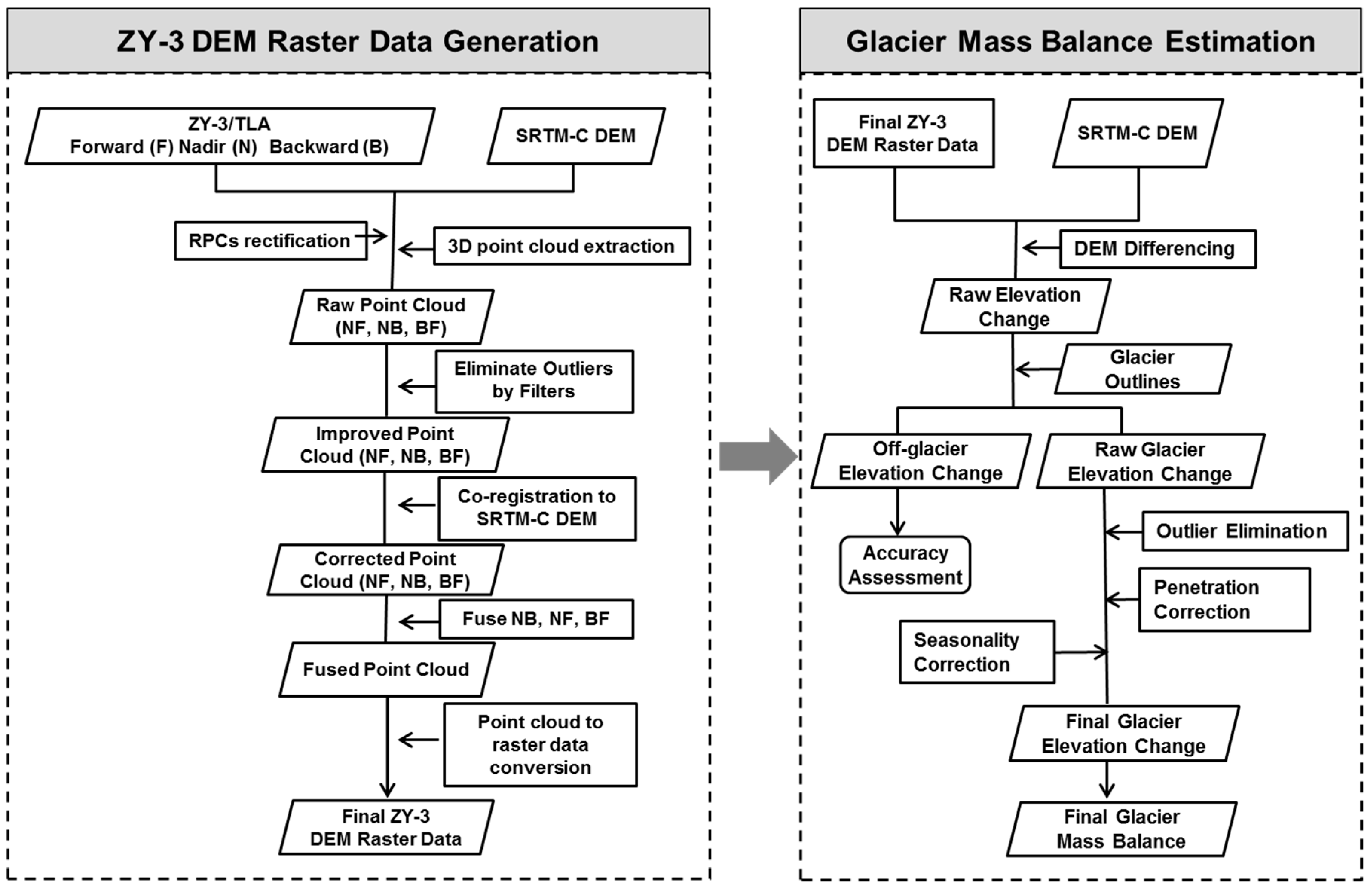
3.1. ZY-3 DEM Raster Data Generation

This procedure includes three steps. The first step, i.e., stereo image processing of ZY-3 data, is to generate point clouds from different view image combinations; the second step includes registering the ZY-3 point clouds to SRTM and bias correction; the last step is to fuse the co-registered point clouds of three combinations of ZY-3 images and to generate final ZY-3 DEM raster data.

3.1.1. Stereo Image Processing of ZY-3 TLA Data

The stereo image processing of ZY-3 TLA data mainly includes RPCs rectification by Control Points (CPs) and raw three-dimensional (3D) point cloud extraction with rectified RPCs files.
RPCs rectification (Figure 2). According to the previous study, taking the SRTM DEM as the reference DEM, the vertical accuracy of the ZY-3 DEM in the mountain region can be improved significantly than that without CPs [41]. Therefore, in order to get more accurate point clouds, the initial RPCs of ZY-3 stereo images need to be rectified by applying a sufficient number of CPs. In this study, we proposed a two-step triangulation measurement to overcome the difficulty of collecting enough CPs. To gather more reference information for triangulation measurements, we applied two types of CPs. On the one hand, at least 10 Ground Control Points (GCPs) were collected within the area imaged to ensure accuracy in triangulation measurement. All such GCPs should be in the overlap region of different ZY-3 TLA stereo images and can be identified with distinct features, such as the intersections of roads and house corners in villages located within the study area. The horizontal coordinates and the elevation values of GCPs were extracted from the high resolution images in Google Earth and the SRTM-C DEM, respectively. On the other hand, we propose to use Elevation Control Points (ECPs) to improve the elevation information towards better rectification when using the RPCs. Unlike the horizontal coordinates of GCPs from Google Earth, ECPs were obtained with the first triangulation measurements based on only the GCPs. The ECPs generation included three steps: (1) the Tie Points (TPs) were automatically obtained by the Least Squares Matching Technique (LSMT), which searches the same feature in the stereo images and achieves sub-pixel matching accuracy; (2) x, y and z coordinates of these TPs were calculated by the first triangulation measurements; (3) the ECPs were created by transforming the z coordinate of TPs to the elevation of SRTM-C DEM. As a result, 986 and 855 (2159 and 2066) ECPs were created in the ENM (WNM) for the years of 2013 and 2017, respectively (see Table 2). Eventually, the triangulation measurement was applied to the GCPs and ECPs for RPCs rectification. The RMSEs (image coordinates) of triangulation measurement in all combinations of view angles were less than 1 pixel (on average 0.44 pixel), and the RMSEs (geospatial coordinates) in horizontal and vertical directions were less than 2.5 m (the averages were 1.50 m in x, 1.80 m in y and 1.12 m in z, respectively). Overall, the performances of the NB and NF pairs were better than the BF pair since the spatial resolution of the N image (2.5 m) is higher than that of the B and F images (3.5 m). Overall, both the RMSEs of image and geospatial coordinates in the ENM were higher than that in the WNM because of more complicated terrain in the ENM.
Raw 3D point cloud extraction (Figure 2). The purposes of this step are to extract a 3D point cloud using rectified RPCs files as well as to remove outliers in the raw point clouds. The Semi-Global Matching (SGM) technique implemented in the ERDAS IMAGINE 2015 software was used to produce the 3D point cloud [14]. Since it takes the image similarity and the parallax field continuity into account, the SGM has been applied in many studies and proved to be an excellent dense matching algorithm [18,42]. The elevation of some points retrieved by ZY-3 TLA images in low contrast and smooth texture areas, such as snow- and ice-covered regions, was much higher or lower than that in the SRTM-C DEM or neighboring points. This suggested inaccurate retrievals because in general glacier elevation is rather smooth over short distances. Two point cloud filters were applied to remove these outliers. According to previous studies [11,31,43], the 3D points with elevation exceeding by 100 m or more the corresponding SRTM-C DEM elevation, were in the glacier margins and mountain shadows and regarded as outliers and they were eliminated first by applying the filter:
P 1   E SRTM   +   100   or   P 1     E SRTM   100
where P 1 is an outlier removed by the filter (Equation (1)), E SRTM is the SRTM elevation. The topography clearly improved after this first filtering. Then a point cloud filter, which is based on the mean elevation ( M P ) and standard deviation ( σ P ) of the elevation of the points in a moving window was applied to remove the remaining outliers, with this filter being:
P 2     M P   +   n p · σ P   or   P 2     M P   n p · σ P   ( n   = 5 ,   4.5 ,   4 ,   3.5 ,   3 )
where P 2 is a removed point after applying the filter (Equation (2)), n p is the multiplier of σ P applied in every iteration. According to previous studies, the elevations exceeding M P by more than three times the standard deviations ( σ P ) were regarded as potential outliers [7,44,45]. Considering that the outliers can affect the calculations of M P and σ P , we adopted n p decreasing from 5 to 3 with 0.5 interval gradually instead of directly setting n = 3 to remove outliers. The size of the filter moving window was set at 30 m × 30 m, i.e., the same as the SRTM-C DEM resolution.

3.1.2. Co-Registration of Point Clouds

Since the horizontal coordinate offsets (x, y) of a point cloud would have a significant influence on the estimation of glacier surface elevation change, we used a robust analytical 3D method to co-register and correct the raw point clouds before fusion [46] (Figure 3). Firstly, all the ZY-3 point clouds were transformed to 5 m spatial resolution ZY-3 DEMs by averaging the elevations within each 5 m × 5 m cell; secondly the offsets calculated by the robust analytical 3D method with ZY-3 and SRTM-C DEMs were added to the ZY-3 point clouds. According to this 3D method, a cosine relationship between cosine parameters (a, b and c) and terrain parameters ( d h , α and φ ) was built as:
d h t a n ( α ) =   a · cos ( b φ ) + c
c = d h ¯ tan ( α ¯ )
where a and b are the magnitude and direction of the shift vector, c is the mean elevation difference ( dh ¯ ) between the two DEMs (i.e., the ZY-3 DEM and SRTM-C DEM in our case) divided by the tangent of the mean terrain slope ( α ¯ ); dh is the elevation difference between the two DEMs, α and φ are the slope and aspect of the terrain. In brief, the shift and elevation biases can be approximately estimated by the parameter a and c . The specific method includes two steps: first, the 3D point clouds were transformed into raster images with 5 m spatial resolution; second, the low and high tails, i.e., the 5% and 95% quantiles, of the distribution of the elevation difference between ZY-3 DEMs and SRTM DEM were removed, and the interquartile ranges (IQR) were re-calculated using the remaining points. Only the values within a range obtained by multiplying by 1.5 the sum of the 2nd and 3rd IQR were used to correct the systematic offsets. The details of the method can be found in Pieczonka et al. [47]. The mean, median, standard deviation (σ) and normalized median absolute deviation [48] of the elevation differences were calculated to evaluate the results of co-registration (Table 3). Normalized Median Absolute Deviation (NMAD) is a more robust estimate of the standard deviation because it is proportional to the median of the absolute differences between the DEM biases and the median of these DEM biases [48,49].
The results obtained with the triangulation measurement (Table 2) and DEMs co-registration (Figure 3 and Table 3) show that overall the horizontal and vertical accuracies of the NB and NF pairs are better than the BF pair. When considering the registration result of the three view angle combinations in the ENM in 2017, the parameters a and c of the 2017NBENM–SRTM-C and 2017NFENM–SRTM-C are smaller than for the 2017NFENM–SRTM-C (Figure 3). In all the images the mean x and y shifts of both NB and NF pairs of the 2017ENM images are 2.74 m and 5.43 m, 2.12 m and 4.07 m, smaller than that for the BF pair with 3.41 m and 7.11 m; the z shift of the NB pair is the smallest (1.73 m) followed by BF (4.35 m) and NF pairs (5.90 m). Moreover, compared with the uncorrected elevations derived from ZY-3 data, the σ and NMAD of the corrected NF elevation difference decreased by 4.45% (range is 2.19–5.91%) and 4.95% (range is 1.85–6.40%), and the corresponding values for BF decreased by 5.05% (range is 3.69–5.63%) and 6.07% (range is 4.07–7.80%) (Table 3). No evident improvements of the σ and NMAD were obtained for the NB pair (Table 3), thus, only the vertical bias correction was applied to the NB elevations.

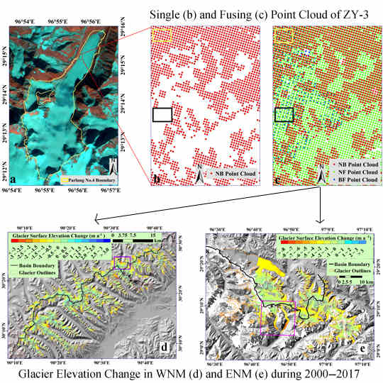
3.1.3. Fusion of Multiple Point Clouds

After co-registration and bias correction, the 3D point clouds data generated by different stereo pairs from the same multi-angular acquisition by ZY-3 TLA were fused to generate the final point clouds (see procedure in Figure 2). The fusion increased the point cloud density, but some extreme outliers were also brought in. As done with the moving window in the filtering step (Equation (2)), we set a window size of 30 m × 30 m and only the data points between 5% and 95% quantiles of elevation values in every window were retained in order to eliminate extreme outliers. Eventually, the retained data points were transformed to 5 m spatial resolution ZY-3 DEMs by averaging the elevations within each 5 m × 5 m cell, then these 5 m ZY-3 DEMs and SRTM-C DEM were used to calculate glacier mass balance and estimate uncertainty of the elevation difference in each period. Since the mean distances of two points in all fused point clouds are less than 5 m (Table 4), it is reasonable to generate the 5 m spatial resolution DEMs from ZY-3 TLA data.

3.2. Glacier Mass Balance Estimation

This section describes the steps to estimate glacier mass balance. The first step is to map the glacier outline, including extraction of outlines of debris-cover and clean-ice; the second step is outlier elimination and gap filling in the glacier region; the third step is the estimation of SRTM C-band SAR signal penetration depth in the glacier by using SRTM-X observation and seasonal correction based on field observations; the fourth and fifth steps are the calculation of glacier mass balance and accuracy assessment.
Glacier mapping. In the WNM, the glacier outline was extracted from the Randolph Glacier Inventory Version 4.0 (RGIV4.0) since the acquisition date of the Landsat TM image applied to map glacier boundaries was 6 December 2001, i.e., close to the initial reference year of our study. This glacier boundary dataset for the WNM is referred to as GBWNM. As regards the ENM, we discarded the outliner of RGIV4.0 because of the poor quality. So far, two datasets to delineate glaciers are available: one is the CGI2, adopted by RGIV5.0 and derived from a Landsat TM image on 8 September in 2005, i.e., nearly 5 years apart from the acquisition date of SRTM data [22,38]; the second dataset was produced by Ke et al. [50] using ALOS/PALSAR (Advanced Land Observing Satellite/Phased Array type L-band Synthetic Aperture Radar) data acquired in 2015. These two datasets were merged to get a more accurate glacier boundary (referred to as GBENM) to support further analyses of glacier mass balance. The clean and debris-covered glacier zones were further classified by applying the Normalized Difference Snow Index (NDSI = (TM2–TM5)/(TM2+TM5), where TM2 and TM5 are the reflectance in bands 3 and 5 of the Landsat TM data) with a threshold of 0.4 [9,51]. Within the GBWNM and GBENM glacier boundaries, the pixels with NDSI 0.4 were classified as debris-covered, and others as clean-ice region.
DEMs differencing, outlier elimination and gap filling in the glacier region. The elevation change maps in 2000–2013 and 2000–2017 were generated by differencing the ZY-3 and SRTM-C DEMs. The elevation change map in 2013–2017 was produced by calculating the difference between changes in 2000–2017 and 2000–2013, which can guarantee glacier elevation change in 2000–2017 was equal to the sum of the 2000–2013 and 2013–2017. The glacier and off-glacier areas were separated by applying the glacier outlines to the elevation difference maps. Because of low brightness contrast and smooth texture of the glacier surface, some outliers in the glacier elevation changes were found, including large fluctuations of thickness change over short distances and very large thickness increase and decrease in the ablation and accumulation zones, respectively. According to the study of Gardner et al. [7], outliers are better removed by a statistical method, which is based on the assumption that there is a similar elevation change in the same glacier elevation bin. Since this method is built by the mean ( M g   ) and standard deviation ( σ g ) of the glacier elevation change in each elevation bin, it is independent of glacier thickness change trend. Meanwhile, the distributions of glaciers in our study areas are approximately symmetrical and the glaciers basically change with elevation increase (Figure 8 and Figure 10). Therefore, this outlier filter can be used in the both study areas [52]. This method is similar to removing outliers in a point cloud (Equation (2)):
O g   M g   +   n g · σ g         or           O g   M g     n g · σ g
where O g is an outlier identified by the glacier elevation change filter and n g is the multiplier of σ g . With elevation increasing, the errors in glacier elevation change are increasing because of less valid data and more mismatches, and the filter should be stricter, i.e., by applying a smaller n g in the accumulation zone at high elevation. Gardner et al. [7]) applied a constant σ g , while we set σ g to decrease linearly with increasing elevation. Specifically, we set σ g decreasing from 5 to 1 in the ablation region and from 1 to 0.5 in the accumulation region. The ELA was used to separate the ablation and accumulation regions. Since the ELA measurements were extremely scarce in our study areas, we separately estimated ELA using field measurements from Zhadang glacier in the WNM and four glaciers in the ENM in 2005–2008 by Yao et al. [37], and set ELA as 5800 m for the WNM region and 5400 m for the ENM region in this study. We take an example in the WNM to evaluate our estimates of ELA (Figure 4). The result shows that the mean elevation of these ELA samples is 5794 m (Figure 4), which is consistent with the elevation, i.e., 5780 m, of the field observation we used in the Zhadang glacier to evaluate the mass balance during 2006–2007 [37]. In addition, Huintjes et al. [53] used the snow line observed with field camera in 2010–2012 to calibrate the COupled Snowpack and Ice surface energy and Mass balance model (COSIMA), and then modeled the mean ELA of the Zhadang glacier during 2001–2011. The result showed that the mean ELA of the Zhadang glacier is ~5850 m. Therefore, it is reasonable to use the field measurements of ELA to approximatively represent the ELA of the whole region.
To calculate the region-wide glacier mass balance, the gaps in the glacier elevation difference map due to removed outliers and invalid values in the ZY-3 and SRTM-C DEM were filled with the mean thickness change in the corresponding elevation bin of the entire region. This implies assuming that the glaciers experienced similar thickness changes in the same elevation range [12,45,54]. As for the gaps where there is no valid data in the corresponding altitude bin, we used the mean elevation change in the entire glacier accumulation zone to fill such gaps, because most of them were scattered in the accumulation zones.
Radar penetration depth estimation and seasonal correction. According to the studies of Rignot et al. [55] and Dall et al. [56], the penetration depth of the C-band SAR signal can reach up to 10 m depending on the carrier frequency and properties of snow/firn or ice, such as density and moisture, while optical stereo photogrammetry acquires the surface elevation. As the DEMs used in this study were from ZY-3 optical and SRTM C-band radar sensors, the radar penetration depth from the SRTM C-band needs to be corrected when calculating glacier mass balance [7]. Assuming the SRTM X-band radar signal does not penetrate into the ice, the radar penetration depth affecting the SRTM C-band observations can be estimated using the elevation difference between the X-band and the C-band SRTM DEMs. We estimated the penetration depth in 50 m elevation bins in both study areas (Figure 5a,b). As this estimation is not reliable in the low and high elevation bins with a small number of SRTM-X DEM pixels, we used the mean penetration depth in the ablation and accumulation regions to separately estimate the penetrations in the low and high elevation bins with few pixels [49]. In the ENM, the percentage of debris-covered glacier can account for 13.4% of glacier area, thus, we estimated the penetration depth separately for the clean and debris-covered glacier portions. Overall, the mean penetration depths in the WNM and ENM were 1.41 m and 1.21 m, which were similar to the 1.67 m and 1.24 m according to the results of Wu et al. [31] and Li et al. [9]. The glacier area used to estimate SAR signal penetration was not indicated precisely in the quoted studies. However, our glacier area in the WNM is very similar with the one delineated in Figure 1 by Li et al. [9]. Wu et al. [31] did not indicate the area they sampled for their assessment. As regards the mass balance: in the WNM and ENM, we used very similar glacier outlines as Li et al. [9] and Wu et al. [31], although the glacier areas covered by our data are less than their glacier areas.
ZY-3 data, acquired between December and March of the following year, were normalized to the acquisition time of SRTM DEM data (February) to obtain the glacier mass balance for the three periods. A correction for the winter snowfall on the glaciers between the acquisition date of ZY-3 and February in the following year was estimated on the basis of in-situ measurements. According to the field observations of Zhang et al. [57] and Yang et al. [58], the mean winter snowfall of Zhadang glacier in WNM was very little during 2009–2011 (0.09 m w.e.), while the mean winter snowfall of the four glaciers in ENM was large in 2006–2007 (0.62 m w.e.), which cannot be neglected. A correction factor of 0.10 m w.e. per winter month was estimated using in-situ measurements according to the study of Yang et al. [58] and applied to our estimates of glacier mass balance in the ENM, while no correction was applied in the WNM. This correction was only applied to the ZY-3 images on 4 December in 2017 in the ENM region in our study area to account for snowfall in the winter months between December (ZY-3 acquisition) and SRTM DEM.
Geodetic glacier mass balance calculation. The overall glacier mass balance ( M B , m w.e. a−1) is calculated from the glacier thickness change ( Δ H , m) as:
M B = Δ H ·   ρ glacier / ( ρ water · Y )
where ρ water is the density of water (1000 kg m−3), ρ glacier (kg m−3) is the density of ice/firn/snow and estimated from literature since in-situ observations were lacking in our study area, Y (a) is the time interval in years. We applied a density of ice/firn/snow ρ glacier = 850 kg m−3 to calculate the glacier mass balance; this value was also used in the studies by Huss [59].
According to Shangguan et al. [60] and Neelmeijer et al. [49], the overall glacier thickness change Δ H was calculated as:
Δ H = i = 1 n Δ h i S i S
where n is the total number of elevation bins, i is the ith elevation bins, Δ h i (m) is the mean thickness change, S i (m2) is the glacier area of the ith elevation bin and S (m2) is the total glacier area. Here, we assumed that the total glacier area was constant during 2000–2017 and extracted from the glacier outlines described in the sector of the Glacier Mapping.
In order to estimate the trend in the evolution of glacier mass, we calculated the relative change (RC) in 2013–2017 with respect to the change in 2000–2013 as:
RC = ( MB 2013 2017   MB 2000 2013 ) / MB 2000 2013
where MB 2013 2017 (m w.e. a−1) and MB 2000 2013 (m w.e. a−1) represent the glacier mass balance in 2013–2017 and 2000–2013, respectively.
Accuracy assessment. As it is impractical to directly assess the uncertainty of glacier elevation change, we used the mean ( M s ) and standard deviation ( δ s ) of elevation change in off-glacier region as an estimate of the bias in the glacier region ( M g and δ g ) [3,7] in the same period. In addition,   δ s should be estimated using independent observations in the DEMs. This requires applying spatial decorrelation because photogrammetric autocorrelation exists in DEMs and will have an impact on the estimated uncertainty assessment [61]. In this study, Equation (9) and Equation (10) were used to assess δ g as well as to account for topography correlation [3,31]:
δ g = δ s N eff
N eff   =   N · P 2 D
where N and N eff represent the total number and independent measurements of pixels, respectively, P is the DEM spatial resolution (5 m in our case) and D is the autocorrelation distance, calculated by elevation differences in the off-glaciers areas [7]. According to Koblet et al. [61] D is approximately equal to the length of 20 DEM pixels and set as 100 m in our case. Subsequently, the overall uncertainty in glacier surface elevation change ( δ e , m) can be estimated by the bias of elevation change in glacier regions M g (m) and δ g (m) as:
δ e = M g 2 + δ g 2
The overall uncertainty in the total glacier mass balance ( δ m , kg) is estimated as the square root of the sum of the squares of the uncertainty in the assumed ice/firn/snow density ( δ ρ = 60 kg m−3 [59]), multiplied by the product of glacier area S and thickness change ΔH, errors in glacier area ( δ S , m2) and glacier elevation change ( δ e , m) [31,34,62], thus:
δ m = ( S · Δ H · δ ρ ) 2   +   ( δ S · Δ H · ρ glacier ) 2   +   ( S · δ e · ρ glacier ) 2
In this study, the mass balance was calculated per unit area so it can be compared between glaciers of different size; thus, the uncertainty of mass balance per unit area, i.e., δ mu , kg m−2, can be calculated by dividing δm (kg) by glacier area (S, m2):
δ mu = ( Δ H · δ ρ ) 2   +   ( δ S · Δ H · ρ glacier / S ) 2   +   ( δ e · ρ glacier ) 2
The second term in Equation (13) is neglected since it is very small, and δ mu (kg m−2) can be written as:
δ mu = ( Δ H · δ ρ ) 2   +   ( δ e · ρ glacier ) 2
The final uncertainty of glacier mass balance ( δ mb , m w.e) is expressed by water equivalent, thus:
δ mb = ( Δ H · δ ρ ) 2   +   ( δ e · ρ glacier ) 2 / ρ water

4. Results

4.1. Comparison of ZY-3 TLA Data with Single Stereo View Data.

Traditional stereo mapping imagers, such as SPOT-5 HRS, ASTER and Cartosat-1, can only provide one stereo pair, while the ZY-3 imager has three view angles and can provide three stereo pairs (NB, NF and BF). We used two metrics, i.e., the point cloud density and percentage of valid data, calculated before and after the fusion of the three point cloud sets of observations to evaluate the advantage of ZY-3 TLA data for DEM extraction. The results showed that these two metrics were significantly higher when using the three stereo pairs than the values when a single stereo pair was used. When using one view combination only, the overall mean point distance and percentage of valid data were 7.88 m and 56.82%, respectively, against 3.92 m and 81.12% when using the three view combinations together (Table 4). Taking the Parlung No.4 glacier as an example, we selected the 2017NBENM (see Table 2) point cloud and the fusion 2017ENM (see Table 5) point cloud to demonstrate the advantage of using the fused ZY-3 TLA data (Figure 6). The effects were reflected in two aspects, one was higher point density in the fused dataset of the three stereo pairs, like the regions in the yellow rectangles in Figure 6b,c; the other was the extended coverage by the point cloud, such as the areas in the black rectangles in Figure 6c. Therefore, the use of the three image pairs provided by ZY-3 TLA observations significantly improved the results by increasing the observation density and by extending the coverage with valid data when compared with the results by using only two view angles (one pair). Some gaps remained in the ZY-3 DEM from the fused dataset, because there is still no valid elevation data in some 5 m × 5 m cells especially in the accumulation zones, even though the mean point distance was already reduced to less than 5 m.

4.2. The Accuracy of ZY-3 TLA Data in Producing a DEM

First of all, we used the percentage of valid pixels in a glacier mass balance map to evaluate the performance of ZY-3 TLA data. In the WNM, the percentages of valid pixels in the glacier elevation change maps in 2000–2013, 2013–2017 and 2000–2017 were 70.57%, 42.78% and 67.25%, respectively, and the mean percentage in the three periods in the ablation zone was 71.26%, higher than the 51.34% in the accumulation zone. In the ENM, the percentage of valid pixels in the glacier elevation change map in 2000–2017 was 77.53%, while this percentage was only 34.50% in 2000–2013 and 27.26% in 2013–2017 because of snow cover in the 2013 stereo images leading to undistinguishable textures. Therefore, only the retrieval in 2000–2017 in the ENM was adopted to estimate the region-wide glacier mass balance. Although the percentage of valid data in high elevation bins is lower, these effects are relatively limited since the fraction of glacier area in the high elevation bins is small. For example, the fraction of glacier area in the high elevation bins, where the valid pixel percentage is less than 50%, was only 1.5% and 1.4% of total glacier area in the 2000–2013 and 2000–2017 maps in the WNM, and 3.7% in the 2000–2017 map in the ENM (Figure 7a,b). Therefore, the impact of fewer valid data in the high elevation bins on our estimates of the glacier mass balance is limited. Besides, in the WNM, the valid pixels in 2000–2017 and 2013–2017 were suddenly fewer in the 5250–5400 m a.s.l. elevation bin because of the cloud cover in the 2017 stereo images (Figure 7a).
As indicated in Section 3.2 for accuracy assessment, we used the mean ( M s ) and standard deviation ( δ s ) of elevation change in the off-glacier region as an estimate of the bias in glacier region ( M g and δ g ). In this way, we calculated the vertical errors and uncertainty in the glacier elevation change to further evaluate the accuracy of ZY-3 TLA data as shown in Table 5. As a whole, the uncertainties computed with the ZY-3 TLA data only (2017ENM–2013ENM and 2017WNM–2013WNM) are less than those in the difference between the ZY-3 TLA data and SRTM elevations. The elevation uncertainties ( δ e ) in the former were ranging from 0.03 m to 0.18 m, while the latter gave 0.41 m up to 0.97 m. The reasons may be two-fold: a) the difference between single data source DEMs, like the (2017ENM–2013ENM) combination, has higher accuracy than that between multi-source DEMs, such as (2017ENM–SRTM), because the latter is affected by the errors due to using different data sources and techniques to generate the DEM; b) the vertical accuracy of ZY-3 DEMs is better than 5 m in mountain region, i.e., much higher than the SRTM DEM with 16 m global elevation accuracy [54,63,64]. In brief, higher accuracy of glacier elevation change could be obtained if only ZY-3 TLA data were used. In addition, judging from σ and NMAD, the complexity of terrain seem to be a restrictive factor for the accuracy of ZY-3 DEM because the DEMs in the ENM with relative complicated terrain have higher σ (5.95–11.12 m) and NMAD (4.95–10.7 m) than that of the DEMs in the WNM with smoother terrain where lower σ (3.04–8.06 m) and NMAD (3.01–4.73 m) were estimated.

4.3. Glacier Mass Balance in the WNM

Overall, the glacier mass balances were –0.22 ± 0.23 m w.e. a−1, –0.43 ± 0.06 m w.e. a−1 and –0.30 ± 0.19 m w.e. a−1 in 2000–2013, 2013–2017 and 2000–2017, respectively (Table 6). A large mass loss (−0.50 ± 0.23 m w.e. a−1, −0.64 ± 0.06 m w.e. a−1 and −0.55 ± 0.19 m w.e. a−1) was observed in the ablation zone in the three periods, while a mass increase, i.e., 0.17 ± 0.23 m w.e. a−1, was observed in the accumulation zone in 2000–2013; glacier mass increased slightly in 2000–2017 by 0.05 ± 0.19 m w.e. a−1 and decreased in 2013–2017 by −0.16 ± 0.06 m w.e. a−1. The glaciers in the Nam Co basin melted slightly faster than outside the Nam Co basin in all three periods (Table 6).
The glacier elevation change presented different trends in the accumulation and ablation zones in 2000–2013 and 2013–2017. First of all, in the ablation zones, the glaciers experienced a larger mass loss in 2013–2017. In the accumulation zones, the glaciers mass in 2000–2013 clearly increased, while it significantly decreased in 2013–2017 (Figure 8a,b, Table 6). Furthermore, the relative change in the accumulation zone was 192.3%, a much larger decrease than in the ablation zone with 26.8%, which means the trend of glaciers thickness in the accumulation zone changed more obviously (Table 6). Specifically, the glaciers in the 5800–6350 m a.s.l. contributed to about 84.9% mass loss in the accumulation region because their areas accounted for 97.1% of the total accumulation region area. Moreover, as shown by the orange and purple solid lines in Figure 8d, the ELA was rising from ~5800 m a.s.l. in 2000–2013 to ~6050 m a.s.l. in 2013–2017, which would also lead to thinning in the accumulation zone.
The unnamed glacier (GLIMs ID: G090404E30269N, the purple rectangle region in Figure 8) was taken as an example to show glacier elevation change in the WNM, because its elevation range is 5300 to 7000 m a.s.l. and it is similar to glaciers in the entire region, which makes it rather representative (Figure 9d). As the region-wide glacier mass balance in the WNM, this glacier had a larger mass loss in 2013–2017 than in 2000–2013 (Figure 9a,b). Large RCs were observed near the terminus and in the central portion of this glacier (Figure 9d).

4.4. Glacier Mass Balance in the ENM

Yanong glacier (Figure 1b), the largest glacier in the ENM, was excluded from calculation of the region-wide glacier mass balance and further analysis, since our data only covered its ablation zone. Overall, the glacier mass balance was –0.56 ± 0.20 m w.e. a−1 during 2000–2017 in the ENM. The mass loss in the ablation zone was very large between 2000 and 2017, i.e., up to –0.77 ± 0.20 m w.e. a−1, while the loss in the accumulation zone remained relatively stable and the mass balance was 0.005 ± 0.20 m w.e. a−1 (Table 6).
The glacier mass loss in the 5O282B basin was slightly less than that in the 5O291B basin with the mass balance in these two basins in 2000–2017 as –0.52 ± 0.20 m w.e. a−1 and –0.57 ± 0.20 m w.e. a−1, respectively (Table 6). The glacier melt rate was largest in the elevation range 2500–2900 m a.s.l. where the main contributors were the Azha and Xueyougu glaciers (Figure 10d). Larger glacier melt rate was also found in the elevation range of 3850–4500 m a.s.l., which contributed more to the entire mass loss because their areas were larger even though the mass loss was smaller than that in the former elevation range.
The Azha glacier and Xueyougu glacier, two debris-covered glaciers, which had more than 50% valid data in 2000–2013 and 2013–2017, were selected to quantitatively assess the glacier relative change in these two periods (Figure 11). The elevation change in the Azha glacier increased from –1.75 m a−1 in 2000–2013 to –3.63 m a−1 in 2013–2017, while in the Xueyougu glacier elevation change varied between –0.88 m a−1 and –1.76 m a−1. To some extent, these results can prove that glaciers in the ENM had a negative mass balance in these two periods and a large mass loss in 2013–2017, even though both glaciers accounted for a small fraction of the entire area. Compared with the debris–covered glaciers located in the slight west of the ENM, the Azha glacier and Xueyougu glacier experienced faster thinning [65]. This phenomenon may prove that the effect of the weakening Indian monsoon is less influential from the eastern and western NM. Moreover, an interesting phenomenon was that the Azha and Xueyougu glaciers in the 3100–3650 m a.s.l. elevation range experienced a sudden larger mass loss during 2013–2017 (Figure 11d,e). However, the reason is unclear because of the absence of field observations in these two glaciers.

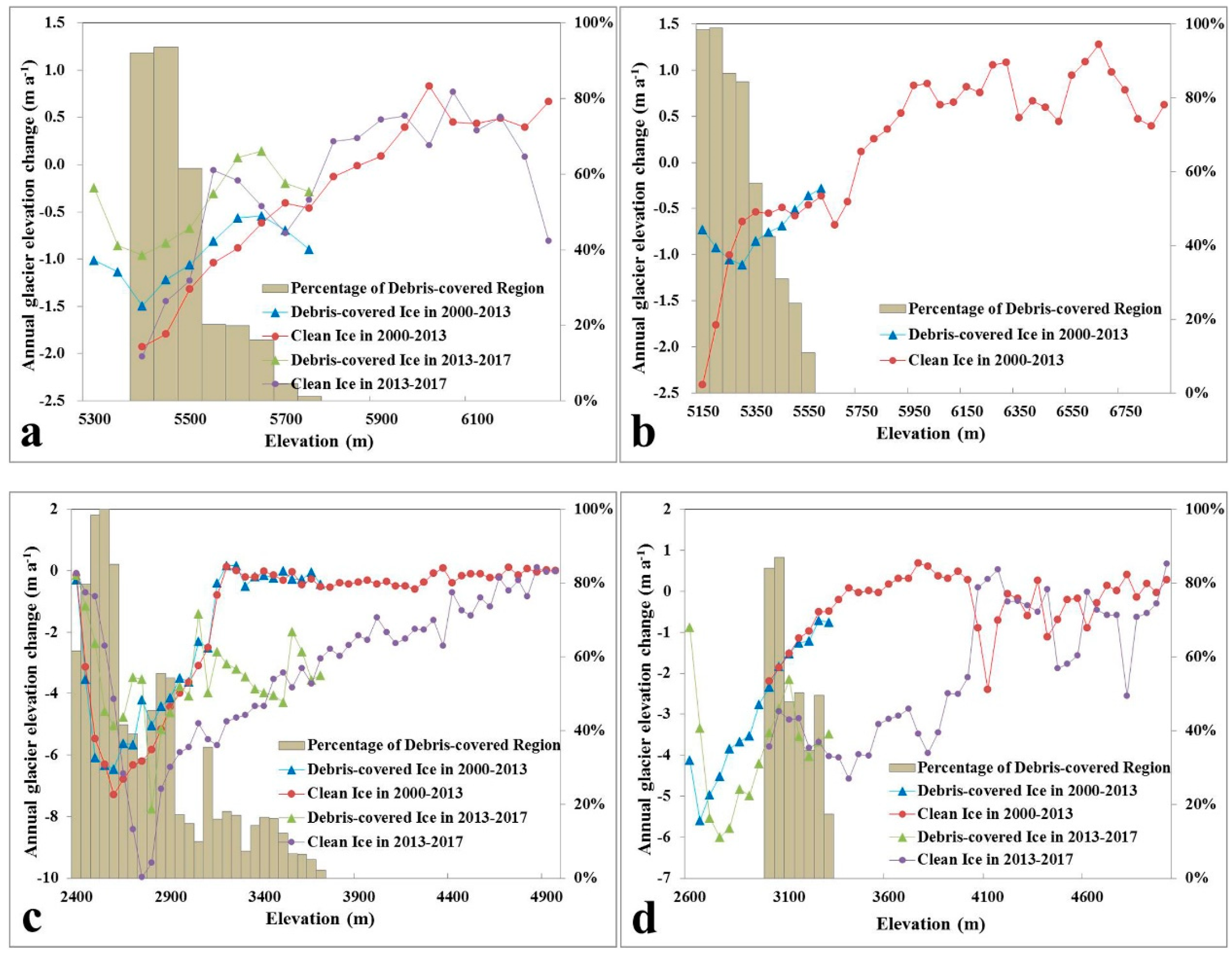
4.5. Effects of Debris on Glacier Mass Balance

The effects of debris should not be neglected even though debris-covered glaciers only occupy a small fraction of the total glacier area in our study region. We selected an unnamed glacier (G090388E30292N) and the Xibu glacier (G090598E30389N) in the WNM, the Azha glacier (G096818E29132N) and the Xueyougu glacier (G096758E29147N) in the ENM to explore and assess the debris-cove effect in the periods 2000–2013 and 2013–2017 (Figure 12). We computed the mean elevation change in 50 m elevation bins in the mixture zones of debris and clean-ice to quantitatively estimate debris influences on glacier mass balance. The debris-covered regions were located in the terminus of all the selected glaciers, with the debris-covered area being less than the clean-ice area, overall gradually decreasing with increasing elevation (Table 7 and Figure 12). In 2000–2013, the thickness of the debris-covered regions reduced faster than that of clean-ice regions in all glaciers, and this phenomenon in the WNM continued in 2013–2017, when these rates were –0.51 m a−1 and –0.46 m a−1 in the unnamed glacier, while in the ENM the debris-covered regions melted less than clean-ice regions, where these rates were –3.65 m a−1 and –4.90 m a−1 in the Azha glacier, –3.25 m a−1 and –3.54 m a−1 in the Xueyougu glacier (Table 7). This phenomenon needs to be further confirmed by analyzing more glaciers.
The analysis of the variation with altitude of glacier elevation changes in the four glaciers provided further insights on the effect of debris (Figure 12). In the mixture region of debris-covered and clean-ice, the range of glacier elevation change in WNM was smaller than that in ENM. For example, in the Xibu glacier, the largest debris-covered glacier in the WNM, the range of glacier elevation change in the debris-covered region was from –0.28 to –1.11 m a−1 in 2000–2013 and the corresponding elevation change range in the clean-ice region was from –0.46 to –2.41 m a−1 (Figure 12b). Two processes may combine to explain such difference: (1) in the lower elevation region with higher abundance of debris, the lower albedo of debris increased radiation absorption leading to heating of the debris and to radiative and convective heat transfer to the surrounding clean-ice, while the higher abundance of debris was generally associated with relatively thicker debris, which could reduce heat conduction to the underlying ice [66]; (2) at higher elevation with a smaller extent of debris; on the contrary, debris increased glacier melting possibly because the debris absorbed more radiation than absorbed by clean-ice and the thinner debris increased heat transfer to the ice underneath, increasing melt of debris-covered ice in the end. This result showed that the effect of debris on glacier mass balance was related to the fractional abundance of debris and to glacier elevation in this study area. This mechanism should be verified by other research methods, however, such as field observation and glacier mass balance modeling.

4.6. The Effect of Glacier Surface Slope on Glacier Elevation Change

It was interesting that unlike other glaciers that experienced serious mass loss in the same elevation range, only two glaciers (1 and 2 in Figure 1b and Figure 13) in the ENM remained stable or even had a slight mass increase in the glacier tongue during 2000–2013 (Figure 13). This result was consistent with Wu et al. [31], who hypothesized that the debris cover may lead to this phenomenon. This reason, however, may also relate to the glacier surface slope. First, irradiance at the glacier surface increases with increasing slope up to a sun zenith angle equal to 0°. Second, the slopes in the central part of both glaciers are steeper (the two red rectangles in Figure 13b), and may cause glacier flow velocity to increase [67,68]. The ice flow from the upstream portion of the glacier was apparently more than sufficient to balance melting in the ablation zone. This slope effect on glacier thickness change may also explain why the correlation of glacier mass balance with glacier surface slope was poor [69]. However, this hypothesis should be further validated by combining glacier mass balance and velocity data.

5. Discussion

5.1. Internal Consistency of the Glacier Elevation Change Retrieved with the ZY-3 TLA Data

The glacier elevation change in 2000–2017 can be estimated by applying two methods: one is by directly calculating the difference between the 2017 ZY−3 and the 2000 SRTM DEMs (see DEM differencing in Section 3.2), while the second one is by applying the same method separately to 2000–2013 using the 2013 ZY−3 and 2000 SRTM DEMs and to 2013–2017 using the 2017 and 2013 ZY−3 DEMs, then adding up the results. In the case of error−free data the two procedures should yield the same result. We assessed the quality of our elevation data by comparing the estimates obtained with the two procedures. In this assessment, only the pixels in the glacier elevation change maps before gap filling were used for eliminating the effect of assumptions on glacier change (see gap filling in Section 3.2). The scatter plots of the glacier thickness changes in 50 m elevation bin in 2000–2017 obtained by the two methods in both WNM and ENM show a high overall correlation (Figure 14). In the WNM, the mean thickness changes computed by the two methods were –5.10 m and –5.62 m in 2000–2017, the residual was 0.52 m and R2 was 0.9932, while in the ENM, these values were –27.71 m, −28.21 m, 0.50 m and 0.9998, respectively. The annual thickness change errors were 0.031 m a−1 (i.e., 0.026 m w.e. a−1) and 0.029 m a−1 (i.e., 0.025 m w.e. a−1), which had a limited impact on our estimates of region−wide glacier mass balance.

5.2. Cross-Comparison of ZY-3 TLA with Other Data Sources Results

Spaceborne photogrammetry and InSAR are two of the main remote sensing techniques to retrieve the high spatial resolution pattern of glacier mass balance, but it is necessary to estimate the spatial consistency of the two retrievals. In this study, we used ZY-3 TLA and TanDEM-X data to compare these two techniques. First of all, we qualitatively described the performance of ZY-3 TLA data in glacier elevation change retrieval by comparing our retrievals with TanDEM-X data (Figure 15). The result shows that high resolution ZY-3 glacier elevation change map could provide more details in some regions. We took an ice crack region in the middle of the Parlung No.4 glacier as an example to describe these detailed differences (the purple rectangle in the Figure 15a,b, the images are Gaofen-1 true color images with band 4 (R), band 3 (G) and band 2 (B) on 3 December, 2014). Although the spatial patterns of glacier elevation change in both maps were similar, the ZY-3 map showed more details in the glacier crevasses (Figure 15d), while it seems to be smoother in the TanDEM-X map (Figure 15c).
Furthermore, we compared the absolute difference of glacier elevation change derived with both data. The acquisition dates of ZY-3 TLA and TanDEM-X were 3 December 2013 and 12 March 2014 in the WNM, which were very close compared with decadal glacier elevation change and could be applied to evaluate our retrievals of glacier thickness change against an independent data source, assuming the glaciers in winter were stable during this short period. According to the snow correction of the WNM retrievals (seasonal correction in Section 3.2), this assumption is reasonable. In the ablation region, the retrievals with ZY-3 TLA (our results) and TanDEM-X (results made by Li et al. [9]) were well correlated, i.e., the R2 and slope of the regression line reached 0.99 and 0.90 (near 1.00), while the retrievals with the ZY-3 TLA data in the accumulation zone were distinctly higher than the ones with the TanDEM-X data (Figure 16). This result may have a two–fold explanation: (a) the ZY-3 results with lower valid data percentage (59.1%) in the accumulation zone had relative higher uncertainty than that in the ablation zone with higher valid data percentage (71.0%); (b) the X-band SAR signal can penetrate snow/firn in the accumulation zone, but no correction was applied when calculating glacier thickness change with the TanDEM-X and SRTM DEM data (Li et al. [9]).
According to the research of Dehecq et al. [70], the penetration depth of the X-band SAR signal may be up to 4–6 m in the accumulation zone which is covered by dry snow and/or firn. Assuming the accuracy of the glacier elevation changes retrieved from ZY-3 and TanDEM-X data was acceptable, as demonstrated by the retrievals in the ablation zone, then the penetration depth of X-band SAR signal could be estimated from the difference between the retrievals with the ZY-3 TLA (2013-12-03) and TanDEM-X (2014-03-12) data. The result showed that the mean penetration depths of X-band SAR signal could be up to 4.62 m in the accumulation zone, consistent with the value of 4–6 m documented by Dehecq et al. [70].

5.3. Comparison with Previous Studies

Firstly, we compared our results with others in some special glaciers with in-situ observations available. Thus far, in-situ measurements glacier mass balances were available on three glaciers in our study regions [35,57,58,71], i.e., the Zhadang and Gurenhekou glaciers (WNM) and the Parlung No.4 (ENM) (Table 8 and Table 9). As a whole, our results were consistent with other geodetic mass balance results, the range of difference between them is from 0.07 to 0.13 m w.e. a−1, while they were discrepant with field measurements in some periods since the timing of in-situ observations was different from our retrievals.
Secondly, the region−wide mass balance also can be calculated by applying different techniques, such as in-situ observation, ICESat/GLAS laser altimetry, photogrammetry and InSAR (Table 8 and Table 9). In the WNM, our retrievals of the mass balances gave on average –0.22 ± 0.23 m w.e. a−1, rather close to previous studies with range in –0.2 to –0.24 ± 0.13 m w.e. a−1 [5,9,72]. In the ENM our region−wide mass balance of –0.56 ± 0.20 m w.e. a−1 was similar to most published results despite large differences reported by these studies. In addition, the similarity in the time of observation and in the study area provided a good opportunity to estimate the accuracy of ZY-3 TLA and TerraSAR−X/TanDEM−X data in estimating the glacier mass balance within the entire region. The results showed that the region−wide glacier melt rate captured by ZY-3 TLA data was slightly less than that estimated with TerraSAR-X/TanDEM-X images, which may be caused by neglecting X−band SAR penetration depth as discussed in the Section 5.2. In the WNM, our results were –0.22 ± 0.23 m w.e. a−1 and –0.30 ± 0.19 m w.e. a−1 in 2000–2013 and 2000–2017, while the TerraSAR-X/TanDEM-X result in 2000–2014 was –0.24 ± 0.13 m w.e. a−1. In the ENM the mass balance was –0.56 ± 0.20 m w.e. a−1 in 2000–2017 and –0.67 ± 0.09 m w.e. a−1 during 2000–2014 from Wu et al. [31]. In addition, both previous studies [9,13,31] and our results indicated that the glaciers mass balances were different in different basins. In the WNM, for example, the mass balance differences between inside and outside the Nam Co basin were –0.049 ± 0.129 m w.e. a−1 in Li et al. [9] and –0.08 ± 0.23 m w.e. a−1 in our result. This difference may be caused by the difference in glacier orientation and glacier size between our study and Li et al. [9], since we did not evaluate exactly the same glaciers.
Moreover, the comparison of glacier mass balance in the WNM and ENM indicated the glaciers in both study regions experienced a mass loss after 2000, with a larger melt after 2013. At the same time, the glaciers in the accumulation zones remained nearly stable as shown by very small elevation change (0.05 ± 0.19 m w.e. a−1 in the WNM and 0.005 ± 0.20 m w.e. a−1 in the ENM, Table 6). On the other hand, there were clear differences in the spatial pattern of the mass balance, i.e., the mass loss rate in the ENM (–0.56 ± 0.20 m w.e. a−1) was higher than that in the WNM (–0.30 ± 0.19 m w.e. a−1) during 2000–2017.
Finally, we summarized our results and the study of Zhou et al. [3] on the glacier mass balance in the two regions during the last half century. The results showed that the mass balance patterns were clearly different in the two regions. The rate of glacier mass loss in the WNM was almost stable (~ –0.20 m w.e. a−1), while it increased in the ENM from –0.19 m w.e. a−1 before 2000 to –0.60 m w.e. a−1 after 2000 according to post-2000 studies (2000–2014 by Wu et al., 2018 and 2000–2017 by our study). This finding may suggest that effect of Indian and East Asian monsoons were weakening in this region, while the effect of Westerlies grew in the past 40 years [5].

5.4. Advantages and Disadvantages of ZY-3 TLA Data to Capture Glacier Mass Balance

ZY-3 TLA data have many advantages when retrieving the glacier mass balance. First, the sufficiently dense point cloud (3.92 m/p) makes it feasible to generate 5 m resolution DEMs, which can provide more details on spatial pattern of glacier mass balance and be references for the results of glacier models compared with the coarser resolution of many previous studies, such as 30 m spatial resolution by Burn et al. [13] and Zhou et al. [3] (Figure 7). Second, the percentage of valid data in the final glacier elevation change maps was generally higher than in some other studies, this attributes to its capability of three pairs of view angle observations. For example, the percentages of valid data in our glacier elevation change maps in 2000–2017 were 78% and 67% in the ENM and WNM, respectively, while these values in Zhou et al. [3] were 57% and 54% in the same regions using KH-9 and SRTM data.
At the same time, there are two main disadvantages in applying ZY-3 TLA data. As with other optical satellite data, cloud cover may be the primary obstacle for generating DEMs using ZY-3 data, and even very thin cloud will cause huge elevation error. In general, the percentage of cloudy days in glacier region is very high, especially in the ENM which is dominated by the monsoon climate. For instance, there are only 5 ZY-3 cloudless image data sets available in the Kangri Karpo Mountains from 2012 (launch year) to 2017. Although mosaicking data acquired at different time may mitigate this problem, some new challenges, such as time normalization and differences in glacier condition, will be introduced as well.
Since most ZY-3 cloudless images are in the winter, the snow cover is the second problem. It may affect the retrieval of glacier thickness change in many ways. First of all, the low contrast of snow surface will lead to less matching points, and then cause more DEM holes, noise and outliers in the reconstructed elevation of glacier surface. For example, the glacier surface elevation map in the ENM in 2000–2013 had only 8.62% valid values and was far less than the 77.53% in 2000–2017, because of the large snow-covered area. Moreover, the snow thickness will be mixed in the final DEM results, and this could result in significant errors when calculating DEM differences in deep snow regions, such as the Himalaya, Pamir and Southeastern Tibetan Plateau mountainous areas, where the mean snow depths were more than 0.20 m and the maximum can even reach to 0.70 m in winter [74]. This error will become larger as snow accumulates at high altitude.

6. Conclusions

In this study, we improved the DEM extraction procedure with high spatial resolution ZY-3 TLA stereo images by fusing three pairs of view angle combinations and evaluated the performance in retrieving the glacier surface elevation in the NM. Then, investigated the glacier mass balances in WNM and ENM during 2000–2017 using SRTM DEM (2000) and ZY-3 TLA stereo images (2013, 2017), as well as analyzed the spatial patterns of glacier mass balance between 2000 and 2017 in these two study areas.
By applying our improved procedure, ZY-3 TLA data did significantly increase the point cloud density and decreased invalid data on the glacier surface compared with a traditional single-pair of stereo images. We demonstrated the feasibility of generating high spatial resolution (5 m) glacier mass balance maps within several years using ZY-3 TLA data. These 5 m resolution maps can provide more details to help us better understand glacier mass balance, crevasse and other glacier properties. The terrain complexity seems to be an obstacle when retrieving glacier elevation change, while snow and cloud cover will seriously affect glacier mass balance retrievals.
The glaciers in both the WNM and ENM experienced mass loss during 2000–2017, and showed increased melt in recent years (2013–2017). The overall glacier mass balances in the WNM were –0.22 ± 0.23 m w.e. a−1, –0.43 ± 0.06 m w.e. a−1 and –0.30 ± 0.19 m w.e. a−1 in 2000–2013, 2013–2017 and 2000–2017, respectively, and the mass balance was –0.56 ± 0.20 m w.e. a−1 in 2000–2017 in the ENM. Our results also indicated that the fractional abundance of debris and glacier slope could affect the glacier mass balance. Comparisons between results with ZY-3 and TanDEM-X demonstrated that they agreed in the ablation zone, while the mean difference can reach 4.62 m in the accumulation zone because of the snow/firn penetration depth of X-band SAR signal. According to our results, a penetration correction should be applied to X-band SAR data when calculating the glacier elevation change by X−band SAR images, especially in the accumulation region.
With our improved stereo procedure applied to high spatial resolution ZY-3 TLA stereo images, accurate glacier mass balance map with high spatial resolution could be generated. At the same time, our procedure can also be applied to other TLA stereo images, such as ALOS Panchromatic Remote-sensing Instrument for Stereo Mapping (PRISM) and Pléiades to improve accuracy along with spatial and temporal sampling.

Author Contributions

Conceptualization, S.R., M.M. and L.J.; methodology, S.R. and M.M.; software, S.R.; validation, S.R.; formal analysis, S.R., L.J., M.M., J.Z. (Jing Zhang) and J.Z. (Jingxiao Zhang); investigation, S.R.; resources, L.J. and M.M.; data curation, S.R., L.J. and X.L.; writing—original draft preparation, S.R.; writing—review and editing, L.J. and M.M.; visualization, S.R.; supervision, L.J. and M.M.; project administration, L.J.; funding acquisition, L.J. and M.M. All authors have read and agreed to the published version of the manuscript.

Funding

This research was funded by the National Natural Science Foundation of China project, grant number 91737205; the Strategic Priority Research Program of the Chinese Academy of Sciences, grant numbers XDA19030203 and XDA19070102 and the MOST High Level Foreign Expert program grant number, G20190161018.

Acknowledgements

We thank USGS for freely providing SRTM-C DEM and Landsat data and DLR for free access to SRTM-X DEM. Li et al. and Wu et al. made available for this study their results of glacier elevation change retrieved by bistatic TerraSAR-X/TanDEM-X SAR images in the WNM and ENM.

Conflicts of Interest

The authors declare no conflict of interest.

References

  1. Kaser, G.; Grosshauser, M.; Marzeion, B. Contribution potential of glaciers to water availability in different climate regimes. Proc. Natl. Acad. Sci. USA 2010, 107, 20223–20227. [Google Scholar] [CrossRef] [Green Version]
  2. Wang, W.C.; Xiang, Y.; Gao, Y.; Lu, A.X.; Yao, T.D. Rapid expansion of glacial lakes caused by climate and glacier retreat in the Central Himalayas. Hydrol. Process. 2015, 29, 859–874. [Google Scholar] [CrossRef]
  3. Zhou, Y.S.; Li, Z.W.; Li, J.; Zhao, R.; Ding, X.L. Glacier mass balance in the Qinghai Tibet Plateau and its surroundings from the mid-1970s to 2000 based on Hexagon KH-9 and SRTM DEMs. Remote Sens. Environ. 2018, 210, 96–112. [Google Scholar] [CrossRef]
  4. Kaab, A.; Berthier, E.; Nuth, C.; Gardelle, J.; Arnaud, Y. Contrasting patterns of early twenty-first-century glacier mass change in the Himalayas. Nature 2012, 488, 495–498. [Google Scholar] [CrossRef] [PubMed]
  5. Yao, T.D.; Thompson, L.; Yang, W.; Yu, W.S.; Gao, Y.; Guo, X.J.; Yang, X.X.; Duan, K.Q.; Zhao, H.B.; Xu, B.Q.; et al. Different glacier status with atmospheric circulations in Tibetan Plateau and surroundings. Nat. Clim. Chang. 2012, 2, 663–667. [Google Scholar] [CrossRef]
  6. Maurer, J.M.; Schaefer, J.M.; Rupper, S.; Corley, A. Acceleration of ice loss across the Himalayas over the past 40 years. Sci. Adv. 2019, 5. [Google Scholar] [CrossRef] [Green Version]
  7. Gardelle, J.; Berthier, E.; Arnaud, Y.; Kaab, A. Region-wide glacier mass balances over the Pamir-Karakoram-Himalaya during 1999–2011 (vol 7, pg 1263, 2013). Cryosphere 2013, 7, 1885–1886. [Google Scholar] [CrossRef] [Green Version]
  8. Immerzeel, W.W.; Kraaijenbrink, P.D.A.; Shea, J.M.; Shrestha, A.B.; Pellicciotti, F.; Bierkens, M.F.P.; de Jong, S.M. High-resolution monitoring of Himalayan glacier dynamics using unmanned aerial vehicles. Remote Sens. Environ. 2014, 150, 93–103. [Google Scholar] [CrossRef]
  9. Li, G.; Lin, H. Recent decadal glacier mass balances over the Western Nyaingentanglha Mountains and the increase in their melting contribution to Nam Co Lake measured by differential bistatic SAR interferometry. Glob. Planet. Chang. 2017, 149, 177–190. [Google Scholar] [CrossRef] [Green Version]
  10. Berthier, E.; Vincent, C.; Magnusson, E.; Gunnlaugsson, A.T.; Pitte, P.; Le Meur, E.; Masiokas, M.; Ruiz, L.; Palsson, F.; Belart, J.M.C.; et al. Glacier topography and elevation changes derived from Pleiades sub-meter stereo images. Cryosphere 2014, 8, 2275–2291. [Google Scholar] [CrossRef] [Green Version]
  11. Bolch, T.; Pieczonka, T.; Benn, D.I. Multi-decadal mass loss of glaciers in the Everest area (Nepal Himalaya) derived from stereo imagery. Cryosphere 2011, 5, 349–358. [Google Scholar] [CrossRef] [Green Version]
  12. Ragettli, S.; Bolch, T.; Pellicciotti, F. Heterogeneous glacier thinning patterns over the last 40 years in Langtang Himal, Nepal. Cryosphere 2016, 10, 2075–2097. [Google Scholar] [CrossRef] [Green Version]
  13. Brun, F.; Berthier, E.; Wagnon, P.; Kaab, A.; Treichler, D. A spatially resolved estimate of High Mountain Asia glacier mass balances from 2000 to 2016. Nat. Geosci. 2017, 10, 668–673. [Google Scholar] [CrossRef] [PubMed]
  14. Rieg, L.; Klug, C.; Nicholson, L.; Sailer, R. Pleiades Tri-Stereo Data for Glacier Investigations—Examples from the European Alps and the Khumbu Himal. Remote Sens. 2018, 10, 1563. [Google Scholar] [CrossRef] [Green Version]
  15. Tian, J.; Reinartz, P.; d’Angelo, P.; Ehlers, M. Region-based automatic building and forest change detection on Cartosat-1 stereo imagery. ISPRS J. Photogramm. Remote Sens. 2013, 79, 226–239. [Google Scholar] [CrossRef]
  16. Qin, R.J. Change detection on LOD 2 building models with very high resolution spaceborne stereo imagery. ISPRS J. Photogramm. Remote Sens. 2014, 96, 179–192. [Google Scholar] [CrossRef]
  17. Al-Rawabdeh, A.; He, F.N.; Moussa, A.; El-Sheimy, N.; Habib, A. Using an Unmanned Aerial Vehicle-Based Digital Imaging System to Derive a 3D Point Cloud for Landslide Scarp Recognition. Remote Sens. 2016, 8, 95. [Google Scholar] [CrossRef] [Green Version]
  18. Dall’Asta, E.; Forlani, G.; Roncella, R.; Santise, M.; Diotri, F.; di Cella, U.M. Unmanned Aerial Systems and DSM matching for rock glacier monitoring. ISPRS J. Photogramm. Remote Sens. 2017, 127, 102–114. [Google Scholar] [CrossRef]
  19. Meng, X.; Wang, L.; Silván-Cárdenas, J.L.; Currit, N. A multi-directional ground filtering algorithm for airborne LIDAR. ISPRS J. Photogramm. Remote Sens. 2009. [Google Scholar] [CrossRef] [Green Version]
  20. Mongus, D.; Žalik, B. Parameter-free ground filtering of LiDAR data for automatic DTM generation. ISPRS J. Photogramm. Remote Sens. 2012. [Google Scholar] [CrossRef]
  21. Skinner, B.; Vidal-Calleja, T.; Miro, J.V.; De Bruijn, F.; Falque, R. 3D point cloud upsampling for accurate reconstruction of dense 2.5 D thickness maps. In Proceedings of the Australasian Conference on Robotics and Automation, ACRA, Melbourne, Australia, 2–4 December 2014. [Google Scholar]
  22. Liu, S.; Yao, X.; Guo, W.; Junli, X.U.; Shangguan, D.; Wei, J.; Bao, W.; Lizong, W.U. The contemporary glaciers in China based on the Second Chinese Glacier Inventory. Acta Geogr. Sin. 2015, 70, 3–16. [Google Scholar]
  23. Zhou, S.; Kang, S.; Chen, F.; Joswiak, D.R. Water balance observations reveal significant subsurface water seepage from Lake Nam Co, south-central Tibetan Plateau. J. Hydrol. 2013, 491, 89–99. [Google Scholar] [CrossRef]
  24. Lei, Y.; Yao, T.; Bird, B.W.; Yang, K.; Zhai, J.; Sheng, Y. Coherent lake growth on the central Tibetan Plateau since the 1970s: Characterization and attribution. J. Hydrol. 2013, 483, 61–67. [Google Scholar] [CrossRef]
  25. Wu, B.Y. Weakening of Indian summer monsoon in recent decades. Adv. Atmos. Sci. 2005, 22, 21–29. [Google Scholar]
  26. Lin, H.; Li, G.; Cuo, L.; Hooper, A.; Ye, Q.H. A decreasing glacier mass balance gradient from the edge of the Upper Tarim Basin to the Karakoram during 2000–2014. Sci. Rep. 2017, 7. [Google Scholar] [CrossRef]
  27. Gautam, R.; Hsu, N.C.; Lau, W.K.M.; Yasunari, T.J. Satellite observations of desert dust-induced Himalayan snow darkening. Geophys. Res. Lett. 2013, 40, 988–993. [Google Scholar] [CrossRef] [Green Version]
  28. Ming, J.; Wang, Y.; Du, Z.; Zhang, T.; Guo, W.; Xiao, C.; Xu, X.; Ding, M.; Zhang, D.; Yang, W. Widespread albedo decreasing and induced melting of Himalayan snow and ice in the early 21st century. PLoS ONE 2015, 10. [Google Scholar] [CrossRef] [Green Version]
  29. Kodamana, R.; Gautam, R. Light absorbing impurity deposition over the Himalayan-Karakoram-Hindu Kush-Tibetan cryosphere: A review and satellite-based characterization. L. Surf. Cryosph. Remote Sens. III 2016. [Google Scholar] [CrossRef]
  30. Li, C.; Bosch, C.; Kang, S.; Andersson, A.; Chen, P.; Zhang, Q.; Cong, Z.; Chen, B.; Qin, D.; Gustafsson, Ö. Sources of black carbon to the Himalayan-Tibetan Plateau glaciers. Nat. Commun. 2016, 7, 1–7. [Google Scholar] [CrossRef]
  31. Wu, K.; Liu, S.; Jiang, Z.; Xu, J.; Wei, J.; Guo, W. Recent glacier mass balance and area changes in the Kangri Karpo Mountains from DEMs and glacier inventories. Cryosphere 2018, 12, 103–121. [Google Scholar] [CrossRef] [Green Version]
  32. Qu, B.; Ming, J.; Kang, S.C.; Zhang, G.S.; Li, Y.W.; Li, C.D.; Zhao, S.Y.; Ji, Z.M.; Cao, J.J. The decreasing albedo of the Zhadang glacier on western Nyainqentanglha and the role of light-absorbing impurities. Atmos. Chem. Phys. 2014, 14, 11117–11128. [Google Scholar] [CrossRef] [Green Version]
  33. Kaab, A.; Treichler, D.; Nuth, C.; Berthier, E. Brief Communication: Contending estimates of 2003-2008 glacier mass balance over the Pamir-Karakoram-Himalaya. Cryosphere 2015, 9, 557–564. [Google Scholar] [CrossRef] [Green Version]
  34. Paul, F.; Bolch, T.; Kaab, A.; Nagler, T.; Nuth, C.; Scharrer, K.; Shepherd, A.; Strozzi, T.; Ticconi, F.; Bhambri, R.; et al. The glaciers climate change initiative: Methods for creating glacier area, elevation change and velocity products. Remote Sens. Environ. 2015, 162, 408–426. [Google Scholar] [CrossRef] [Green Version]
  35. Yu, W.S.; Yao, T.D.; Kang, S.C.; Pu, J.C.; Yang, W.; Gao, T.G.; Zhao, H.B.; Zhou, H.; Li, S.H.; Wang, W.C.; et al. Different region climate regimes and topography affect the changes in area and mass balance of glaciers on the north and south slopes of the same glacierized massif (the West Nyainqentanglha Range, Tibetan Plateau). J. Hydrol. 2013, 495, 64–73. [Google Scholar] [CrossRef]
  36. Bolch, T.; Yao, T.; Kang, S.; Buchroithner, M.F.; Scherer, D.; Maussion, F.; Huintjes, E.; Schneider, C. A glacier inventory for the western Nyainqentanglha Range and the Nam Co Basin, Tibet, and glacier changes 1976–2009. Cryosphere 2010, 4, 419–433. [Google Scholar] [CrossRef] [Green Version]
  37. Yao, T.D.; Li, Z.G.; Yang, W.; Guo, X.J.; Zhu, L.P.; Kang, S.C.; Wu, Y.H.; Yu, W.S. Glacial distribution and mass balance in the Yarlung Zangbo river and its influence on lakes. Chin. Sci. Bull. 2010. [Google Scholar] [CrossRef]
  38. Guo, W.Q.; Liu, S.Y.; Xu, L.; Wu, L.Z.; Shangguan, D.H.; Yao, X.J.; Wei, J.F.; Bao, W.J.; Yu, P.C.; Liu, Q.; et al. The second Chinese glacier inventory: Data, methods and results. J. Glaciol. 2015, 61, 357–372. [Google Scholar] [CrossRef] [Green Version]
  39. Wang, T.Y.; Zhang, G.; Li, D.R.; Tang, X.M.; Jiang, Y.H.; Pan, H.B.; Zhu, X.Y.; Fang, C. Geometric Accuracy Validation for ZY-3 Satellite Imagery. IEEE Geosci. Remote Sens. Lett. 2014, 11, 1168–1171. [Google Scholar] [CrossRef]
  40. Ni, W.J.; Sun, G.Q.; Ranson, K.J.; Pang, Y.; Zhang, Z.Y.; Yao, W. Extraction of ground surface elevation from ZY-3 winter stereo imagery over deciduous forested areas. Remote Sens. Environ. 2015, 159, 194–202. [Google Scholar] [CrossRef]
  41. Zhou, P.; Tang, X.; Wang, Z.; Cao, N.; Wang, X. Vertical accuracy effect verification for satellite imagery with different GCPs. IEEE Geosci. Remote Sens. Lett. 2017, 14, 1268–1272. [Google Scholar] [CrossRef]
  42. Bhardwaj, A.; Sam, L.; Martin-Torres, F.J.; Kumar, R. UAVs as remote sensing platform in glaciology: Present applications and future prospects. Remote Sens. Environ. 2016, 175, 196–204. [Google Scholar] [CrossRef]
  43. Berthier, E.; Schiefer, E.; Clarke, G.K.C.; Menounos, B.; Remy, F. Contribution of Alaskan glaciers to sea-level rise derived from satellite imagery. Nat. Geosci. 2010, 3, 92–95. [Google Scholar] [CrossRef] [Green Version]
  44. Berthier, E.; Arnaud, Y.; Baratoux, D.; Vincent, C.; Remy, F. Recent rapid thinning of the “Mer de Glace” glacier derived from satellite optical images. Geophys. Res. Lett. 2004, 31. [Google Scholar] [CrossRef] [Green Version]
  45. King, O.; Quincey, D.J.; Carrivick, J.L.; Rowan, A. V Spatial variability in mass loss of glaciers in the Everest region, central Himalayas, between 2000 and 2015. Cryosphere 2017, 11, 407–426. [Google Scholar] [CrossRef] [Green Version]
  46. Nuth, C.; Kaab, A. Co-registration and bias corrections of satellite elevation data sets for quantifying glacier thickness change. Cryosphere 2011, 5, 271–290. [Google Scholar] [CrossRef] [Green Version]
  47. Pieczonka, T.; Bolch, T.; Wei, J.F.; Liu, S.Y. Heterogeneous mass loss of glaciers in the Aksu-Tarim Catchment (Central Tien Shan) revealed by 1976 KH-9 Hexagon and 2009 SPOT-5 stereo imagery. Remote Sens. Environ. 2013, 130, 233–244. [Google Scholar] [CrossRef] [Green Version]
  48. Hohle, J.; Hohle, M. Accuracy assessment of digital elevation models by means of robust statistical methods. ISPRS J. Photogramm. Remote Sens. 2009, 64, 398–406. [Google Scholar] [CrossRef] [Green Version]
  49. Neelmeijer, J.; Motagh, M.; Bookhagen, B. High-resolution digital elevation models from single-pass TanDEM-X interferometry over mountainous regions: A case study of Inylchek Glacier, Central Asia. ISPRS J. Photogramm. Remote Sens. 2017, 130, 108–121. [Google Scholar] [CrossRef] [Green Version]
  50. Ke, L.; Ding, X.; Zhang, L.; Hu, J.; Shum, C.K.; Lu, Z. Compiling a new glacier inventory for southeastern Qinghai-Tibet Plateau from Landsat and Palsar data. J. Glaciol. 2016, 62, 579–592. [Google Scholar] [CrossRef] [Green Version]
  51. Paul, F.; Barrand, N.E.; Baumann, S.; Berthier, E.; Bolch, T.; Casey, K.; Frey, H.; Joshi, S.P.; Konovalov, V.; Le Bris, R.; et al. On the accuracy of glacier outlines derived from remote-sensing data. Ann. Glaciol. 2013, 54, 171–182. [Google Scholar] [CrossRef] [Green Version]
  52. Dussaillant, I.; Berthier, E.; Brun, F.; Masiokas, M.; Hugonnet, R.; Favier, V.; Rabatel, A.; Pitte, P.; Ruiz, L. Two decades of glacier mass loss along the Andes. Nat. Geosci. 2019, 12, 802–808. [Google Scholar] [CrossRef]
  53. Huintjes, E.; Sauter, T.; Schroter, B.; Maussion, F.; Yang, W.; Kropaček, J.; Buchroithner, M.; Scherer, D.; Kang, S.; Schneider, C. Evaluation of a Coupled Snow and Energy Balance Model for Zhadang Glacier, Tibetan Plateau, Using Glaciological Measurements and Time-Lapse Photography. Arct. Antarct. Alp. Res. 2015, 47, 573–590. [Google Scholar] [CrossRef]
  54. Zhou, Y.S.; Li, Z.; Li, J. Slight glacier mass loss in the Karakoram region during the 1970s to 2000 revealed by KH-9 images and SRTM DEM. J. Glaciol. 2017, 63, 331–342. [Google Scholar] [CrossRef] [Green Version]
  55. Rignot, E.; Echelmeyer, K.; Krabill, W. Penetration depth of interferometric synthetic-aperture radar signals in snow and ice. Geophys. Res. Lett. 2001, 28, 3501–3504. [Google Scholar] [CrossRef] [Green Version]
  56. Dall, J.; Madsen, S.N.; Keller, K.; Forsberg, R. Topography and penetration of the greenland ice sheet measured with airborne SAR interferometry. Geophys. Res. Lett. 2001, 28, 1703–1706. [Google Scholar] [CrossRef]
  57. Zhang, G.S.; Kang, S.C.; Fujita, K.; Huintjes, E.; Xu, J.Q.; Yamazaki, T.; Haginoya, S.; Wei, Y.; Scherer, D.; Schneider, C.; et al. Energy and mass balance of Zhadang glacier surface, central Tibetan Plateau. J. Glaciol. 2013, 59, 137–148. [Google Scholar] [CrossRef] [Green Version]
  58. Yang, W.; Yao, T.D.; Xu, B.Q.; Wu, G.J.; Ma, L.L.; Xin, X.D. Quick ice mass loss and abrupt retreat of the maritime glaciers in the Kangri Karpo Mountains, southeast Tibetan Plateau. Chin. Sci. Bull. 2008, 53, 2547–2551. [Google Scholar] [CrossRef] [Green Version]
  59. Huss, M. Density assumptions for converting geodetic glacier volume change to mass change. Cryosphere 2013, 7, 877–887. [Google Scholar] [CrossRef] [Green Version]
  60. Shangguan, D.H.; Bolch, T.; Ding, Y.J.; Krohnert, M.; Pieczonka, T.; Wetzel, H.U.; Liu, S.Y. Mass changes of Southern and Northern Inylchek Glacier, Central Tian Shan, Kyrgyzstan, during similar to 1975 and 2007 derived from remote sensing data. Cryosphere 2015, 9, 703–717. [Google Scholar] [CrossRef] [Green Version]
  61. Koblet, T.; Gartner-Roer, I.; Zemp, M.; Jansson, P.; Thee, P.; Haeberli, W.; Holmlund, P. Reanalysis of multi-temporal aerial images of Storglaciaren, Sweden (1959–99)—Part 1: Determination of length, area, and volume changes. Cryosphere 2010, 4, 333–343. [Google Scholar] [CrossRef] [Green Version]
  62. Neckel, N.; Braun, A.; Kropacek, J.; Hochschild, V. Recent mass balance of the Purogangri Ice Cap, central Tibetan Plateau, by means of differential X-band SAR interferometry. Cryosphere 2013, 7, 1623–1633. [Google Scholar] [CrossRef] [Green Version]
  63. Xu, K.; Jiang, Y.; Zhang, G.; Zhang, Q.; Wang, X. Geometric potential assessment for ZY3-02 triple linear array imagery. Remote Sens. 2017, 9, 658. [Google Scholar] [CrossRef] [Green Version]
  64. Grohmann, C.H. Evaluation of TanDEM-X DEMs on selected Brazilian sites: Comparison with SRTM, ASTER GDEM and ALOS AW3D30. Remote Sens. Environ. 2018, 212, 121–133. [Google Scholar] [CrossRef] [Green Version]
  65. Neckel, N.; Loibl, D.; Rankl, M. Recent slowdown and thinning of debris-covered glaciers in south-eastern Tibet. Earth Planet. Sci. Lett. 2017, 464, 95–102. [Google Scholar] [CrossRef] [Green Version]
  66. Huang, L.; Li, Z.; Han, H.; Tian, B.; Zhou, J. Analysis of thickness changes and the associated driving factors on a debris-covered glacier in the Tienshan Mountain. Remote Sens. Environ. 2018. [Google Scholar] [CrossRef]
  67. Cuffey, K.M.; Paterson, W.S.B. The Physics of Glaciers, 4th ed.; Elsevier: Burlington, MA, USA, 2010; ISBN 9780123694614. [Google Scholar]
  68. Muller, J.; Vieli, A.; Gartner-Roer, I. Rock glaciers on the run-understanding rock glacier landform evolution and recent changes from numerical flow modeling. Cryosphere 2016, 10, 2865–2886. [Google Scholar] [CrossRef] [Green Version]
  69. Lin, L.; Jiang, L.; Sun, Y.; Yi, C.; Wang, H.; Hsu, H. Glacier elevation changes (2012–2016) of the Puruogangri Ice Field on the Tibetan Plateau derived from bi-temporal TanDEM-X InSAR data. Int. J. Remote Sens. 2016, 37, 5687–5707. [Google Scholar]
  70. Dehecq, A.; Millan, R.; Berthier, E.; Gourmelen, N.; Trouve, E.; Vionnet, V. Elevation Changes Inferred From TanDEM-X Data Over the Mont-Blanc Area: Impact of the X-Band Interferometric Bias. Ieee J. Sel. Top. Appl. Earth Obs. Remote Sens. 2016, 9, 3870–3882. [Google Scholar] [CrossRef] [Green Version]
  71. Zhang, G.S.; Kang, S.C.; Cuo, L.; Qu, B. Modeling hydrological process in a glacier basin on the central Tibetan Plateau with a distributed hydrology soil vegetation model. J. Geophys. Res. 2016, 121, 9521–9539. [Google Scholar] [CrossRef] [Green Version]
  72. Neckel, N.; Kropacek, J.; Bolch, T.; Hochschild, V. Glacier mass changes on the Tibetan Plateau 2003-2009 derived from ICESat laser altimetry measurements. Environ. Res. Lett. 2014, 9. [Google Scholar] [CrossRef]
  73. Gardner, A.S.; Moholdt, G.; Cogley, J.G.; Wouters, B.; Arendt, A.A.; Wahr, J.; Berthier, E.; Hock, R.; Pfeffer, W.T.; Kaser, G.; et al. A Reconciled Estimate of Glacier Contributions to Sea Level Rise: 2003 to 2009. Science 2013, 340, 852–857. [Google Scholar] [CrossRef] [PubMed] [Green Version]
  74. Dai, L.Y.; Che, T.; Xie, H.J.; Wu, X.J. Estimation of Snow Depth over the Qinghai-Tibetan Plateau Based on AMSR-E and MODIS Data. Remote Sens. 2018, 10, 1989. [Google Scholar] [CrossRef] [Green Version]
Figure 1. Overview of the study areas, (a): Western Nyainqentanglha Mountains (WNM); (b): Eastern Nyainqentanglha Mountains (ENM). The green rectangles and characters represent the coverage and acquisition time of ZiYuan-3 Three-Line-Array (ZY-3 TLA) data, the yellow polygons represent the glacier outlines, the black and green points represent sample glaciers and the thick black lines are the boundaries of the basins. (Background: Sentinel 2A false color images of band 11 (SWIR), band 8 (NIR), band 4 (R) shown in red, green, blue composition).
Remotesensing 12 00864 g001
Figure 2. Workflow applied to generate the ZY-3 DEM and to estimate the glacier mass balance.
Remotesensing 12 00864 g002
Figure 3. Variability of the elevation difference (dh) standardized by the tangent of slope (α) with aspect (φ) in different co-registration combinations: (a) 2017NBENM—SRTM-C; (b): 2017NFENM—SRTM-C; (c) 2017BFENM—SRTM-C. The ZY-3 DEM was registered to the SRTM-C DEM. The red line shows the corresponding fitting function as defined by Equation (3).
Remotesensing 12 00864 g003
Figure 4. One example of ELA extraction in the central WNM. The base map is Landsat TM false color images of band 5, band 4 and band 2 shown in red, green and blue composition on 20070708.
Remotesensing 12 00864 g004
Figure 5. Penetration depth (expressed by the mean ± standard deviation) estimated as the difference between SRTM-X and SRTM-C DEMs in each 50 m elevation bin in the study area: (a) WNM and (b) ENM; clean and debris-covered glaciers in the ENM delineated as described in the glacier mapping part in Section 3.2.
Remotesensing 12 00864 g005
Figure 6. The point cloud of the Parlung No.4 glacier derived by ZY-3 TLA data. (a) The overview of the Parlung No.4 glacier (The basemap is the same as in Figure 1b); (b): The point cloud generated with the one pair (NB) combination; (c) The point cloud obtained by fusing the NB (red points), NF (green points) and BF (blue points) observations.
Remotesensing 12 00864 g006
Figure 7. The percentage of valid data in the glacier elevation change maps and glacier area versus elevation in the both study areas (a) WNM; (b) ENM.
Remotesensing 12 00864 g007
Figure 8. Annual glacier elevation changes in the WNM. (a): 2000–2013; (b): 2013–2017; (c): 2000–2017; (d): Annual glacier elevation change versus elevation (the dotted black line is the zero mass balance line, the orange and purple solid vertical lines represent the ELA lines in the 2000–2013 and 2013–2017, respectively). The purple rectangle in the images is the sample glacier described in the Figure 9.
Remotesensing 12 00864 g008
Figure 9. Annual elevation changes of unnamed glacier (GLIMs ID: G090550E30416N, the purple rectangle region in Figure 8). (a): 2000–2013; (b): 2013–2017; (c): 2000–2017; (d): annual glacier elevation changes versus elevation.
Remotesensing 12 00864 g009
Figure 10. Annual glacier elevation change in the ENM. (a): 2000–2013; (b): 2013–2017; (c): 2000–2017; (d): Annual glacier elevation change versus elevation in 2000–2017. The purple rectangle is the sample glaciers described in Figure 11.
Remotesensing 12 00864 g010
Figure 11. Annual elevation changes of the Xueyougu glacier and the Azha glacier (the purple rectangle region in Figure 10). (a): 2000–2013; (b): 2013–2017; (c): 2000–2017; (d) and (e): annual glacier elevation changes of the Xueyougu glacier (d) and the Azha glacier (e) versus elevation.
Remotesensing 12 00864 g011
Figure 12. The annual elevation changes of unnamed (a), Xibu (b), Azha (c) and Xueyougu (d) in debris-covered and debris-free glaciers during 2000–2013 and 2013–2017. Note: the percentage of debris-covered region was calculated as debris area divided by the total area in each elevation bin.
Remotesensing 12 00864 g012
Figure 13. The glacier surface elevation change in 2000–2013 (a) and glacier surface slope (b) of the two sample glaciers (same with number 1 and 2 glaciers in the Figure 1b). Our reference DEM is SRTM DEM and the slope calculated by SRTM DEM using ArcMap 10.2 software approximately represents glacier surface slope in 2000–2013.
Remotesensing 12 00864 g013
Figure 14. Cross-validation of the glacier elevation changes generated by the two methods in the WNM (a) and ENM (b).
Remotesensing 12 00864 g014
Figure 15. The detail comparison of glacier elevation change derived by TanDEM-X and ZY-3 TLA data for the Parlung No.4 glacier. (a): overview of the Parlung No.4 glacier (the basemap is the 8 m spatial resolution Gaofen-1 true color image with band 4 (R), band 3 (G) and band 2 (B) composition on 3 December, 2014); (b): zoom figure of the sample region; (c) and (d): the annual glacier elevation change derived by TanDEM-X in 2000–2014 and ZY-3 TLA data in 2000–2017; their spatial resolutions are 10 m and 5 m, respectively.
Remotesensing 12 00864 g015
Figure 16. Glacier thickness changes in 50 m elevation bins from ZY-3 (02/2000–12/2013) against that from TanDEM-X (02/2000–03/2014) in the WNM.
Remotesensing 12 00864 g016
Table 1. Input and reference datasets used in this paper.
Data SourceTimeSpatial Resolution (m)Purpose
ZY-3/TLA in the Western Nyainqentanglha Mountains (WNM)2017/01/22
2013/12/03
Nadir (2.5)
Forward (3.5)
Backward (3.5)
Calculate glacier surface elevation in WNM
ZY-3/TLA in the Eastern Nyainqentanglha Mountains (ENM)2017/12/04
2013/03/09
Calculate glacier surface elevation in ENM
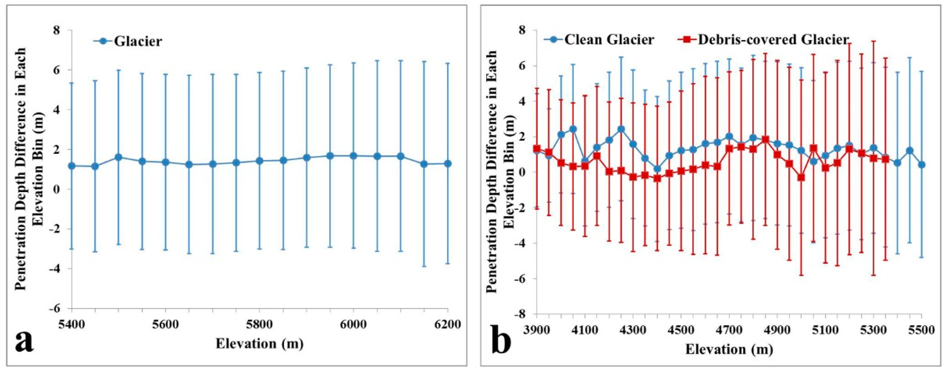
Glacier Elevation Change Maps in the WNM and ENM [9,31]2000–201410Cross-validate the ZY-3 result and estimate X-band SAR signal penetration depth into glacier surface
C-band Digital Elevation Model of Shuttle Radar Topography Mission (SRTM-C DEM)2000/0230Reference elevation both on glacier surface in 2000 and in off-glacier region
X-band Digital Elevation Model of Shuttle Radar Topography Mission (SRTM-X DEM)2000/0230Estimate C-band SAR signal penetration depth
Landsat Thematic Mapper (TM)2000–201730Classify the clean ice and debris-covered glacier
Table 2. Triangulation information for all image view angle combinations in ERDAS IMAGINE 2015. ID is expressed by year, view angle combination and study area (ENM or WNM).
IDNumber of GCPsNumber of ECPsRMSE (pixel)RMSE (m)
xyz
2017NBENM159860.501.772.461.05
2017NFENM0.531.912.211.07
2017BFENM0.701.231.902.25
2013NBENM138550.491.851.221.01
2013NFENM0.501.560.991.04
2013BFENM0.631.511.282.02
2017NBWNM1021590.291.031.820.59
2017NFWNM0.280.921.570.59
2017BFWNM0.421.121.991.36
2013NBWNM1020660.281.772.260.58
2013NFWNM0.271.81.890.55
2013BFWNM0.401.561.991.30
Mean 0.441.501.801.12
Table 3. Co-registration shifts of the ZY-3 DEMs with respect to the SRTM-C DEM and statistics on elevation difference (dh) between ZY-3 DEMs and the SRTM-C DEM in off-glacier samples with and without correction using co-registration; σ and Normalized Median Absolute Deviation (NMAD) are the standard deviation and normalized median absolute deviation of the elevation difference (dh), respectively.
IDCo-Registration Shift (m)Basic Statistics on Elevation Difference between ZY-3 DEMs and SRTM-C DEM
Before CorrectionAfter CorrectionChange in σ (%) after CorrectionChange in NMAD (%) after Correction
xyzMean ± σMedian ± NMADMean ± σMedian ± NMAD
2017NBENM3.65 2.06 1.40 −2.12 ± 9.76 −2.29 ± 8.96−0.72 ± 9.76−0.89 ± 8.960.010.01
2017NFENM4.46 1.84 6.46 −6.76 ± 9.94 −6.92 ± 9.19 −0.23 ± 9.42−0.40 ± 8.67 −5.19−5.64
2017BFENM6.25 1.88 5.30 −4.61 ± 8.81 −4.71 ± 8.04 −0.19 ± 8.49−0.10 ± 7.72 −3.69−4.07
2013NBENM3.39 5.47 −0.48 0.48 ± 11.98 0.47 ± 10.88 −0.37 ± 12.07−0.42 ± 10.96 0.730.70
2013NFENM1.89 3.25 3.73 −4.14 ± 12.83 −4.18 ± 11.75 −0.63 ± 12.07−0.74 ± 11.00 −5.91−6.40
2013BFENM5.27 5.29 2.86 −1.39 ± 9.80−1.48 ± 8.860.35 ± 9.240.44 ± 8.28 −5.63−6.45
2017NBWNM0.88 5.47 2.31 −1.74 ± 8.52−1.78 ± 5.170.35 ± 8.500.33 ± 5.15−0.22−0.27
2017NFWNM0.68 1.70 6.63 −6.91 ± 8.68−6.68 ± 5.43−0.49 ± 8.49−0.3 ± 5.32−2.19−1.85
2017BFWNM1.29 9.02 4.51 −3.87 ± 9.19−3.92 ± 5.65−0.06 ± 8.680.02 ± 5.31−5.52−5.96
2013NBWNM3.05 8.74 2.72 −1.96 ± 7.59−1.98 ± 4.710.41 ± 7.670.37 ± 4.841.092.80
2013NFWNM−1.43 9.48 6.79 −6.81 ± 7.68−6.57 ± 4.93−0.35 ± 7.33−0.19 ± 4.64−4.50−5.92
2013BFWNM−0.81 12.26 4.76 −4.01 ± 8.01−4.01 ± 5.14−0.24 ± 7.58−0.07 ± 4.74−5.35−7.80
Table 4. Mean point distance and percentage of valid data before and after fusion of the point clouds from three view angle pairs generated with the ZY-3 TLA image data. Improvement in distance is given by the distance difference between after and before fusing the point clouds, improvement in valid data is calculated by the percentage difference between after and before fusing the DEM.
IDMean Point Distance (m)Improvement in DistancePercentage of Valid Data (%)Improvement in Valid Data (%)
Before FusionAfter FusionBefore FusionAfter Fusion
2017NBENM5.053.09−1.9665.94%92.75%26.82%
2017NFENM4.24−1.1588.48%4.27%
2017BFENM9.96−6.8637.55%55.20%
2013NBENM7.744.89−2.8534.82%54.66%19.84%
2013NFENM6.82−1.9344.36%10.30%
2013BFENM15.53−10.6417.96%36.70%
2017NBWNM5.983.79−2.1968.15%85.46%17.31%
2017NFWNM5.63−1.8474.99%10.47%
2017BFWNM11.38−7.5943.51%41.95%
2013NBWNM5.863.90−1.9674.85%91.62%16.77%
2013NFWNM5.51−1.6182.57%9.05%
2013BFWNM10.90−7.0048.67%42.95%
Average7.883.92−3.9656.82%81.12%24.30%
Table 5. Vertical errors in the elevation change represented by the statistics over the off-glacier region (Ms, δ s , Median and NMAD) and estimated uncertainties in glacier elevation change and mass balance. The final residuals between DEMs were set as systematic errors in the latter error assessment. Time of acquisition is expressed by the indicated year combined with a study area (ENM or WNM). Symbols M s , δ s , N, N eff , δ e , δ mb were defined in the accuracy assessment in Section 3.2. Note that the δ mb in 2000–2013 and 2013–2017 in the ENM were not calculated because the glacier mass balance in 2013 was not retrieved (Section 4.4).
AcquisitionMs (m)δs (m)Median (m)NMAD (m)NNeffδe (m)δmb (m w.e.)
2013WNM − SRTM0.977.121.044.2881,654,7682,041,3690.970.23
2017WNM − 2013WNM0.033.040.103.0167,949,8091,698,7450.030.06
2017WNM − SRTM0.808.060.864.7368,836,8531,720,9210.800.19
2013ENM − SRTM−0.4111.12−0.5210.0756,358,7881,408,9700.41/
2017ENM − 2013ENM−0.185.95−0.294.9547,187,8721,179,6970.18/
2017ENM − SRTM−0.558.79−0.748.0062,405,1341,560,1280.550.20
Table 6. Area and mass balance (unit: m w.e. a−1) of glaciers in the WNM and ENM from 2000 to 2017. The Relative Change (RC) represents glacier relative change. Yanong glacier was excluded when calculating region-wide glacier mass balance in the ENM because of incomplete coverage by our data.
RegionWNM (m w.e. a−1)ENM (m w.e. a−1)
Area (km2)2000−20132013−2017RC (%)2000−2017Area (km2)2000−2017
Ablation region269.95−0.50 ± 0.23−0.64 ± 0.0626.8−0.55 ± 0.19403.47−0.77 ± 0.20
Accumulation region201.320.17 ± 0.23−0.16 ± 0.06192.30.05 ± 0.19148.981 0.005 ± 0.20
Inside Nam Co basin108.59−0.28 ± 0.23−0.46 ± 0.0665.6−0.32 ± 0.19
Outside Nam Co basin362.68−0.20 ± 0.23−0.41 ± 0.06106.7−0.29 ± 0.19
5O282B basin 197.23−0.52 ± 0.20
5O291B basin 355.21−0.57 ± 0.20
Total471.27−0.22 ± 0.23−0.43 ± 0.06101.8−0.30 ± 0.19552.44−0.56 ± 0.20
1 The mass balance in the accumulation region in the ENM is rounded-off to three decimal digits for clear expression.
Table 7. The surface elevation changes of the four debris-covered glaciers. Note: the area was a mixture of debris-covered and clean-ice portions; the surface elevation change of the Xibu glacier in 2013–2017 was not retrieved since cloud cover in the 2017 ZY-3 stereo images.
Glacier NameGLIMs IDRegionElevation of Mixed Region (m)Area (km2)Surface Elevation Changes (m a−1)
2000−20132013−2017
Un−namedG090388E30292NDebris-covered5400–58000.64−0.90−0.51
Clean-ice2.32−0.62−0.46
XibuG090598E30389NDebris-covered5150−56003.22−0.81/
Clean-ice3.53−0.54/
AzhaG096818E29132NDebris-covered2400−37503.01−3.40−3.65
Clean-ice6.41−1.58−4.90
XueyouguG096758E29147NDebris-covered3000−33000.96−1.53−3.25
Clean-ice1.25−0.98−3.54
Table 8. Comparison of our geodetic glacier mass balance retrievals with previous studies in the WNM.
RegionStudyDataPeriodMass Balance (m w.e. a−1)
ZhadangYu et al. [35]In-situ 2005−2008−0.59
Zhang et al. [57]In−situ2009−2011−1.20
Zhang et al. [71]In−situ2011−2014−1.60
Li et al. [9]TerraSAR-X/TanDEM-X2000−2014−0.501 ± 0.166
This studyZY-3 TLA2000−2017−0.60 ±0.19
GurenhekouYao et al. [5]In-situ 2005−2010−0.31
Yu et al. [37]In-situ 2004−2005−0.4
Li et al. [9]TerraSAR-X/TanDEM-X2000−2014−0.267 ± 0.248
This studyZY-3 TLA2000−2017−0.40 ± 0.19
Western Nyainqentanglha Mountains Yao et al. [5]In-situ 2005−2010−0.2
Neckel et al. [72]1ICESat/GLAS2003−2009−0.20 ± 0.29
Li et al. [9]TerraSAR-X/TanDEM-X2000−2014−0.235 ± 0.127
2Brun et al. [13]ASTER Stereo Image2000−2016−0.35 ± 0.07
Zhou et al. [3]KH−91975−2000−0.25 ± 0.15
This studyZY-3 TLA2000−2013−0.22 ± 0.23
2013−2017−0.43 ± 0.06
2000−2017−0.30 ± 0.19
1 where the abbreviation represents a satellite and its data named Ice, Cloud and land Elevation Satellite/Geoscience Laser Altimeter System; 2 Where the glacier mass balance of Brun et al. (2017) was recalculated with our glacier outline in our study areas.
Table 9. Comparison of our geodetic glacier mass balance retrievals with previous with studies in the ENM.
RegionStudyDataPeriodMass Balance(m w.e. a−1)
Parlung No.4Yang et al. [58]In-situ2006−2007−0.71
Wu et al. [31]TerraSAR-X/TanDEM-X2000−2014−0.61 ± 0.22
This StudyZY-3 TLA2000−2017−0.54 ± 0.20
Eestern Nyainqentanglha Mountains (ENM) Yao et al. [5]In-situ 2005−2010−1.1
Gardner et al. [7]SPOT Stereo Image2000−2011−0.33 ± 0.14
Gardner et al. [73]ICESat/GLAS2003−2009−0.26 ± 0.11
Neckel et al. [72]ICESat/GLAS2003−2009−0.69 ± 0.36
Kääb et al. [33]ICESat/GLAS2003−2009−1.14 ± 0.25
Phan et al. [34]ICESat/GLAS2003−2009−0.57± 0.49
1Brun et al. [13]ASTER Stereo Image2000−2016−0.75 ± 0.23
Wu et al. [31]TerraSAR-X/TanDEM-X2000−2014−0.67 ± 0.09
Zhou et al. [3]KH−91975−2000−0.19 ± 0.14
This StudyZY-3 TLA2000−2017−0.56 ± 0.20
1 Represents the same meaning with Table 8.

