Water Identification from High-Resolution Remote Sensing Images Based on Multidimensional Densely Connected Convolutional Neural Networks

Abstract

The accurate acquisition of water information from remote sensing images has become important in water resources monitoring and protections, and flooding disaster assessment. However, there are significant limitations in the traditionally used index for water body identification. In this study, we have proposed a deep convolutional neural network (CNN), based on the multidimensional densely connected convolutional neural network (DenseNet), for identifying water in the Poyang Lake area. The results from DenseNet were compared with the classical convolutional neural networks (CNNs): ResNet, VGG, SegNet and DeepLab v3+, and also compared with the Normalized Difference Water Index (NDWI). Results have indicated that CNNs are superior to the water index method. Among the five CNNs, the proposed DenseNet requires the shortest training time for model convergence, besides DeepLab v3+. The identification accuracies are evaluated through several error metrics. It is shown that the DenseNet performs much better than the other CNNs and the NDWI method considering the precision of identification results; among those, the NDWI performance is by far the poorest. It is suggested that the DenseNet is much better in distinguishing water from clouds and mountain shadows than other CNNs.

1. Introduction

Water is an indispensable resource for a sustainable ecosystem on earth. It contributes significantly to the balance of ecosystems, the maintenance of climate change and the carbon cycle [1]. The formation, expansion, shrinkage and disappearance of surface water are important factors influencing the environment and regional climate changes. Water is also an important factor in socioeconomic development, because it affects many agricultural, environmental and ecological issues over time [2,3]. Hence the rapid and accurate extraction of water resource information can provide necessary data, which is of great significance for water resource investigation [4,5,6], flood monitoring [7,8], wetland protection [9,10] and disaster prevention and reduction [11,12].

In recent years, a lot of research has been done on image foreground extraction and segmentation [13]. This study proposed an Alternating Direction of Method of Multipliers (ADMM) approach to separate the foreground information from the background, and it has a great effect upon the separation of text, moving objects and so on. There are also many algorithms for extracting water from remote sensing images, including spectral classification [14], the threshold segmentation method [7,15] and machine learning [16,17,18].

However, the accurate identification of water is always a difficult problem because of the complicated terrain, classification methods and remote sensing data itself. Because of its simplicity and convenience, the water index is the most commonly used water identification method. Among them, the Normalized Difference Water Index (NDWI) [19], Modified NDWI (MNDWI) [20] and the Automated Water Extraction Index (AWEI) [21], are most representative methods. The NDWI normalized green and near-infrared bands to enhance the water information to separate the water better, but it had a large error in urban areas [20]. MNDWI ameliorates this problem by using mid-infrared bands [20]. What these water indices have in common, is that they all use differences in the reflectivity of water at different wavebands to enhance water information. The water is then classified by setting a threshold.

There are two problems with the water index approaches, and one of them is that every water index has its drawbacks. For example, the NDWI was poor at distinguishing between water and buildings, and the MNDWI was poor at distinguishing water from snow and mountain shadows. More sophisticated methods for high-precision water maps require auxiliary data, such as digital elevation models and complex rule sets to overcome these problems [22,23,24]. Another problem is that the optimal threshold to extract water is not only highly subjective, but also varies with region and time. By adopting the method of the Automatic Water Extraction Index [21], the extraction result was improved, but the threshold still changes with the change of time and area.

Statistical models are also used for identifying the water bodies, which can be divided into unsupervised and supervised classifications. It is generally more accurate than other methods, because it does not require an empirical threshold. No prior knowledge is applied in the unsupervised classification, while supervised classification makes classifications by learning from given samples. There are many popular supervised methods, like maximum likelihood [14] and the decision tree [25,26]. Most methods require additional inputs for more accurate results, such as slope, and mountain shadow [25,26], in the original band, and so on. All of these increase the data volume and calculation difficulty.

In recent years, the recognition algorithm based on artificial intelligence has been developing rapidly. Different from the traditional methods, deep learning can adapt learning from a large number of samples with flexibility and universality [27]. The convolutional neural network is one of the commonly used models of deep learning, which greatly reduces the number of parameters, enhances the generalization ability, and realizes the qualitative leap of image recognition by its features of local connection and weight sharing [17]. As part of the study of neural networks, the recent popularity of neural networks has revitalized the research field. As the number of network layers increases, the differences between different structures are also enlarging, which has stimulated the exploration of different network structures [28,29,30,31,32]. Many different network structures have been proposed to realize the semantic segmentation of images. One is the encoder–decoder structure, such as Unet [33], SegNet [34] and RefineNet [35]. The encoder is used to extract image features and reduce image dimensions. The decoder is used to restore the size and the detail of the image. The other is to use the dilated convolutions, such as DeepLab v1 [36], v2 [37], v3 [38], v3+ [39] and PSPNet [40]. They can increase the input field without pooling, so that each convolution contains a larger range of information in the output. In addition, networks that have been proven to be effective in object detection applications were also applied to the instance segmentation field and showed good efficiency. For instance, the regional convolutional network (R-CNN) [41], Fast R-CNN [42], Faster R-CNN [43], Mask R-CNN [44], etc. A new framework has also been proposed called the Hybrid Task Cascade (HTC), which combined cascade architecture with R-CNN for better results [45]. Attention mechanisms have also been applied to segmentation networks by many researchers. Chen et al. [46] showed that the attention mechanism outperforms average and max pooling. More recently, a Dual Attention Network (DANet) [47] has been proposed which appended two types of attention modules on top of dilated FCN, and achieved some new state-of-the-art results on multiple popular benchmarks.

Besides those networks mentioned above, there are many other types of depth model applied to image segmentation, like applying active contour models to convolutional neural networks (CNNs) [48], and so on. Shervin et al. [49] have made a thorough network summary for image segmentation.

The corresponding features from the image of target detection and classification can be extracted by the deep convolutional neural network. It is reported to perform well in image classification and target detection, and there are already some models developed, such as LeNet [50] in 1998, AlexNet [28] in 2012, GoogLeNet [29] and VGG [30] in 2014 and ResNet [31] in 2015. With the technical development, the complexity of these models is increasing. The VGG network uses only a 3 × 3 convolution kernel and 2 × 2 pooling kernel [30]. The use of a smaller convolution kernel can increase the linear transformation and improve the classification accuracy. It also shows that the increase of network depth has a great effect on the improvement of the final classification results of the network. However, simply increasing the network depth will lead to gradient vanishing or gradient explosion. ResNet solves this problem by introducing a residual block [31]. It passes information direct to output to protect the integrity of the information. The whole network just needs to know the difference between the input and output, simplifying the learning process. Recent research on ResNet shows that many of its middle layers contribute little to the actual training process, and can be randomly deleted, which makes ResNet similar to the recurrent neural networks [32]; but, since ResNet has its own weight every layer, it has a larger number of parameters. The multidimensional densely connected convolutional neural network (DenseNet) [51] proposed in 2016 does not have the above problems. It gives full play to the idea of a residual block in ResNet, and each layer of its network is directly connected to its previous layer to achieve the reuse of features. This enables the network to be easy to train by improving the flow of information and gradient throughout the network. At the same time, it has a regularization effect, and can prevent the overfitting effect for small data sets. Besides, each layer of the network is very narrow, leading to reduced redundancy. Crucially, unlike ResNet, the DenseNet combines features, not by summing them before passing them to the next layer, but through concatenation instead. Compared to ResNet, the number of its parameters is greatly reduced. The experimental result has shown that the DenseNet has fewer parameters, faster convergence speed and shorter training time under the premise of ensuring the training accuracy [51].

So far, Landsat is one of the most commonly used data satellites in water extraction research, the spatial resolution is 30 meters, and the temporal resolution is 16 days [52]. The GF-1 satellite was launched in April 2013 by China, which was equipped with two full-color cameras with a resolution of 2 m, and a multi-spectral camera with a resolution of 16 m. Since the revisit period of the GF-1 satellite is about four days, it has apparent advantages regarding its spatial and temporal resolutions. However, there are still rare cases using GF-1 satellite images for water body extraction, especially with the deep learning algorithms.

In this paper, we use the convolutional neural network (CNN) to extract water bodies from GF-1 images. We borrowed the idea of DenseNet and added the up-sampling process to form a fully convolutional neural network. At the same time, the skip layer connection was added in the up-sampling and down-sampling processes to improve the efficiency of feature utilization. This paper compares this model with the two segmentation networks of SegNet and DeepLab v3+, two feature extraction networks of ResNet and VGG, and also the traditional water index method to understand their efficiencies in water body identification.

2. Materials and Methods

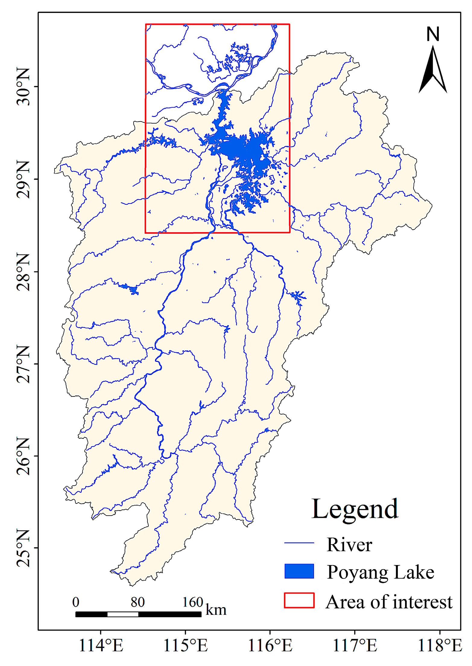
2.1. Study Area

The Poyang Lake (28°22′–29°45′N, 115°47′–116°45′E), is located in the north of the Jiangxi province. It is the largest freshwater lake in China. In the rainy summer season, the area of lake can exceed 4000 km²; in the relatively dry autumn and winter, the lake area will typically shrink by more than 1000 km². The lake is mainly fed by precipitation, and sometimes the Yangtze River flux. Rainy season in the Jiangxi province usually begins in April, and lasts for about three months.

The increase in precipitation causes the water level of the Poyang Lake to rise. The precipitation amount decreases after July. However, the water level of the Yangtze River rises due to the water supply from precipitation and snowmelt in its upper reaches, which feeds the Poyang Lake and makes the water level of this Poyang Lake continue to rise [53] under the continuous influence of human activities and the Yangtze River water diversion and a large amount of sediment deposits, which has an important influence on the area of Poyang Lake.

Figure 1 shows the river networks in the Poyang Lake basin. Since most of the water bodies in the Poyang Lake basin are distributed in the northern region, we have selected an area of interest to compare the water identification effects of different methods. Due to the influence of monsoon precipitation, the spatial coverage of Poyang Lake changes significantly during the wet and dry seasons. Therefore, we select images in summer and winter, respectively, to evaluate the water body recognition effect of the used models.

2.2. Data

The GF-1 satellite was launched in April 2013 and obtained a large amount of data since then. It carries two panchromatic/multi-spectral (P/MS) and four wide-field of view (WFV) cameras. Within the spectral range of the GF-1 WFV sensor (450–890 nm), there are four spectral channels to observe the reflected solar radiation from the earth. It has a spatial resolution of 16 m, a stripe width of 800 km, and consists of four cameras. The temporal resolution is four days. Therefore, it has the characteristics of high frequency revisit time, high spatial resolution and wide coverage, and is an ideal data for large-scale land surface monitoring.

The GF-1 satellite images are provided by the China Resource Satellite Application Center (http://www.cresda.com/CN/). In this study, our model also increases the input channels compared with the conventional neural network, and all the four spectral channels of GF-1 images are used.

2.3. Methods

To produce a water map from high-resolution satellite images, a DenseNet-based water mapping method was proposed. To verify the effectiveness of the proposed method, we compared this method with both methods of water index and classical convolutional neural network.

We select the method of the water index because it is the most widely used and representative method in the field of remote sensing image water extraction. Using the water index, we want to show that the proposed method has better performance than the traditionally used water index in water extraction, and in order to avoid the influence of subjective factors above the threshold selection of water index on the results, we used the Otsu’s threshold segmentation method [54,55] to find the optimal threshold. Due to the limitation of GF-1 spectral bands, we choose the NDWI to extract water.

2.3.1. The Normalized Difference Water Index (NDWI)

The GF-1 images only contain four bands, hence NDWI can only be used to identify the water area. The optimal threshold of NDWI is determined using Otsu’s method. The NDWI is a widely-used method for water identification based on the green band and near-infrared band. Using GF-1 spectral bands, the NDWI is computed as follows:

$$\mathrm{NDWI}=\frac{{\mathrm{b}}_{\mathrm{green}}-{\mathrm{b}}_{\mathrm{near}-\mathrm{infrared}}}{{\mathrm{b}}_{\mathrm{green}}+{\mathrm{b}}_{\mathrm{near}-\mathrm{infrared}}}$$

(1)

where b_green represents the reflectivity of green band, b_{near-infrared} represents the reflectivity of near-infrared band. Ideally, a positive NDWI value indicates the ground is covered with water, rain or snow; a negative NDWI value indicates vegetation coverage; and the ground is covered by rocks or bare soil if the NDWI is equal to 0. The threshold value is always not 0, due to various influences such as vegetation on the water surface. The selection of threshold is a key and difficult problem for accurate water body identification, and we use Otsu’s method to determine it.

This Otsu’s method is a classical algorithm in the image segmentation field which was proposed by the Japanese Nobuyuki Otsu in 1979 [54,55]. It is an adaptive threshold determination method. For a color image, it converts the image into a grayscale image and then distinguishes the target from the background according to the grayscale characteristics. The larger the variance of the gray value between target and the background, the greater the difference between these two parts. So, it calculates the maximum value of the class variance between target and background to find the optimal threshold. Among them, the definition of inter-class variance is as follows:

$${\mathrm{e}}^2\left(\mathrm{T}\right)={\mathrm{P}}_{\mathrm{O}}{(\mathsf{\mu }-{\mathsf{\mu }}_{\mathrm{O}}^{\prime })}^2+{\mathrm{P}}_{\mathrm{b}}{(\mathsf{\mu }-{\mathsf{\mu }}_{\mathrm{b}}^{\prime })}^2$$

(2)

where μ is the grayscale mean of the image, μ_o and μ_b are the means of the target and background, P_o and P_b are the proportion of grayscale of target and background, and T is the threshold. When T is the maximum value of e²(T), it is the optimal threshold.

In this study, as the pixel-wise NDWI values are derived, it is necessary to stretch them to the gray value from 0 to 256, from which Otsu’s threshold is then calculated to segment the water body from the background.

2.3.2. Evolution of Convolutional Neural Network

With the development of technology and the optimization of hardware facilities, many classical networks have emerged after numerous updates of the convolutional neural network. In 2014, researchers developed the new deep convolutional neural network, VGG [30]. They discussed the relationship between the depth and the performance of neural network. VGG [30] successfully constructed the deep layer of 16–19 convolutional neural networks, and it proves that the increase of the network depth affects the performance of the network to some extent. It was once widely used as a backbone feature extraction network for various detection network frameworks [42,56] until the ResNet was proposed.

As a neural network with more than 100 layers, the ResNet’s biggest innovation lies in that it solves the problem of network degradation through the introduction of a residual block. The traditional convolutional network has problems such as information loss during information transmission, and leads to the disappearance of gradient or gradient explosion, which makes the deep network unable to train. ResNet passes the input information directly to the output, thus solving this problem to some extent. It simplifies the difficulty of learning by learning the difference between input and output, instead of all input characteristics. DenseNet was proposed based on ResNet, but with considerable improvement.

As shown in Figure 2, the inputs of each layer of DenseNet are the outputs of all previous layers. The information transmission between different layers of the network is guaranteed to be maximized. Instead of connecting layers over summation such as the ResNet, the DenseNet connects the features through concatenating to achieve feature reuse. Meanwhile, a small growth rate is adopted, and the feature graph of each layer is relatively small; thus, to achieve the same accuracy, the computation required by DenseNet is only about half that of the ResNet. Therefore, this study chooses DenseNet as the backbone to extract features.

For a standard CNN, the output of the layer is the input of the next layer. The ResNet simplifies the training of the deep network by introducing the residual block, of which the output of the layer is the sum of the output of the previous layer and its nonlinear transformation. As for a DenseNet, the input of the l layer is the concatenation of the output characteristic map from 1 to l − 1 layer, and then makes nonlinear changes, that is:

$${\mathrm{x}}_{\mathrm{l}}^{}={\mathrm{K}}_{\mathrm{l}}{\left(\right[\mathrm{x}}_{\mathrm{l}-1}{,\mathrm{x}}_{\mathrm{l}-2}^{},\dots {,\mathrm{x}}_1\left]\right),$$

(3)

here K is made up of batch normalization, activation functions, convolution and dropout. DenseNet’s dense connections increase the utilization of features, make the network easier to train, and has the effect of regularization.

Fully convolutional networks (FCNs) [57,58], as a convolutional neural network, can segment images at pixel scale; therefore, it solves the problem of semantic segmentation. The classic CNN uses the fully connected layers after the convolution layer to obtain the feature vector for classification (fully connected layer + SoftMax output) [59,60,61,62]. Unlike the classic CNN, FCN uses deconvolution to return the reduced feature map to the original size after feature extraction. In this way, while preserving the spatial information of the input, the output with the same size of the input is gradually obtained, so as to achieve the purpose of pixel classification. It can accept input images of any size. Many networks have been proposed for image segmentation after FCN. SegNet [34] was proposed as an encoder–decoder network which uses the first 13 layers of VGG16 as encoders, and the max pooling indices as decoders to improve the segmentation resolution. DeepLab v3+ [39] was proposed in 2018, and it is the latest version of DeepLab series. It uses deep convolutional neural network with atrous convolution in the decoder part. Then the Atrous Spatial Pyramid Pooling (ASPP) is used to introduce multiscale information. Compared with DeepLab v3, v3+ introduces the decoder module, which further integrates the low-level features and high-level features to improve the accuracy of segmentation boundary.

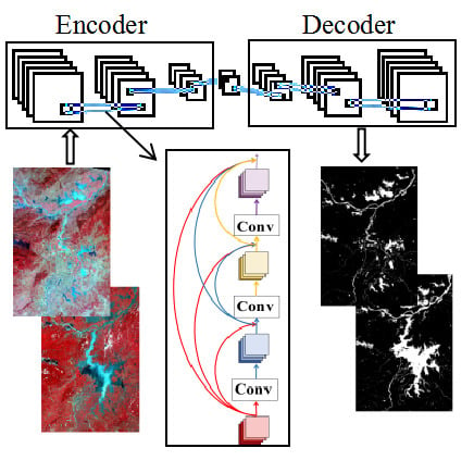
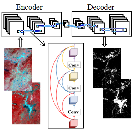
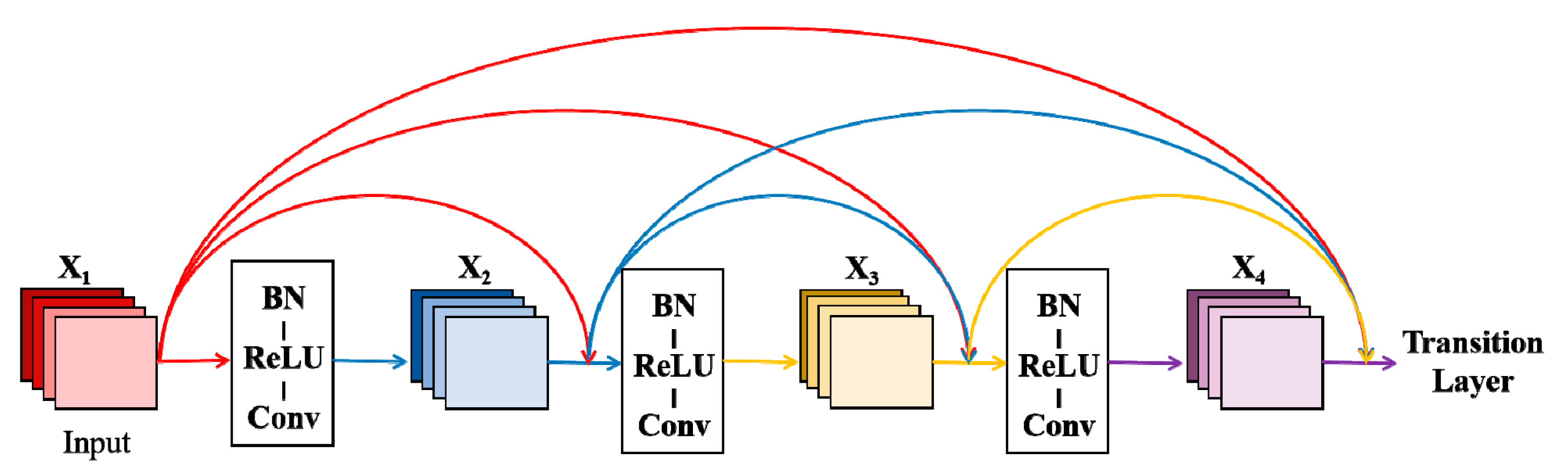
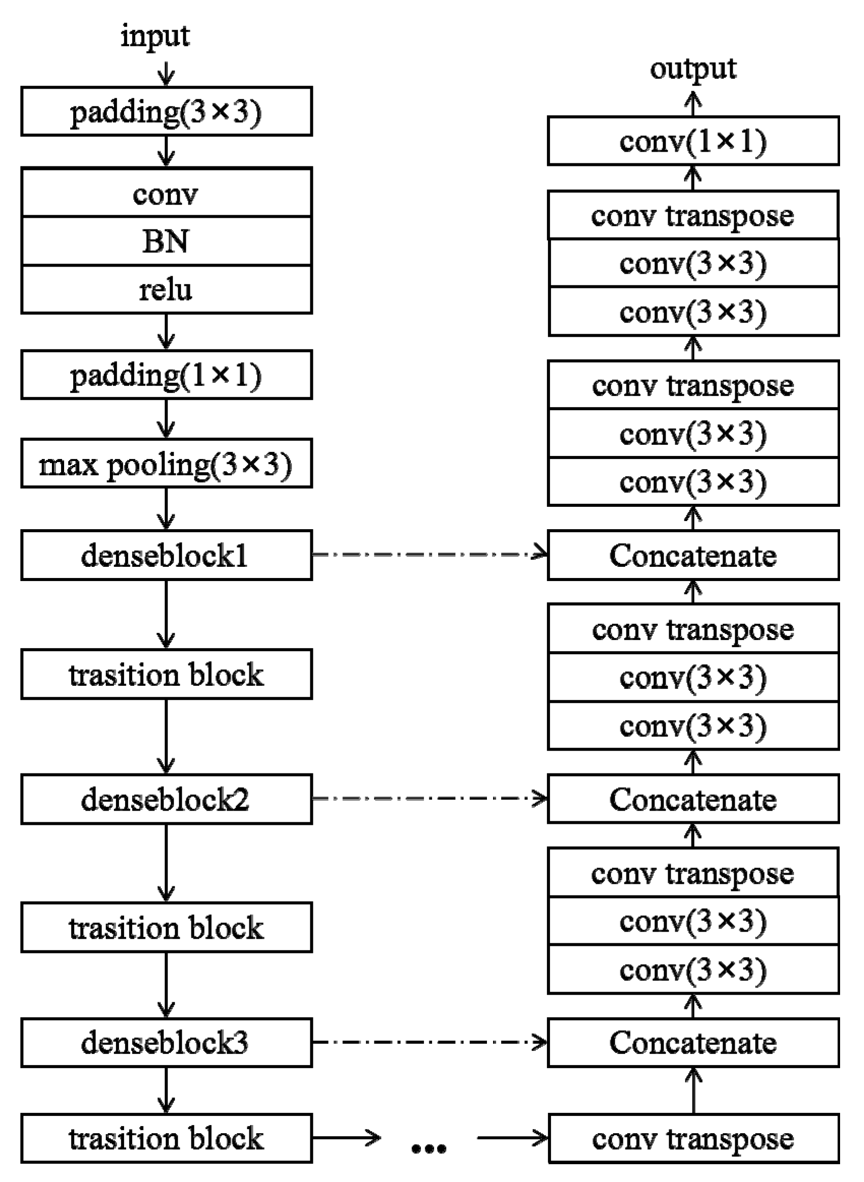
2.3.3. Model-Based on DenseNet

Figure 3 shows the architecture of the network we have proposed for water body identification. Our model is a fully convolutional neural network with the fusion of multiscale features. The model chooses DenseNet as the backbone for feature extraction. The DenseNet we use contains four dense blocks. The transition block makes the connection between each dense block. The transition block consists of a 1 × 1 convolution and a 2 × 2 pooling operation. It can reduce the spatial dimensionality of feature maps.

In our network, in order to recover from the input spatial resolution, the upsampling layer is implemented by the transpose convolution. The feature map of the upsampling is then concatenated to the feature map from the dense block in the down-sampling process. The batch normalization (BN) and the Rectified Linear Unit (ReLU) are performed before the convolution of the image.

Our model can input images of arbitrary size during inference. But for the convenience of training, and to ensure that there is sufficient memory for training, we unified all input images into the size of 224 × 224 pixels. We cut out images of uniform size from GF-1 images, and screened out images containing both water and non-water as effective training data. At the same time, to ensure that the model can directly extract useful features from the original data, we did not do any preprocessing of the input image. We used the Adam optimization algorithm to optimize the weight. Hyperparameters β₁ = 0.9 and β₂ = 0.999 are selected as recommended by the algorithm. We trained our model in stages with the initial learning rate λ = 10⁻⁴, which was reduced by 10 times after 30 epochs. The initial learning rate here is the best result from multiple trials. The growth rate of the network is set as 32, weight decay is 10⁻⁴, and the Nesterov momentum is 0.9, which remain the same as the classic DenseNet.

In order to determine the number of network layers, we experiment with the number of convolutions in each dense block to find the optimal result. The DenseNet proposed by Huang et al. [51] designed three network layers for different tasks, i.e., Densenet121, Densenet169 and Densenet201. In addition to testing the above-mentioned three networks, we also adjust the number of layers to find the most suitable result for this task. We first halve the convolution layers of first three dense blocks of DenseNet121, the fourth block is unchanged, which is DenseNet79.

Then we tried to halve the convolution layers of four blocks and it became DenseNet63. We trained five DenseNets with different network layers to compare which is the best.

In order to make an effective comparison of the results, we use training time as one indicator to determine which network is faster and more convenient. We use the precision (P), recall (R), F1 score (F1) and mean Intersection over Union (mIoU) to quantitatively measure the performance of the network, which are all based on the confusion matrix. The same indicators were used to evaluate the performances of NDWI, VGG, ResNet, SegNet, DeepLab v3+ and DenseNet. As an evaluation index, the confusion matrix evaluates the performance of a classifier, and it is more accurate for the identification results of unbalanced categories. The confusion matrix divides the image identification results into four parts: true positive (TP), true negative (TN), false positive (FP) and false negative (FN). The specific calculation formula of evaluation index is as follows [63]:

$$\mathrm{P}=\frac{\mathrm{TP}}{\mathrm{TP}+\mathrm{FP}}$$

(4)

$$\mathrm{R}=\frac{\mathrm{TP}}{\mathrm{TP}+\mathrm{FN}}$$

(5)

$${\mathrm{F}}_{\mathsf{\alpha }}=\frac{(1+{\mathsf{\alpha }}^2)\mathrm{P}\times \mathrm{R}}{{\mathsf{\alpha }}^2(\mathrm{P}+\mathrm{R})}$$

(6)

$$\mathrm{mIoU}=\frac{\mathrm{TP}}{\mathrm{TP}+\mathrm{FP}+\mathrm{FN}}$$

(7)

where P means the precision, and R means the recall. MIoU is the intersection of two sets of ground truth and predicted results. Precision is the fraction of correctly identified water pixels (TP) among the predicted water pixels (TP + FP) by the model. Recall is the fraction of correctly identified water pixels (TP) among the actual water pixels (TP + FN). Since precision and recall are sometimes contradictory, we further introduce the F1 score to measure the accuracy of a binary model, which simultaneously takes precision and recall into consideration [64]:

$$\mathrm{F}1=\frac{2(\mathrm{P}+\mathrm{R})}{\mathrm{P}+\mathrm{R}}$$

(8)

The comparison results of five networks are shown in

Table 1. Comparison of DenseNets with different layers. The optimal value for each metric is shown in bold. (P refers to Precision; R refers to Recall; F1 refers to F1 score and mIoU refers to mean Intersection over Union).

Network	Time	P	R	F1	mIoU
DenseNet63	15,463 s	0.959	0.900	0.928	0.867
DenseNet79	16,377 s	0.961	0.904	0.931	0.872
DenseNet121	20,611 s	0.957	0.901	0.928	0.866
DenseNet169	24,018 s	0.964	0.896	0.928	0.867
DenseNet201	27,121 s	0.960	0.899	0.929	0.867

. The best results of all indicators are displayed in bold fonts. We can see that with the increase of network layers, the training time also increases; however, the performance does not become better with layer increase. This may be because the input samples of the network are not enough, and the characteristics of the water are easier to identify, so too many layers will not contribute to the results. Among these five networks, DenseNet79 has the best performance in recall, F1 score and mIoU. Its precision is lower than DenseNet169, but the training time is almost two hours less than DenseNet169. Therefore, DenseNet79 is most suitable for the task of water recognition in this study.

To verify the performance of our implementations, VGG, ResNet, SegNet and DeepLab v3+ were selected to make comparisons. VGG and ResNet were selected, respectively, as representatives of the neural network with less than 100 layers, and the neural network with more than 100 layers. SegNet and DeepLab v3+ were selected as representatives of two segmentation network structures: encoder–decoder structure and Atrous convolution. Also, due to the limitation of computation resources and the number of training datasets, it is not necessary to use powerful and complicated networks as our exception, since, as the backbone of DeepLab v3+, we chose MobileNet [65] as the backbone, which has much less parameter, and can achieve good results on our task in shorter time.

3. Results

To see if the DenseNet is more suitable and efficient than the other methods, we first compare the result of the proposed network with the ground truth to evaluate its effectiveness in identifying the water bodies. Then we compare with the results derived from the NDWI index and four other deep neural networks of VGG, ResNet, SegNet and DeepLab v3+. Finally, we chose the best model and made a simple analysis of the changes in water areas in Poyang Lake area in winter and summer from 2014 to 2018.

3.1. The Image Preprocessing

The dataset contains GF-1 images from the middle and lower reaches of the Yangtze River basin in different periods. The corresponding labels were binary classifications of the water–nonwater area by expert visual interpretation. To improve the efficiency of the model training, we clipped the input data to 224 × 224 pixels. We have deliberately selected some labels with both land and water bodies as training samples. Finally, we have selected 5558 water bodies samples. Of these, 4446 images were used as training sets, while the remaining 1112 images were used as test sets. This data is only used for model training and quantitative evaluation. Since the samples are cut into small pieces, and the selection of training set and test set are random, the recognition efficiency of the model on a large range of images cannot be seen from the existing data. To qualitatively evaluate the performance of different models in different ground object types, we also applied the model to other GF-1 images in different periods.

3.2. Water Identification Result of DenseNet

Figure 4 is the recognition result of 12 remote sensing images selected from the validation dataset, the corresponding ground truths, and the DenseNet result. The sizes of images are all 224 × 224. These 12 images contain water bodies of various shapes and colors, from which the recognition effectiveness of this model on different water bodies can be understood.

It can be seen from Figure 4 that the recognition result of DenseNet is consistent with the ground truth. Although this model failed to identify some small water bodies, the error areas are generally very small, and such small errors have little influence on the overall distribution of water bodies, which can be ignored. In addition, the network can accurately identify the water bodies in different forms and regions, and accurately separate small rivers in the towns, and even small barriers such as bridges in the water can be correctly separated. The boundaries between water and land were identified, partly because of the fine resolution of the GF-1 images, and partly because of the efficiency of the proposed DenseNet model.

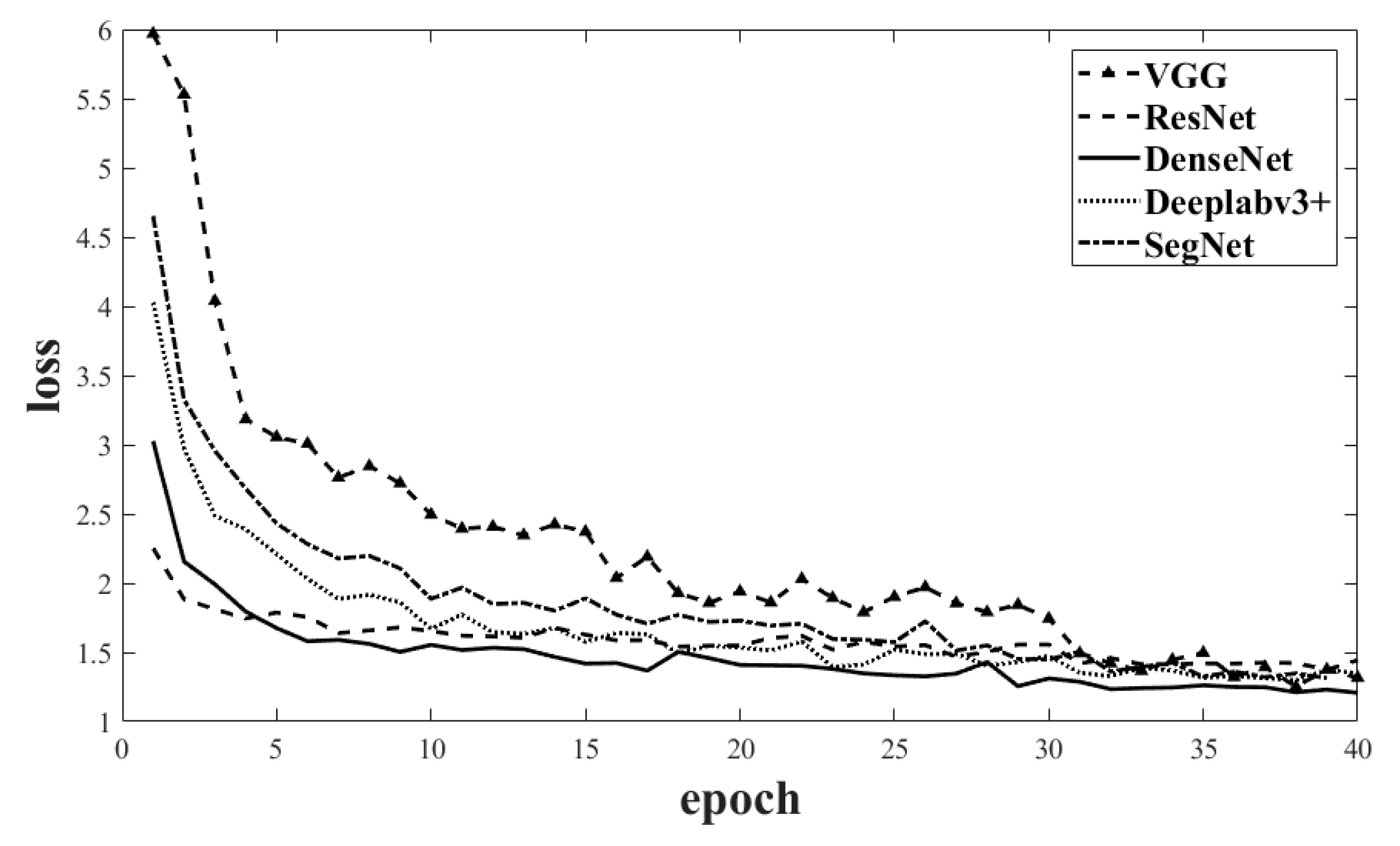
3.3. Working Efficiency of DenseNet, ResNet, VGG, SegNet and DeepLab v3+ Models

Figure 5 shows the training losses of DenseNet, ResNet, VGG, SegNet and DeepLab v3+. In the convolutional neural networks, the loss function is used to calculate the difference between the output of the model and the ground truth, so as to better optimize the model. The smaller the loss is, the better the robustness of the model is. In Figure 5, one epoch represents 1000 iterations. For the initial epochs, the loss value of VGG is by far the highest, which is two or three times higher than those of ResNet and DenseNet; and it remains the highest until 30 epochs. The initial loss value of SegNet is close to VGG, followed by DeepLab v3+. The DenseNet has a higher initial loss value than the ResNet, but then it declines faster than the ResNet and continues to be lower than the ResNet after five epochs. The loss of DenseNet maintains the lowest after five epochs, indicating the fastest convergence speed compared to the other four models.

Table 2. Training time of the DenseNet, ResNet, VGG, SegNet and DeepLab v3+ models.

Network	Time
DenseNet	16,377 s
ResNet	19,436 s
VGG	21,471 s
SegNet	19,021 s
DeepLab v3+	11,924 s

shows the training time of the five networks. Among them, the VGG has the longest training time. The DeepLab v3+’s training time is the shortest, and DenseNet is next to it. The DenseNet saves about 80 min compared to the VGG model, about 50 min compared to the ResNet model, and 40 min compared to the SegNet model.

But it takes more than 70 min compared to DeepLab v3+. This indicates that under the same training environment, the DeepLab v3+ requires the least training time; it is easier to train and use the lowest resource consumption capacity. The reason why we did not compare the time consumption of NDWI with these networks is that the NDWI method does not need a lot of time to process, and the required time can be ignored.

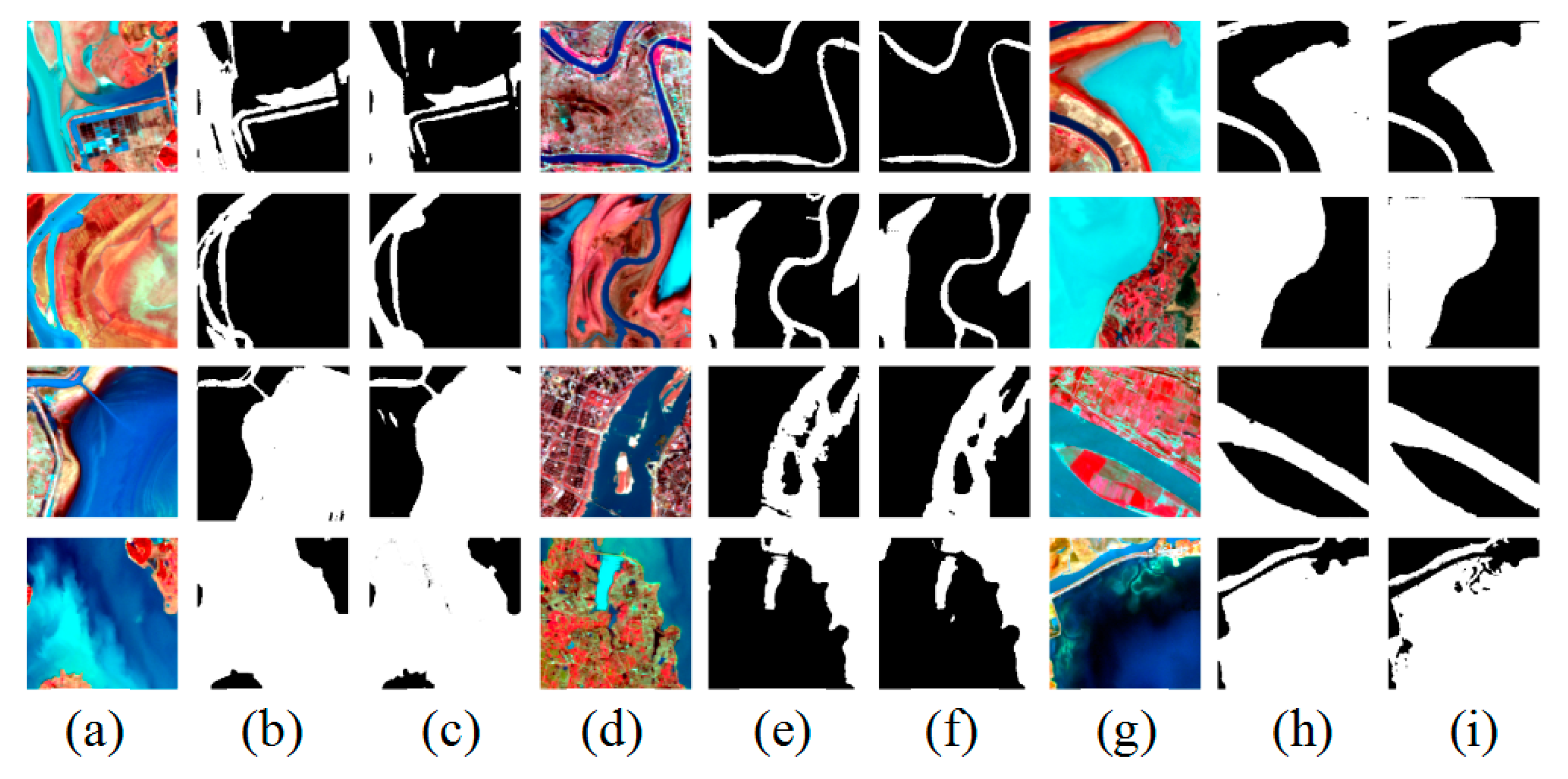
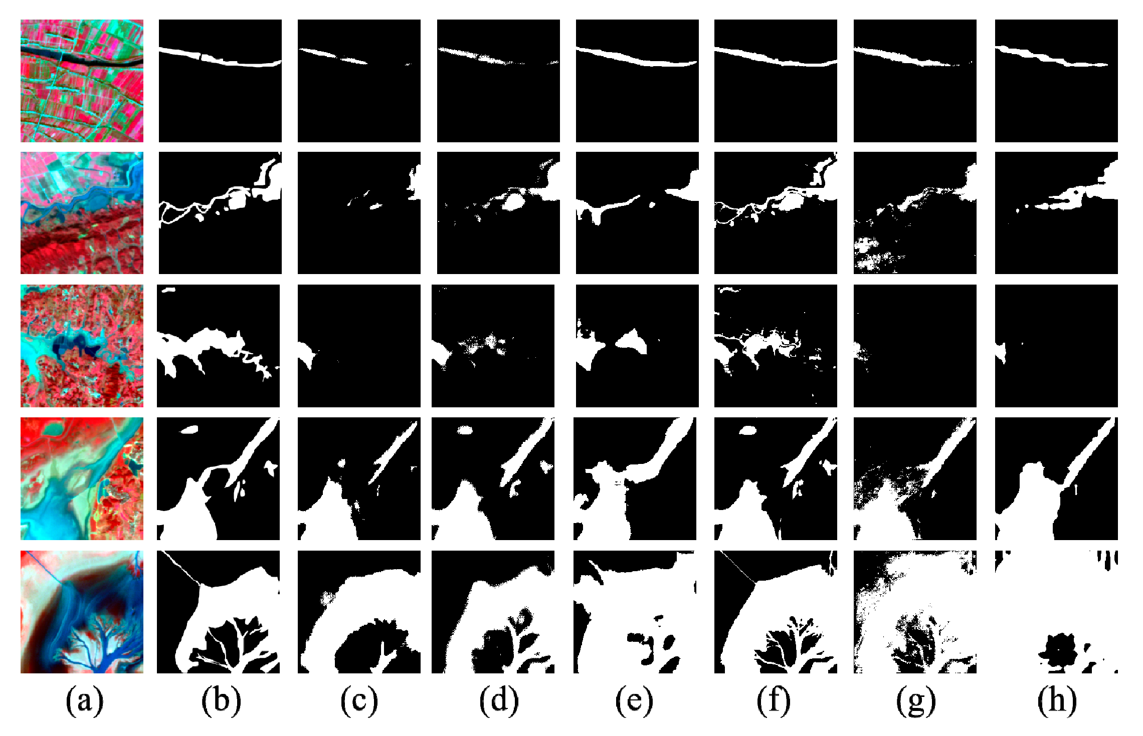
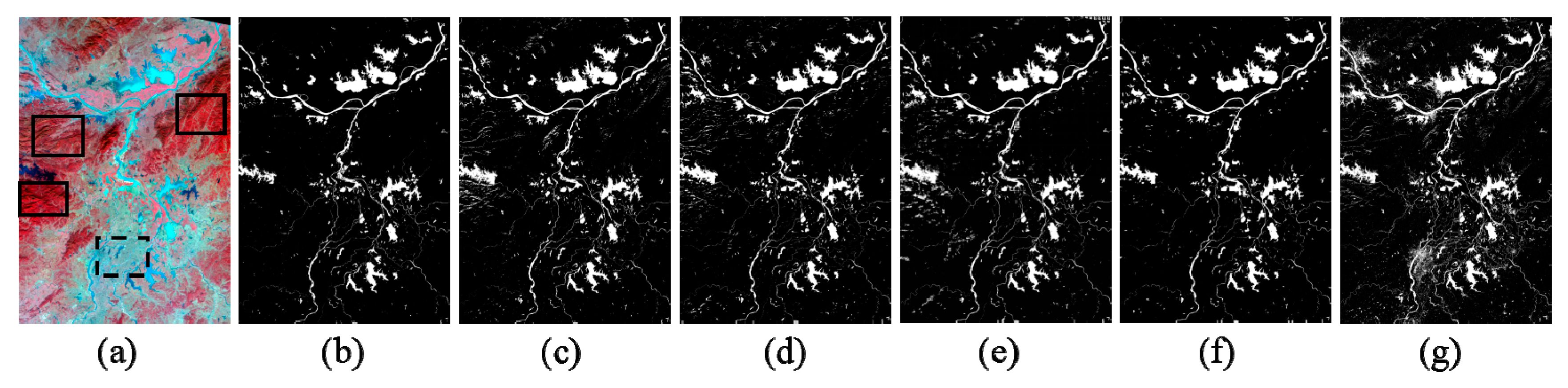
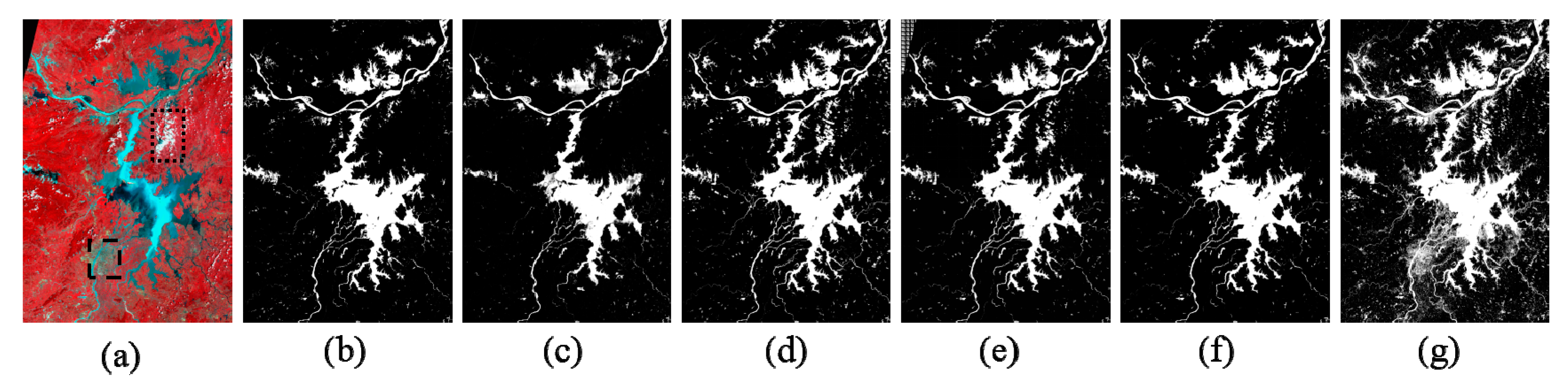
3.4. Comparison of Identification Results

The derived P, R, F1 score and mIoU of the VGG, the ResNet, the DenseNet, the SegNet, the DeepLab v3+ and the NDWI models are shown in

Table 3. The derived P, R, F1score and mIoU of the VGG, ResNet, DenseNet, SegNet, DeepLab v3+ and NDWI models with 95% confidence interval. The optimal value for each metric is shown in bold.

	DenseNet	ResNet	VGG	SegNet	DeepLab v3+	NDWI
P	0.961 ± 0.011	0.936 ± 0.014	0.914 ± 0.016	0.911 ± 0.017	0.922 ± 0.016	0.702 ± 0.027
R	0.904 ± 0.017	0.902 ± 0.017	0.915 ± 0.016	0.934 ± 0.015	0.917 ± 0.016	0.983 ± 0.007
F1	0.931 ± 0.015	0.919 ± 0.016	0.914 ± 0.016	0.922 ± 0.016	0.919 ± 0.016	0.819 ± 0.023
mIoU	0.872 ± 0.020	0.850 ± 0.021	0.842 ± 0.021	0.856 ± 0.021	0.850 ± 0.021	0.767 ± 0.025

. All values in the table were calculated by the prediction results of 1112 images in the test set, and their corresponding ground truth. Given the limited number of samples, we reported the 95% confidence interval of the metrics to see if the result is statistically significant. The best result of each indicator is in bold. We can see from the results that all neural networks’ results are much better than the NDWI index. For each network model, the DenseNet result, with a narrower interval, appears more stable than the other methods.

Among six models, the DenseNet appears to have the highest precision of 0.961, meaning that 96.1% of the water bodies are correctly predicted among the predicted water bodies by the model. The precisions of ResNet, VGG, SegNet and DeepLab v3+ are 0.936, 0.914, 0.911 and 0.922, respectively. Such a rank of this precision is as expected, considering the pathway of theoretical improvements of these deep neural network models. However, the NDWI model based on the spectral bands appears to have a rather reduced prediction precision, which is only 0.702, although an adaptive threshold from the Otsu method is employed. Hence, the DenseNet appears to perform the best among the three deep neural networks regarding prediction precision; particularly, such a neural network, at least in this case, is by far the better than normally used NDWI method for water body identification in the remote sensing community.

Among the three deep neural networks, SegNet shows the highest recall value of 0.934. The ResNet shows the lowest recall, which is 0.902. The DenseNet is only 0.02 higher than ResNet. VGG and DeepLab v3+ have a recall of 0.915 and 0.917, respectively. The NDWI model shows the highest recall value of 0.983 among all the six methods, indicating it has successfully identified most of the water body samples in the training dataset. However, its precision value is the lowest, indicating that there are still serious ill predictions from this method. As can be seen, the matrices of recall and precision have given contrary indications of the model performances. To make a comprehensive evaluation of these two indicators, we investigate the F1 score considering both the precision and the recall values. We also use mIoU to evaluate the accuracy of model segmentation results. A higher F1 score and mIoU indicates a better performance. The F1 scores of the DenseNet, ResNet, VGG, SegNet and DeepLab v3+ models are 0.931, 0.919, 0.914, 0.922 and 0.919, respectively, and the mIoUs of them are 0.872, 0.850, 0.842, 0.856 and 0.850, respectively. We can see from the results that the performance of DenseNet is better than ResNet, VGG, SegNet and DeepLab v3+. This may be due to the dense connection, which increases the utilization efficiency of the features. As for the result of DeepLab v3+, the training efficiency is much better than DenseNet. This is because the backbone of DeepLab v3+ we chose is MobileNet, which is a lightweight network using the depth-wise separable convolution to reduce the number of parameters and the amount of calculation. The F1 score and the mIoU of the NDWI index are as low as 0.819 and 0.767, showing that all the deep neural networks have much better performance than the traditional NDWI method from a comprehensive viewpoint.

The recalls of DenseNet and ResNet are not very good in these models, meaning that these networks are not good at capturing all the water areas. Figure 6 shows some examples of this disadvantage. The third column is the result of DenseNet, and the fourth column is the result of ResNet; this figure shows that the water area which DenseNet recognized is the smallest in all six models, and it distributes in small rivers and intertidal zones. Column (h) is the result of NDWI. NDWI recognized the biggest water area, which is consistent with its highest recall value. However, with the increase of identified water area, the probability of recognition error is also increasing, meaning that the precision is more likely to drop with it. To increase the recall value of DenseNet, it may cost a sharp drop of precision. It has good results of F1 score and mIoU, meaning that the overall performance of this network is very good. Therefore, we decided not to further optimize the recall of DenseNet.

In order to further understand the performance of each method in different regions, we selected two GF-1 images of the Poyang Lake during the wet and the dry seasons, respectively, to evaluate the performance of different models, i.e., 29 July and 31 December 2016. Figure 7 shows the results from the image on 31 December 2016, when the Poyang Lake basin was dry with a complex distribution of water area.

In the false-color image, the blue area is mostly water body, and the red area is mostly vegetated. The other colored areas include bare land, buildings and other nonwater areas. The mountain area is depicted with a solid line frame, while the urban area is marked with a dashed line frame. In the prediction results of ResNet, many patches in the corresponding region of the mountains are predicted to be water bodies, which proves that the ResNet model is prone to confuse mountain shadows with water. In the same regions, the VGG and SegNet models have also falsely identified some mountain shadow areas as water bodies. DeepLab v3+ has not confused the mountain shadow with a water body, but the boundary of water area it extracted was not as concise as the other methods. The main water body was correctly identified by the NDWI models, which are however much larger than the actual water bodies, and the NDWI model has also identified too many fine patches. The NDWI result also had false detection of the mountain shadows, which is larger than those from the ResNet model, but smaller than those from the VGG model. Other than the mountain shadow, the biggest problem with the NDWI result is that it falsely identified some bare land and urban construction areas as water bodies. The DenseNet model has successfully identified the small rivers and lakes from the GF-1 image, and the mountain shadows and water bodies are successfully separated. In general, these five deep neural networks have consistently identified the large water bodies in winter, although the ResNet and the VGG models show a false identification of mountain shadows. These neural networks have performed much better than the traditionally used NDWI water body index.

Figure 8 shows the identified water bodies from the GF-1 image on 29 July 2016. In the false-color image, the white area in the dotted line indicates the cloud, and the dashed line depicts the urban area. In summer, the Poyang Lake is in a season with abundant water, and its water area reaches its peak within a year. It is found that the VGG, SegNet and DeepLab v3+ models have falsely identified the cloud as water bodies, and the DenseNet also has a small amount of false identification. We can see that the NDWI index can better identify the bulk of the water body, but there is much noise in the boundary areas; besides, it has falsely identified the urban buildings, bare ground and most clouds as water bodies. It is the ResNet model that completely distinguishes between the cloud and the water bodies, which however has some false identification of some water bodies. As for the DenseNet result, it shows a relatively accurate identification of water bodies with clear boundary separation for the transitional areas between land and water. The DenseNet method partially falsely identified cloud as water bodies, but it has filtered out most of it compared to the NDWI result.

Therefore, for the image of 29 July 2016, these five deep networks have their advantages and disadvantages for the water body identification, but overall show better performances than the NDWI method.

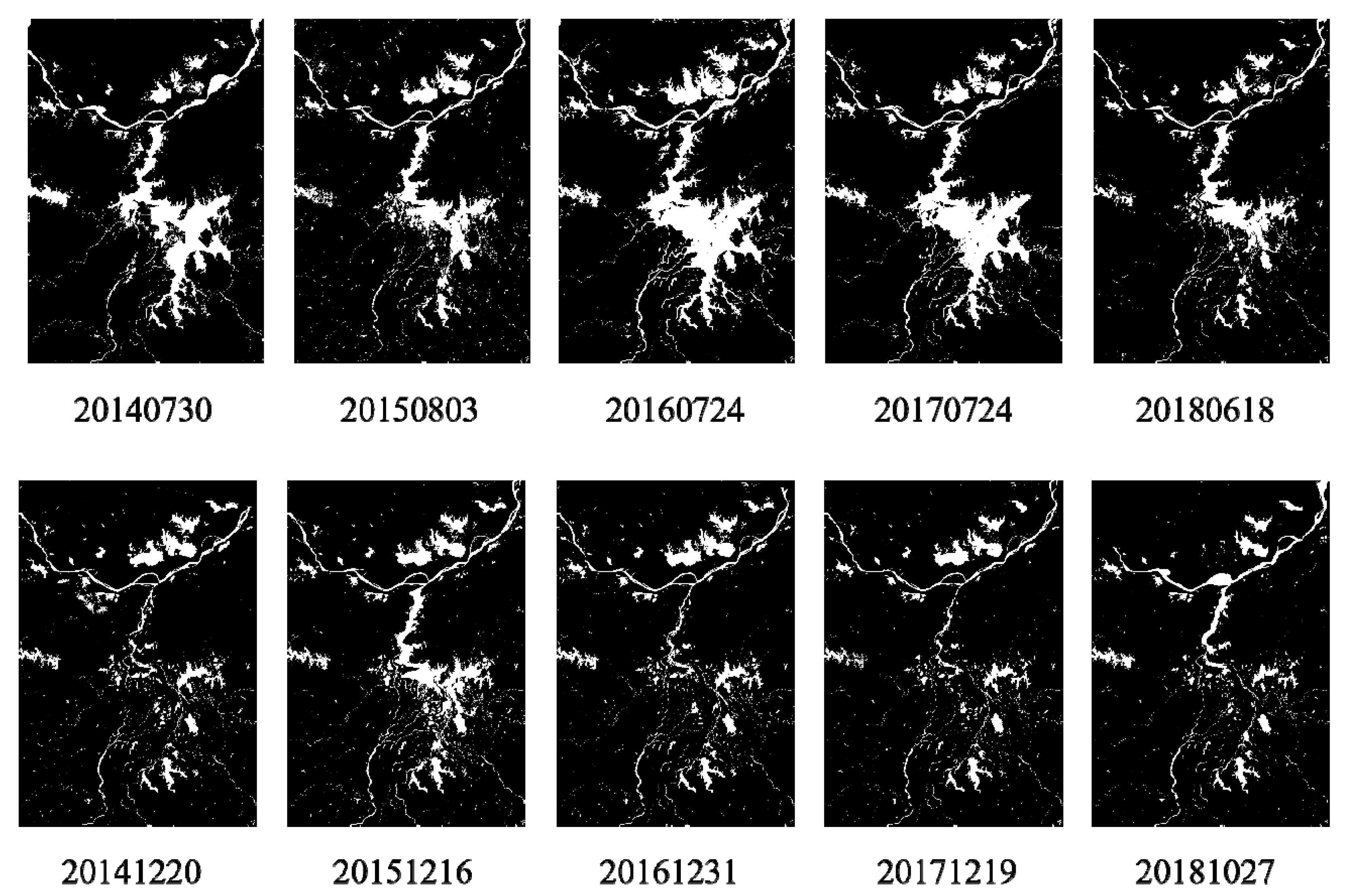
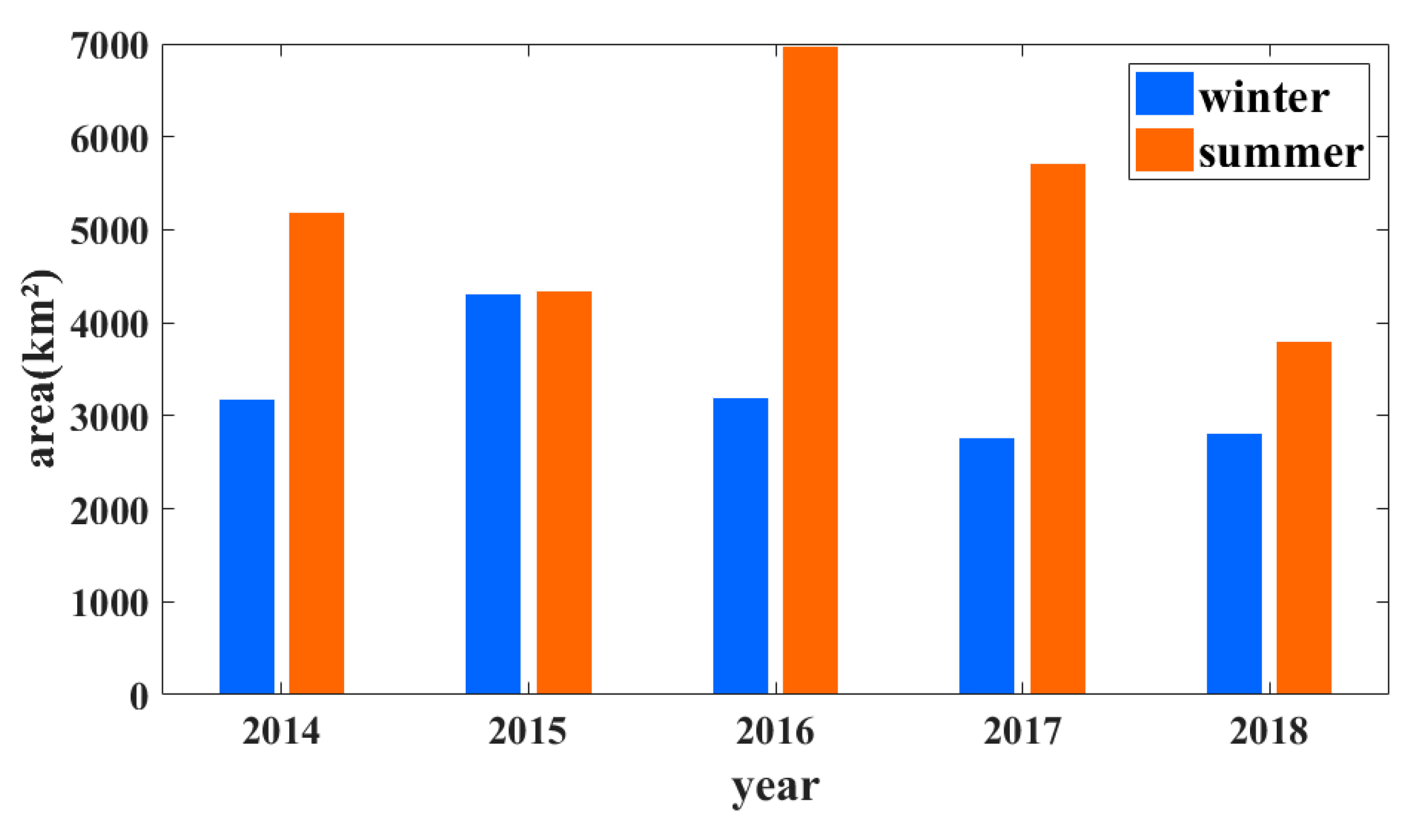
3.5. Interannual Variations of the Water Areas

It can be concluded from the above results that the DenseNet model we proposed has higher accuracy, and can be used for water body identification. Therefore, we have used this model to understand the interannual changes of water areas of Poyang Lake. Since GF-1 was successfully launched in late 2013, we could only study the water area changes from 2014 to 2018. The water areas of Poyang Lake change significantly among seasons, and there is a huge difference between the wet and the dry seasons. The first row of Figure 9 shows the spatial distribution of Poyang Lake in summer from 2014 to 2018. The water area in 2016 was the largest, when there was a flooding disaster event in the Yangtze River basin, and the area in 2018 was the smallest when there was a summer drought due to the reduced precipitation. The second row shows the lake areas in winter. The water areas of Poyang Lake decrease sharply in winter, and the main lake body shrinks to only tributaries and smaller lakes. The disappearance of Poyang Lake is mainly concentrated in the central and southern parts of the lake, leaving only a small part of the water body in the north and northeast. This is principally due to the climatic conditions but is also partly related to the topography, the Yangtze River runoff and the three gorges dam [66,67].

Figure 10 shows the interannual variations of water areas of the Poyang Lake in summer and winter respectively, which were derived from GF-1 images from 2014 to 2018 based on the DenseNet model. The water areas in summer season are generally much larger than those in winter; this is not surprising, because summer is the rainy season in the Poyang Lake basin. The difference in the lake areas in winter and summer is about 2000 km² on average. The water area in 2014 summer is about 5200 km² and that in winter is about 3200 km². In 2015, the water areas in summer and winter are equivalent, amounting to about 4300 km²; this is because of the increased winter precipitation and reduced summer precipitation contrasting to the normal years. In 2016, the water area in winter is about 3250 km² and that doubles in summer, reaching 7000 km² due to a severe flooding. It appears clearly that the water areas in summer are decreasing rapidly from 2016 on; however, those in winter show relatively small changes.

4. Discussion

It can be seen from the above results that the performance of a traditionally used water index method is not satisfying, especially in urban areas. This indicates the common problems of water index which are, at least partly, based on thresholds: the thresholds change largely with time and space; the determination of threshold is highly subjective and contains a lot of background information [20,52]. The biggest advantage of NDWI lies in that it is simple and can generate a water map in a very short time. The proposed DenseNet-based water identification method can extract water bodies from the GF-1 images with high accuracy, but it needs hours of training time. However, considering the improvement it has made in recognition accuracy, and once the network is trained, the time to use this network is comparable to NDWI.

So, this network is still a better tool compared to the water index method. Meanwhile, the comparison of the proposed method with other four neural networks shows that it is a more powerful tool for water body recognition.

There are more and more studies using the deep convolution neural network to classify remote sensing images [68]. Our results have approved that, for big remote sensing data like GF-1 images with high spatial and temporal resolutions, the deep learning method can be used to extract water bodies with accurate results efficiently. It can be seen from water area changes in the recent years that the derived water areas from the deep learning method can well reflect the local drought or flooding conditions. Therefore, using the proposed method, the changes of water bodies, such as river and lakes, and wetland as well, can be timely and effectively monitored [69].

The algorithm proposed in this study shows a certain deviation in distinguishing water bodies and clouds, which can be further improved by modifying the model structure and parameters. Also, the cloud area can be removed using image preprocessing to avoid such misjudgment. In this study, we did not preprocess to remove the cloud, such that the original information of the input images are kept. In addition, we use the cloud as one of the indicators to evaluate the effect of water recognition algorithm. When a flooding event occurs, the cloud is always a barrier for water body monitoring with optical remote sensing image. In such a case, the identification results can be improved by removing clouds first or adding samples containing clouds. For cloud removal, it is a solution to integrate optical with microwave remote sensing images. The deficiency of optical remote sensing can be made up by combining with the advantage of microwave remote sensing to penetrate clouds and fog [70,71].

5. Conclusions

This study presents a new multidimensional, densely connected, convolutional network for water identification from high spatial resolution multispectral remote sensing images. It uses DenseNet as the feature extraction network to carry out image downs-sampling, then uses trans-convolution for image upsampling. On this basis, multiscale fusion is added to fuse features of different scales in the down-sampling process into the upsampling process. Compared with the traditionally used water index method, the deep convolutional neural network does not need to find the index threshold, leading to reduced errors, and thus higher accuracy. Meantime, comparing the proposed DenseNet with other networks of ResNet, VGG, SegNet and DeepLab v3+, this DenseNet method requires less training time and has the fastest convergence speed besides DeepLab v3+. The overall performance of DenseNet is still much better. We also added a 95% confidence interval to the evaluation results to reduce the uncertainty caused by the limited samples. The results from the GF-1 images show that, even though DenseNet cannot identify all of the water areas, but it can identify water with great precision, and has much better performance in identifying the boundary between land and water, and can better distinguish the mountain shadows, towns and bare land. Its performance is also better in terms of distinguishing the cloud. Furthermore, the proposed deep learning approach can be easily generalized to an automatic program.

References

1. Tri, A.; Dong, L.; In, Y.; In, Y.; Jae, L. Identification of Water Bodies in a Landsat 8 OLI Image Using a J48 Decision Tree. Sensors 2016, 16, 1075. [Google Scholar]
2. Shevyrnogov, A.P.; Kartushinsky, A.V.; Vysotskaya, G.S. Application of Satellite Data for Investigation of Dynamic Processes in Inland Water Bodies: Lake Shira (Khakasia, Siberia), A Case Study. Aquat. Ecol. 2002, 36, 153–164. [Google Scholar] [CrossRef]
3. Famiglietti, J.S.; Rodell, M. Water in the Balance. Science 2013, 340, 1300–1301. [Google Scholar] [CrossRef] [PubMed]
4. Feng, L.; Hu, C.; Han, X.; Chen, X. Long-Term Distribution Patterns of Chlorophyll-a Concentration in China’s Largest Freshwater Lake: MERIS Full-Resolution Observations with a Practical Approach. Remote Sens. 2015, 7, 275–299. [Google Scholar] [CrossRef] [Green Version]
5. Ye, Q.; Zhu, L.; Zheng, H.; Naruse, R.; Zhang, X.; Kang, S. Glacier and lake variations in the Yamzhog Yumco basin, southern Tibetan Plateau, from 1980 to 2000 using remote-sensing and GIS technologies. J. Glaciol. 2007, 53, 183. [Google Scholar] [CrossRef] [Green Version]
6. Zhang, F.; Zhu, X.; Liu, D. Blending MODIS and Landsat images for urban flood mapping. Int. J. Remote Sens. 2014, 35, 3237–3253. [Google Scholar] [CrossRef]
7. Barton, I.J.; Bathols, J.M. Monitoring flood with AVHRR. Remote Sens. Environ. 1989, 30, 89–94. [Google Scholar] [CrossRef]
8. Sheng, Y.; Gong, P.; Xiao, Q. Quantitative dynamic flood monitoring with NOAA AVHRR. Int. J. Remote Sens. 2001, 22, 1709–1724. [Google Scholar] [CrossRef]
9. Davranche, A.; Lefebvre, G.; Poulin, B. Wetland monitoring using classification trees and SPOT-5 seasonal time series. Remote Sens. Environ. 2012, 114, 552–562. [Google Scholar] [CrossRef] [Green Version]
10. Kelly, M.; Tuxen, K.A.; Stralberg, D. Mapping changes to vegetation pattern in a restoring wetland: Finding pattern metrics that are consistent across spatial scale and time. Ecol. Indic. 2011, 11, 263–273. [Google Scholar] [CrossRef]
11. Zhao, G.; Xu, Z.; Pang, B.; Tu, T.; Xu, L.; Du, L. An enhanced inundation method for urban flood hazard mapping at the large catchment scale. J. Hydrol. 2019, 571, 873–882. [Google Scholar] [CrossRef]
12. Jamshed, A.; Rana, I.A.; Mirza, U.M.; Birkmann, J. Assessing relationship between vulnerability and capacity: An empirical study on rural flooding in Pakistan. Int. J. Disaster Risk Reduct. 2019, 36, 101109. [Google Scholar] [CrossRef]
13. Minaee, S.; Wang, Y. An ADMM Approach to Masked Signal Decomposition Using Subspace Representation. IEEE Trans. Image Process. 2019, 28, 3192–3204. [Google Scholar] [CrossRef] [PubMed] [Green Version]
14. Frazier, P.S.; Page, K.J. Water body detection and delineation with Landsat TM data. Photogramm. Eng. Remote Sens. 2000, 66, 1461–1467. [Google Scholar]
15. Berthon, J.F.; Zibordi, G. Optically black waters in the northern Baltic Sea. Geophys. Res. Lett. 2010, 37, 232–256. [Google Scholar] [CrossRef]
16. Karpatne, A.; Khandelwal, A.; Chen, X.; Mithal, V.; Faghmous, J.; Kumar, V. Global Monitoring of Inland Water Dynamics: State-of-the-Art, Challenges, and Opportunities; Lässig, J., Kersting, K., Morik, K., Eds.; Computational Sustainability, Springer International Publishing: Cham, Switzerland, 2016; pp. 121–147. [Google Scholar]
17. Bischof, H.; Schneider, W.; Pinz, A.J. Multispectral classification of Landsat-images using neural networks. IEEE Trans. Geosci. Remote Sens. 1992, 30, 482–490. [Google Scholar] [CrossRef]
18. Hughes, M.J.; Hayes, D.J. Automated detection of cloud and cloud shadow in single-date Landsat imagery using neural networks and spatial post-processing. Remote Sens. 2014, 6, 4907–4926. [Google Scholar] [CrossRef] [Green Version]
19. Mcfeeters, S.K. The use of the Normalized Difference Water Index (NDWI) in the delineation of open water features. Int. J. Remote Sens. 1996, 17, 1425–1432. [Google Scholar] [CrossRef]
20. Xu, H. Modification of normalised difference water index (NDWI) to enhance open water features in remotely sensed imagery. Int. J. Remote Sens. 2006, 27, 3025–3033. [Google Scholar] [CrossRef]
21. Feyisa, G.L.; Meilby, H.; Fensholt, R.; Proud, S.R. Automated water extraction index: A new technique for surface water mapping using Landsat imagery. Remote Sens. Environ. 2014, 40, 23–35. [Google Scholar] [CrossRef]
22. Zhu, C.; Luo, J.; Shen, Z.; Li, J. River Linear Water Adaptive Auto-extraction on Remote Sensing Image Aided by DEM. Acta Geodaetica et Cartographica Sinica 2013, 42, 277–283. [Google Scholar]
23. Tesfa, T.K.; Tarboton, D.G.; Watson, D.W.; Schreuders, K.A.T.; Baker, M.E.; Wallace, R.M. Extraction of hydrological proximity measures from DEMs using parallel processing. Environ. Modell. Softw. 2011, 26, 1696–1709. [Google Scholar] [CrossRef]
24. Turcotte, R.; Fortin, J.P.; Rousseau, A.N.; Massicotte, S.; Villeneuve, J.P. Determination of the drainage structure of a watershed using a digital elevation model and a digital river and lake network. J. Hydrol. 2001, 240, 225–242. [Google Scholar] [CrossRef]
25. Chen, C.; Fu, J.; Sui, X.; Lu, X.; Tan, A. Construction and application of knowledge decision tree after a disaster for water body information extraction from remote sensing images. J. Remote Sens. 2018, 2, 792–801. [Google Scholar]
26. Xia, X.; Wei, Y.; Xu, N.; Yuan, Z.; Wang, P. Decision tree model of extracting blue-green algal blooms information based on Landsat TM/ETM + imagery in Lake Taihu. J. Lake Sci. 2014, 26, 907–915. [Google Scholar]
27. Liu, W.; Wang, Z.; Liu, X.; Zeng, N.; Liu, Y.; Alsaadi, F.E. A survey of deep neural network architectures and their applications. Neurocomputing 2017, 234, 11–26. [Google Scholar] [CrossRef]
28. Krizhevsky, A.; Sutskever, I.; Hinton, G.E. ImageNet Classification with Deep Convolutional Neural Networks. In Proceedings of the Neural Information Processing Systems, Lake Tahoe, NV, USA, 3–6 December 2012; pp. 1097–1105. [Google Scholar]
29. Szegedy, C.; Liu, W.; Jia, Y.; Sermanet, P.; Reed, S.; Anguelov, D.; Erhan, D.; Vanhoucke, V.; Rabinovich, A. Going Deeper with Convolutions. In Proceedings of the IEEE Conference on Computer Vision and Pattern Recognition, Boston, MA, USA, 7–12 June 2015; pp. 1–9. [Google Scholar]
30. Simonyan, K.; Zisserman, A. Very Deep Convolutional Networks for Large-Scale Image Recognition. Available online: https://www.arxiv-vanity.com/papers/1409.1556/ (accessed on 18 December 2019).
31. He, K.; Zhang, X.; Ren, S.; Sun, J. Deep Residual Learning for Image Recognition. In Proceedings of the IEEE Conference on Computer Vision and Pattern Recognition, Las Vegas, NV, USA, 26–30 June 2016; pp. 770–778. [Google Scholar]
32. Santoro, A.; Faulkner, R.; Raposo, D.; Rae, J.; Chrzanowski, M.; Weber, T.; Wierstra, D.; Vinyals, O.; Pascanu, R.; Lillicrap, T. Relational Recurrent Neural Networks. Available online: https://arxiv.org/abs/1806.01822 (accessed on 18 December 2019).
33. Ronneberger, O.; Fisher, P.; Brox, T. U-Net: Convolutional Networks for Biomedical Image Segmentation. In Proceedings of the Medical Image Computing and Computer Assisted Intervention, Munich, Germany, 5–9 October 2015; pp. 234–241. [Google Scholar]
34. Badrinarayanan, V.; Kendall, A.; Clipolla, R. A Deep Convolutional Encoder-Decoder Architecture for Image Segmentation. IEEE Trans. Pattern Anal. Mach. Intell. 2017, 39, 2481–2495. [Google Scholar] [CrossRef] [PubMed]
35. Lin, G.; Milan, A.; Shen, C.; Reid, I. Refine Net: Multi-Path Refinement Networks for High-Resolution Semantic Segmentation. Available online: https://arxiv.org/abs/1611.06612 (accessed on 18 December 2019).
36. Chen, L.C.; Papandreou, G.; Kokkinos, I.; Murphy, K.; Yuille, A.L. Semantic Image Segmentation with Deep Convolutional Nets and Fully Connected CRFs. Available online: https://arxiv.org/abs/1412.7062 (accessed on 10 February 2020).
37. Chen, L.C.; Papandreou, G.; Kokkinos, I.; Murphy, K.; Yuille, A.L. DeepLab: Semantic Image Segmentation with Deep Convolutional Nets, Atrous Concolution, and Fully Connected CRFs. Available online: https://arxiv.org/abs/1606.00915 (accessed on 10 February 2020).
38. Chen, L.C.; Papandreou, G.; Schroff, F.; Papandreou, G. Rethinking Atrous Convolution for Semantic Image Segmentation. Available online: https://arxiv.org/abs/1706.05587 (accessed on 10 February 2020).
39. Chen, L.C.; Zhu, Y.; Papandreou, G.; Schroff, F.; Papandreou, G. Encoder-Decoder with Atrous Separable Convolution for Semantic Image Segmentation. In Proceedings of the European Conference on Computer Vision, Munich, Germany, 8–14 September 2018; pp. 833–851. [Google Scholar]
40. Zhao, H.; Shi, J.; Qi, X.; Wang, X.; Jia, J. Pyramid Scene Parsing Network. In Proceedings of the IEEE Conference on Computer Vision and Pattern Recognition, Honolulu, HI, USA, 21–26 July 2017; pp. 6230–6239. [Google Scholar]
41. Girshick, R.; Donahue, J.; Darrel, T.; Malik, J. Rich feature hierarchies for accurate object detection and semantic segmentation. Available online: https://arxiv.org/abs/1311.2524 (accessed on 10 February 2020).
42. Girshick, R. Fast R-CNN. In Proceedings of the International Conference on Computer Vision, Santiago, MN, USA, 13–16 December 2015; pp. 1440–1448. [Google Scholar]
43. Ren, S.; He, K.; Girshick, R.; Sun, J. Faster R-CNN: Towards Real-Time Object Detection with Region Proposal Networks. In Advances in Neural Information Processing Systems 28; Cortes, C., Lawrence, N.D., Lee, D.D., Sugiyama, M., Garnett, R., Eds.; Curran Associates, Inc.: Red Hook, NY, USA, 2015. [Google Scholar]
44. He, K.; Gkioxari, G.; Dollar, P.; Girshick, R. Mask R-CNN. Available online: https://arxiv.org/abs/1703.06870 (accessed on 10 February 2020).
45. Chen, K.; Pang, J.; Wang, J.; Xiong, Y.; Li, X.; Sun, S.; Feng, W.; Liu, Z.; Shi, J.; Ouyang, W.; et al. Hybrid Task Cascade for Instance Segmentation. Available online: https://arxiv.org/abs/1901.07518 (accessed on 19 February 2020).
46. Chen, L.; Yang, Y.; Wang, J.; Xu, W.; Yuille, A.L. Attention to Scale: Scale-Aware Semantic Image Segmentation. In Proceedings of the IEEE Conference on Computer Vision and Pattern Recognition, Las Vegas, NV, USA, 26–30 June 2016; pp. 3640–3649. [Google Scholar]
47. Fu, J.; Liu, J.; Tian, H.; Li, Y.; Bao, Y.; Fang, Z.; Lu, H. Dual attention network for scene segmentation. In Proceedings of the IEEE Conference on Computer Vision and Pattern Recognition, Long Beach, CA, USA, 16–20 June 2019; pp. 3146–3154. [Google Scholar]
48. Marquez-Neila, P.; Baumela, L.; Alvarez, L. A Morphological Approach to Curvature-Based Evolution of Curves and Surfaces. IEEE Trans. Pattern Anal. Mach. Intell. 2014, 36, 2–17. [Google Scholar] [CrossRef]
49. Minaee, S.; Boykov, Y.; Porikli, F.; Plaza, A.; Kehtarnavaz, N.; Terzopoulos, D. Image Segmentation Using Deep Learning: A Survey. Available online: https://arxiv.org/abs/2001.05566 (accessed on 19 February 2020).
50. Lecun, Y.; Bottou, L.; Bengio, Y.; Haffner, P. Gradient-based learning applied to document recognition. Proc. IEEE 1998, 86, 2278–2324. [Google Scholar] [CrossRef] [Green Version]
51. Huang, G.; Liu, Z.; van Maaten, L.; Weinberger, K.Q. Densely Connected Convolutional Networks. In Proceedings of the IEEE Conference on Computer Vision and Pattern Recognition, Honolulu, HI, USA, 21–26 July 2017; pp. 2261–2269. [Google Scholar]
52. Feng, M.; Sexton, J.O.; Channan, S.; Townshend, J.R. A global, 30-m resolution land-surface water body dataset for 2000: first results of a topographic-spectral classification algorithm. Int. J. Digit. Earth 2016, 9, 113–133. [Google Scholar] [CrossRef] [Green Version]
53. Guo, H.; Hu, Q.; Zhang, Q. Changes in Hydrological Interactions of the Yangtze River and the Poyang Lake in China during 1957–2008. Acta Geographica Sinica 2011, 66, 609–618. [Google Scholar]
54. Otsu, N. A Threshold Selection Method from Gray-Level Histograms. IEEE Trans. Syst. Man Cybern. 1979, 9, 62–66. [Google Scholar] [CrossRef] [Green Version]
55. Zhang, C.; Xie, Y.; Liu, D.; Wang, L. Fast Threshold Image Segmentation Based on 2D Fuzzy Fisher and Random Local Optimized QPSO. IEEE Trans. Image Process. 2017, 26, 1355–1362. [Google Scholar] [CrossRef] [PubMed]
56. Erhan, D.; Szegedy, C.; Toshev, A.; Anguelov, D. Scalable Object Detection using Deep Neural Networks. In Proceedings of the IEEE Conference on Computer Vision and Pattern Recognition, Columbus, OH, USA, 24–27 June 2014; pp. 2155–2162. [Google Scholar]
57. Long, J.; Shelhamer, E.; Darrell, T. Fully convolutional networks for semantic segmentation. In Proceedings of the IEEE Conference on Computer Vision and Pattern Recognition, Boston, MA, USA, 7–12 June 2015; pp. 3431–3440. [Google Scholar]
58. Shelhamer, E.; Long, J.; Darrell, T. Fully convolutional networks for semantic segmentation. IEEE Trans. Pattern Anal. Mach. Intell. 2017, 39, 640–651. [Google Scholar] [CrossRef] [PubMed]
59. Srivastava, R.K.; Greff, K.; Schmidhuber, J. Highway Networks. Available online: https://arxiv.org/abs/1505.00387 (accessed on 15 December 2019).
60. Huang, G.; Sun, Y.; Liu, Z.; Sedra, D.; Weinberger, K. Deep Networks with Stochastic Depth. In Proceedings of the European Conference on Computer Vision, Amsterdam, The Netherlands, 10–16 October 2016; pp. 646–661. [Google Scholar]
61. Larsson, G.; Maire, M.; Shakhnarovich, G. FractalNet: Ultra-Deep Neural Networks without Residuals. Available online: https://arxiv.org/abs/1605.07648 (accessed on 15 December 2019).
62. Kingma, D.P.; Ba, J. Adam: A Method for Stochastic Optimization. Available online: https://arxiv.org/abs/1412.6980 (accessed on 10 October 2019).
63. Stehman, S.V. Selecting and interpreting measures of thematic classification accuracy. Remote Sens. Environ. 1997, 62, 77–89. [Google Scholar] [CrossRef]
64. Powers, D.M.W. Evaluation: From Precision, Recall and F-Measure to ROC, Informedness, Markedness & Correlation. J. Mach. Learn. Tch. 2011, 2, 37–63. [Google Scholar]
65. Howard, A.G.; Zhu, M.; Chen, B.; Kalenichenko, D.; Wang, W.; Weyand, T.; Andreetto, M.; Adam, H. MobileNets: Efficient Convolutional Neural Networks for Mobile Vision Applications. Available online: https://arxiv.org/abs/1704.04861 (accessed on 10 December 2019).
66. Hu, Q.; Feng, S.; Guo, H.; Chen, G.; Jiang, T. Interactions of the Yangtze River flow and hydrologic progress of the Poyang Lake, China. J. Hydrol. 2007, 347, 90–100. [Google Scholar] [CrossRef]
67. Zhou, Y.; Jeppesen, E.; Li, J.; Zhang, X.; Li, X. Impacts of Three Gorges Reservoir on the sedimentation regimes in the downstream-linked two largest Chinese freshwater lakes. Sci. Rep. 2016, 6, 35396. [Google Scholar] [CrossRef] [Green Version]
68. Yang, Z.; Mu, X.D.; Zhao, F.A. Scene Classification of Remote Sensing Image Based on Deep Network Grading Transferring. Optik 2018, 168, 127–133. [Google Scholar] [CrossRef]
69. Gao, H.; Birkett, C.; Lettenmaier, D.P. Global monitoring of large reservoir storage from satellite remote sensing. Water Resour. Res. 2012, 48, W09504. [Google Scholar] [CrossRef] [Green Version]
70. Liu, P.; Du, P.; Tan, K. A novel remotely sensed image classification based on ensemble learning and feature integration. J. Infrared Millim. Waves 2014, 33, 311–317. [Google Scholar]
71. Teimouri, M.; Mokhtarzade, M.; Zoej, M.J.V. Optimal fusion of optical and SAR high-resolution images for semiautomatic building detection. GISci. Remote Sens. 2016, 53, 45–62. [Google Scholar] [CrossRef]
Figure 1. The river networks in Poyang Lake basin.
Remotesensing 12 00795 g001
Figure 2. Multi-dimensional Dense Connection Module. (BN refers to Batch Normalization, ReLU refers to Rectified Linear Unit, Conv refers to Convolution.)
Remotesensing 12 00795 g002
Figure 3. Proposed network architecture for semantic identification based on the DenseNet model.
Remotesensing 12 00795 g003
Figure 4. Result of the water body identifications using the DenseNet model. The figure is divided into four rows and nine columns, showing the recognition effects in 12 different regions. Column (a), (d), (g) are the false-color remote sensing images; column (b), (e), (h) are the corresponding ground truths; column (c), (f), (i) are the corresponding model (DenseNet) recognition results.
Remotesensing 12 00795 g004
Figure 5. Training losses of the DenseNet, ResNet, VGG, SegNet and DeepLab v3+ models. One epoch represents 1000 iterations.
Remotesensing 12 00795 g005
Figure 6. Examples of the recognition effect of different models which shows the high false negative (FN) of DenseNet. (a) False color composite remote sensing image, and water body identification result by (b) the ground truth, (c) the DenseNet, (d) the ResNet, (e) the VGG, (f) the SegNet, (g) the DeepLab v3+ and (h) the NDWI models. White color indicates the identified water bodies.
Remotesensing 12 00795 g006
Figure 7. Comparison of the water identification effect of different models in Poyang Lake on 31 December 2016. (a) False color composite remote sensing image, and water body identification result by (b) the DenseNet, (c) the ResNet, (d) the VGG, (e) the SegNet, (f) the DeepLab v3+ and (g) the NDWI models. White color indicates the identified water bodies, solid line depicts mountain area, dashed line depicts urban area.
Remotesensing 12 00795 g007
Figure 8. Comparison of water identification effect in Poyang Lake on 29 July 2016. (a) False color composite remote sensing image, and water body identification result by (b) the DenseNet, (c) the ResNet, (d) the VGG, (e) the SegNet, (f) the DeepLab v3+ and (g) the NDWI models. White color indicates the identified water bodies, dashed line depicts urban area, dotted line depicts cloud area.
Remotesensing 12 00795 g008
Figure 9. The spatial variations of water area in summer and winter of 2014–2018 in Poyang Lake area based on DenseNet. The first row shows the lake areas in summer and the second row shows those in winter. White color indicates the identified water bodies.
Remotesensing 12 00795 g009
Figure 10. Statistics on the change of water area in summer and winter from 2014 to 2018 in Poyang Lake area, derived from GF-1 images.
Remotesensing 12 00795 g010