Parallel Regional Segmentation Method of High-Resolution Remote Sensing Image Based on Minimum Spanning Tree

Abstract

With finer spatial scale, high-resolution images provide complex, spatial, and massive information on the earth’s surface, which brings new challenges to remote sensing segmentation methods. In view of these challenges, finding a more effective segmentation model and parallel processing method is crucial to improve the segmentation accuracy and process efficiency of large-scale high-resolution images. To this end, this study proposed a minimum spanning tree (MST) model integrated into a regional-based parallel segmentation method. First, an image was decomposed into several blocks by regular tessellation. The corresponding homogeneous regions were obtained using the minimum heterogeneity rule (MHR) partitioning technique in a multicore parallel processing mode, and the initial segmentation results were obtained by the parallel block merging method. On this basis, a regionalized fuzzy c-means (FCM) method based on master-slave parallel mode was proposed to achieve fast and optimal segmentation. The proposed segmentation approach was tested on high-resolution images. The results from the qualitative assessment, quantitative evaluation, and parallel analysis verified the feasibility and validity of the proposed method.

1. Introduction

Remote sensing image segmentation is a process of partitioning image domain into several meaningful regions and serves as a bridge between remote sensing image and high-level information processing [1,2]. Remote sensing image is a type of data that records spectral information of the earth’s surface from a spaceborne sensor. It is a standardized spatial data that depicts the spatial grid (pixel) distribution of spectral information after the surface has reflected solar electromagnetic waves [3,4]. In recent years, with more satellites being sent to space, coupled with improvements in sensor technology, high-resolution remote sensing data has gradually became ubiquitous [5]. With a finer spatial scale, high-resolution images provide more detailed information through abundant geometric, textural, and spectral features, resulting in new challenges to the traditional remote sensing image segmentation methods [6,7]. These challenges include geometric noise caused by peripheral objects, the phenomena of different objects having the same spectral signature, and similar object types shown as having varying spectral signatures in high-resolution images [8]. Improvements in spatial resolution have been accompanied by the rapid growth in data scale. Large-scale high-resolution remote sensed imagery is characterized by the use of massive data, which results in additional difficulty for traditional serial methods to meet speed requirements in data processing [9,10]. Traditional segmentation algorithms, based on spectral feature clustering, are unable to effectively segment high-resolution images. The abundant spatial and geometric information, which determines the spatial and geometric models, must be taken into account in building the segmentation model.

Having massive data makes data the decomposition-based parallel algorithm a realistic choice to solve the complexity of computing time, and this approach has become one of the most effective ways to expand and optimize existing segmentation methods to address the massive remote sensing image processing requirements [11]. Many researchers have proposed various parallel image segmentation methods for large-scale high-resolution images [12,13,14]. For example, Xing et al. [15] proposed a parallel remote sensing image segmentation method combined with decomposition/merging mode and k-means algorithms based on geospatial cyberinfrastructure (GCI). Under this mode, the large-scale image is decomposed into several blocks, which are parallel-divided into regions. The merging process restores the block segmentation outcome to the whole image segmentation result and considers the merging of boundary region between blocks, which solves the problem of over-segmentation caused by decomposition. However, the k-means segmentation algorithm only considers spectral information and not the spatial and geometric information, resulting in difficulties in solving the complexity of high-resolution images.

As a branch of mathematics, graph theory uses the graph as the primary study object and has the ability to describe the internal relations of vertex sets [16,17,18,19]. The remote sensing image representation model is built by mapping the coordinates and spectral information of the pixels into vertices. The adjacency relationship of the pixels is regarded as the connected edges between the vertices, which makes the construction algorithm of edge set simple and fast. The graph theory is widely used in object-oriented image segmentation methods [20,21,22,23]. For example, Wang et al. [24] used the minimum spanning tree (MST) model in graph theory as the expression model of unmanned aerial vehicle (UAV) orthophoto image and combined the β uniform stabilization algorithm to construct the region merging criterion. Their approach was able to realize multiscale segmentation for high-resolution images using scale parameters in the model. However, the segmentation model only considers the spectral and spatial information and does not introduce geometric information.

Recently, the region-based fuzzy c-means (FCM) algorithm [25,26] has been widely used in remote sensing image segmentation due to its noise immunity, good expression ability of irregularity target boundary, and the lower complexity of segmentation decisionmaking. According to the relationship between region partitioning and segmentation processing, region-based FCM algorithm includes dynamic- and static-partitioning types [10]. The dynamic-partitioning method can simultaneously achieve the fitting of the target boundary by geometric partition [27,28,29,30] and optimal estimation of segmentation parameters, but has the deficiencies of slow convergence, high computing time complexity as it needs to repeatedly divide the image domain during iterations, and poor expression for its elaborate structure of complex irregular target boundary. The static-partitioning method divides the image domain once according to the partitioning rule at the initial stage of the algorithm operation, and then the image segmentation model can be established based on these regions. It only needs to estimate the segmentation parameters and avoids repeatedly dividing the image domain in each iteration, which greatly reduces the running time. However, the segmentation results are dependent on the initial partitioning result. Thus, establishing a partitioning method which effectively expresses the irregularity of object boundary is the key to such kind of methods.

This study proposed a parallel regionalization method for large-scale high-resolution images, which includes two main parts: The parallel minimum heterogeneity rule (MHR) [31,32] and the parallel regionalization optimal segmentation. For the first part, the image was decomposed into several independent blocks by regular tessellation, and the regions of blocks were divided in parallel by the MHR partitioning method. Then, the regions of the whole image domain were obtained by merging blocks. The partitioning procedure was based on the MST representation of block, while the region growing algorithm accounted for shape proportionality. In the second part, a regional hidden Markov random field (RHMRF) model [33] was constructed on the regions. The FCM [34,35] objective function was then built by combining the Kullback–Leibler (KL) divergence and information entropy regularization term. Each parameter of the FCM objective function was solved by partial derivative. The proposed method extended the hidden Markov random field (HMRF) from modeling the neighborhood relationship of pixels to the neighborhood relationship of regions, which more effectively obtained model parameter estimation and optimal image segmentation.

2. Methods

Given a high-resolution image Z = {z_n = Z(u_n, v_n); (u_n, v_n) ∈ F, n = 1, 2, …, N, u_n ∈ [1, row], v_n ∈ [1, col]} defined in the image domain F, where (u_n, v_n) is the coordinate of the pixel n, n is the pixel index, N is the number of pixels, row and col is the number of rows and columns of the image, respectively, N = row ×col, Z(u_n, v_n) is the spatial sampling function, z_n = {z_nb; b = 1, 2, …, B} represents the spectral measure vector of pixel n, b is the band index, and B is the number of bands. Suppose that Z consists of K homogeneous regions, such that, F = {D_k; k = 1, 2, …, K}, where k is the index of homogeneous region, and D_k is homogeneous region K. The set of pixels in the homogeneous regions Z_k = {z_n; (u_n, v_n) ∈ D_k} describes the homogeneity of region k. The segmentation algorithm defines the similarity of homogeneous regions and the optimal segmentation of image domain F = {${\hat{\mathit{D}}}_k$; k = 1, …, K} under its constraints.

The image domain is decomposed into T blocks by regular tessellation, such that F = {F_t; t = 1, …, T}, Z = {Z_t; t = 1, …, T}, subimage Z_t = {z_o = Z(u_o, v_o); (u_o, v_o) ∈ F_t, o = 1, …, N_t, u_o ∈ [1, row_t], v_o ∈ [1, col_t]}, t is the index of block, o is the local pixel index of block, N_t is the total number of block t, and row_t and col_t are the numbers of rows and columns in block t, respectively. The number of blocks can be computed as:

$$T=T_r\times T_c$$

(1)

where T_r is the rows of blocks, and T_c is the columns of blocks.

$$T_r=\lceil \frac{row}{g}\rceil ,T_c=\lceil \frac{col}{g}\rceil$$

(2)

where $\lceil •\rceil$ stands for ceil operation, g × g is the tessellation parameter.

2.1. Parallel MHR Method

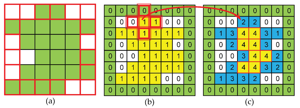
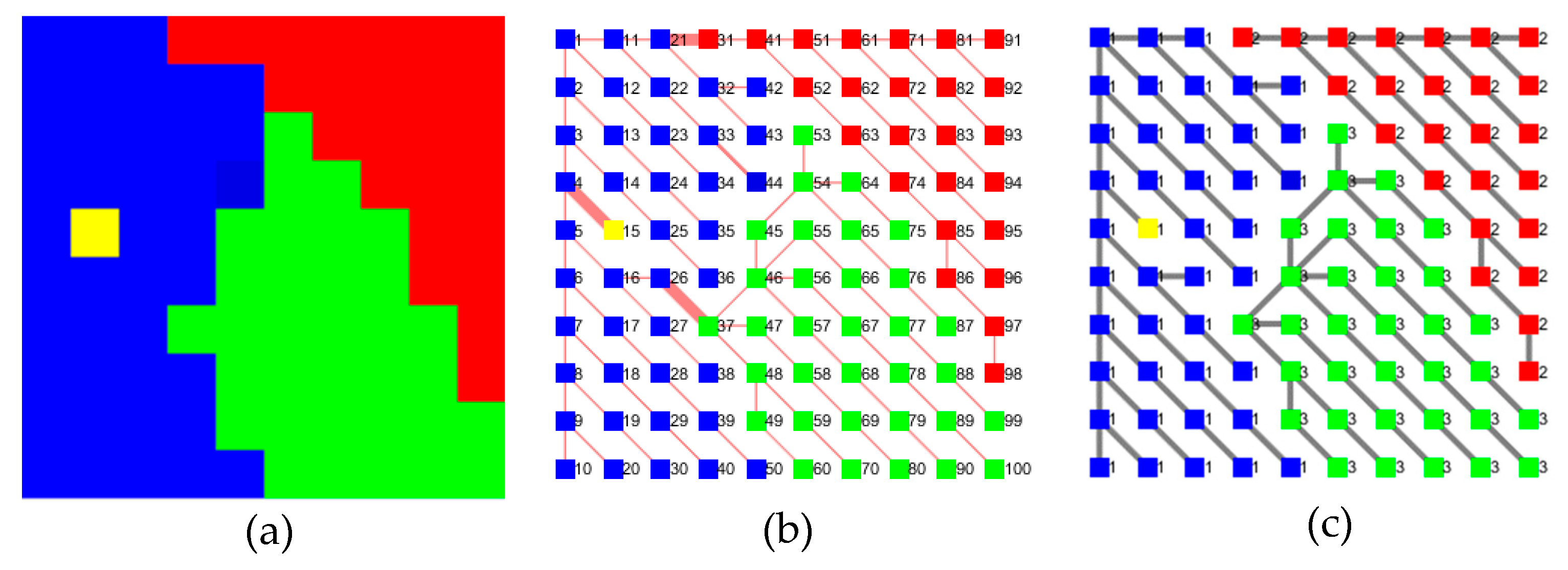
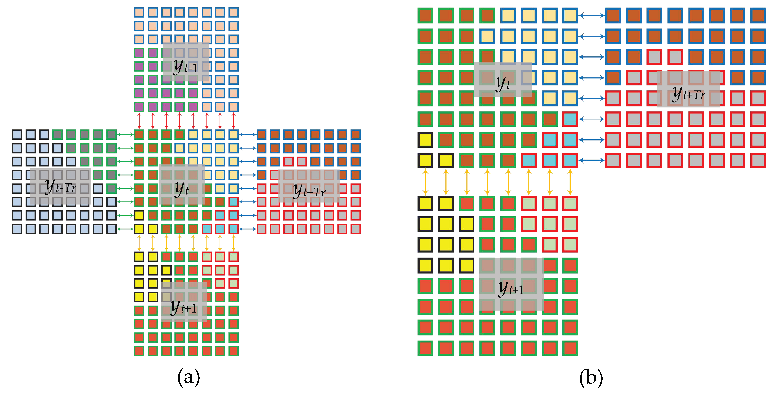
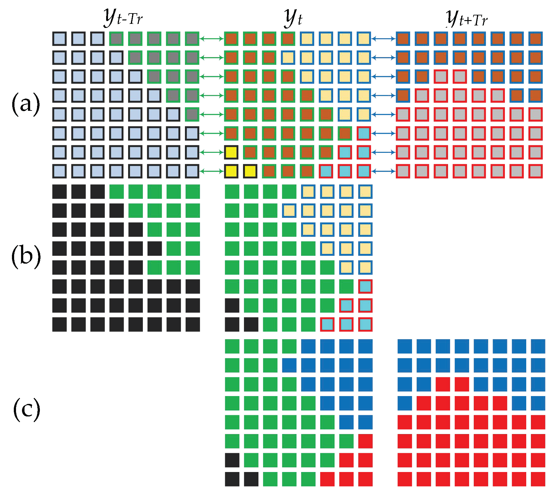
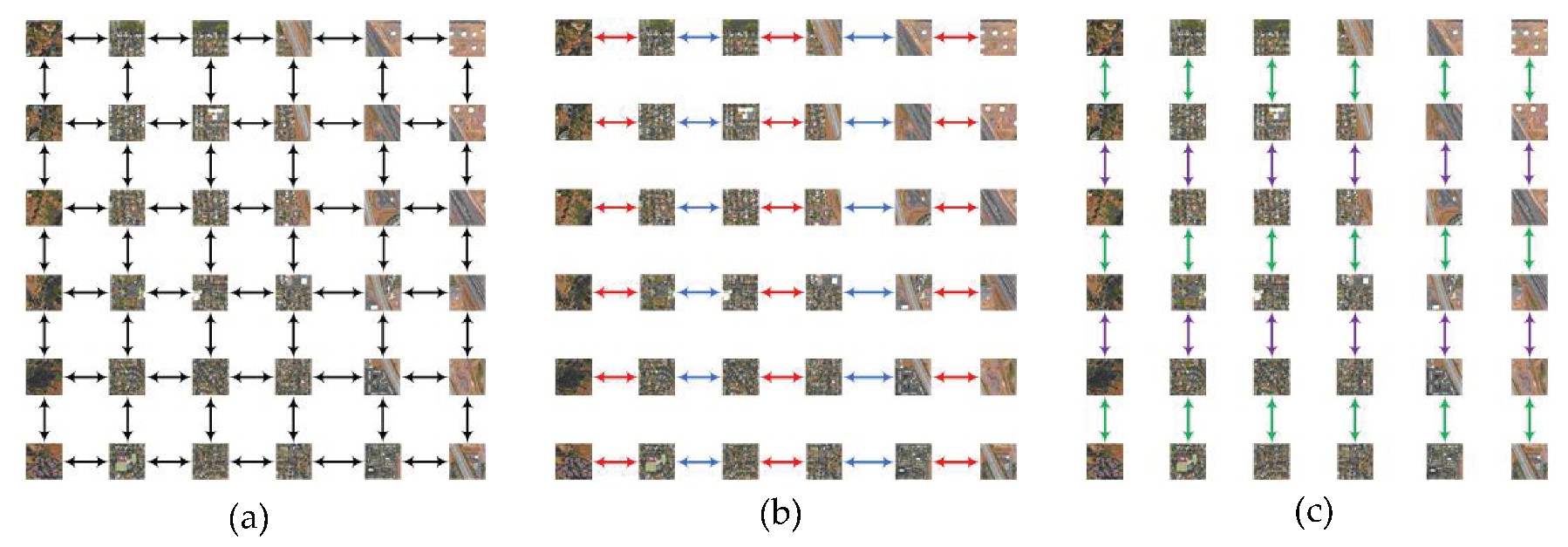
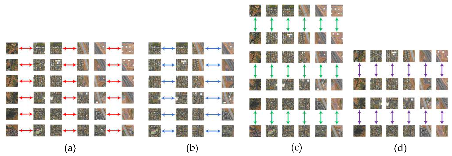
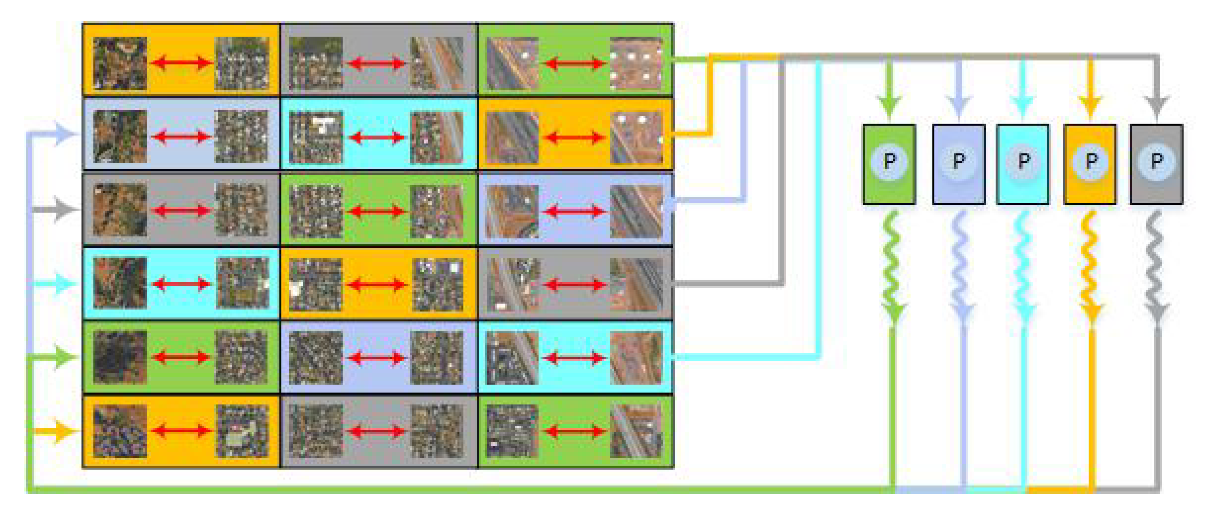
2.1.1. Block Partitioning

For subimage Z_t, its image domain F_t can be divided into I_t^S disjoint nonempty regions according to the MHR, such that, F = {F_ti; i = 1, 2, …, I_t^S}, the corresponding sub-image is Z_ti = {z_a; a = 1, 2,…, N_ti, (u_a, v_a) ∈ F_ti}, N_ti is the number of pixels in the i-th region of block t, a is the local pixel index of the i-th region of block t, S is the threshold of MHR, and each homogeneous region F_ti corresponds to a certain land use and land cover (LULC) class or part of it. In order to better express the explicit and implicit features of blocks, the MST model is used to express blocks as image minimum spanning tree field (IMSTF). Let the pixels of block be mapped to vertices, the 8-neighborhood of pixels is taken as the adjacency relationship, and the nonsimilarity measure between the spectral measure vectors between the pixels is taken as the edge weight, the block can be expressed as graph Ɠ_t = (V_t, E_t, Ψ_t), where V_t = {v_a = (u_a, v_a, z_a); a = 1, 2, …, N_t} is the vertex set, E_t = {e_c = (v_c1v_c2); c = 1, 2, …, C_t, v_c1, v_c2 ∈ V_t} is the edge set, and Ψ_t = {φ_c = φ(v_c1, v_c2); c = 1, 2, …, C_t} is the edge weights set. In order to improve the computational efficiency, each edge in E_t has to be different. Therefore, the construction method for the edge set was proposed.

As shown in Figure 1, for a vertex a ∈ ({1, 2, …, N_t − row_t}/{row_t, 2row_t, …, (col_t−1)×row_t}), which is not in the last row or column, its adjacent edge set is E_a = {(v_av_{a +1}), (v_av_{a +rowt}), (v_av_{a +rowt+1}), (v_{a +rowt}v_{a +1})}. For a vertex a ∈ {row_t, 2row_t, …, (col_t−1)×row_t} or a ∈ {(col_t−1)×row_t+1, (col_t−1)×row_t+2, …, N_t}, which is in the last row or column but not the lower right corner, its adjacent edge set is E_a = {(v_av_{a +rowt})} or E_a = {(v_av_{a +1})}, respectively. The adjacent edge set of a vertex in the lower right corner is E_a = ∅. The edge set E = {E_a; a = 1, 2, …, N_t} = {e_c = (v_c1v_c2); c = 1, 2, …, C_t, v_c1 ∈ V_t, v_c2 ∈ N_p(v_c1)}, where N_p(v_c1) is the 8-neighborhood of vertex v_c1, c is the index of edge, C_t is the number of edges, and its calculation equation as follows:

$$\begin{array}{l}{C}_t=4\left(ro{w}_t-1\right)\times \left(co{l}_t-1\right)+co{l}_t-1+ro{w}_t-1\\ \hspace{1em}=4N_t-3\left(ro{w}_t+co{l}_t\right)+2\end{array}$$

(3)

φ_c = φ(v_c1, v_c2) is defined as the nonsimilarity measure of two vertices spectral vectors connected by e_c:

$${\phi }_c=\frac{\exp \left(t_1\times d_{c1c2}\right)}{\cos \left(t_2\times {\theta }_{c1c2}\right)}$$

(4)

where d_c1c2 and θ_c1c2 are the euclidean distance and angle of the spectral vector between vertex v_c1 and v_c2, respectively. These parameters can be expressed as:

$${\theta }_{c1c2}=\arccos \left(\sqrt{\frac{{\mathit{z}}_{c1}^T{\mathit{z}}_{c2}}{\left({\mathit{z}}_{c1}^T{\mathit{z}}_{c1}\right)\times \left({\mathit{z}}_{c2}^T{\mathit{z}}_{c2}\right)}}\right)$$

(5)

$$d_{c1c2}=\sqrt{{\left({\mathit{z}}_{c1}-{\mathit{z}}_{c2}\right)}^T\left({\mathit{z}}_{c1}-{\mathit{z}}_{c2}\right)}$$

(6)

where t₁, t₂ ∈ (0,1) are the coefficients of d_c1c2 and θ_c1c2 in Equation (4), respectively. After a lot of experiments, we found that the fine results could be obtained by setting t₁ = 0.1 and t₂ = 0.8.

For the block graph Ɠ_t, the MST rule was introduced to simplify Ɠ_t, and T_t = (V_t¯, E_t¯, Ψ_t¯) was obtained. The vertex set V_t¯ = V_t, edge set E_t¯ = {e_g = (v_g1v_g2); g = 1, 2, …, N_t− 1, v_g1, v_g2 ∈ V_t¯}, and Ψ_t¯= {φ_g = φ(v_g1, v_g2); g = 1, 2, …, N_t − 1} is the set of connection weights corresponding to the connected edges. φ_g is defined by Equation (4). T_t has the following advantages:

(1).

The operation time complexity based on T_t is O(|V_t¯|), which has linear complexity.

(2).

Every edge of E_t¯ is a cut edge, such that deleting or restoring an edge will increase or decrease a region, which greatly simplifies the complexity of the partition operation, and each region corresponds to a tree.

(3).

The boundary of the target on T_t is generated along the edge, which is helpful to express the complex and irregular boundary of the target.

The classical algorithms for solving MST are the Prim [36] and Kruskal [37] algorithms, which are both based on the greedy strategy. The Prim algorithm is a vertex-driven mode with time complexity of O(|E| + |V|log|V|) based on the Fibonacci heap and is suitable for dense graphs. Kruskal algorithm is an edge-driven algorithm with time complexity of O(|E|log|E|), and is appropriate for sparse graphs. Generally speaking, the graph is called sparse graph when 0 ≤ |E| ≤ |V|log|V|. Otherwise, the graph is dense. From Equation (3), Ɠ_t is constructed by 8-neighborhood, which can be considered as a sparse graph. Thus, the solution for the block MST in this study was realized using the Kruskal algorithm.

At the start of the Kruskal algorithm, all vertices are treated as an MST. The merging tree operation by ascending order of edge weights is then defined until all MSTs are merged into one. Each merging tree operation ensures that the merged graph is a tree which does not contain any cycles. The algorithm’s greedy strategy is embodied in the order of merging, such that the edge set is rearranged in ascending order of edge weights before iteration, so the edges with small edge weights are merged early in the iteration procedure. Traditional cycle detection algorithms used by the Kruskal are inefficient because of their search strategy, e.g., disjoint set algorithm and rank-and-path compression algorithm take time complexity O(log|V|) [38,39]. For improving the performance, a new cycle detection method based on tree marker vectors was proposed, and its pseudo-code o is presented in Algorithm 1.

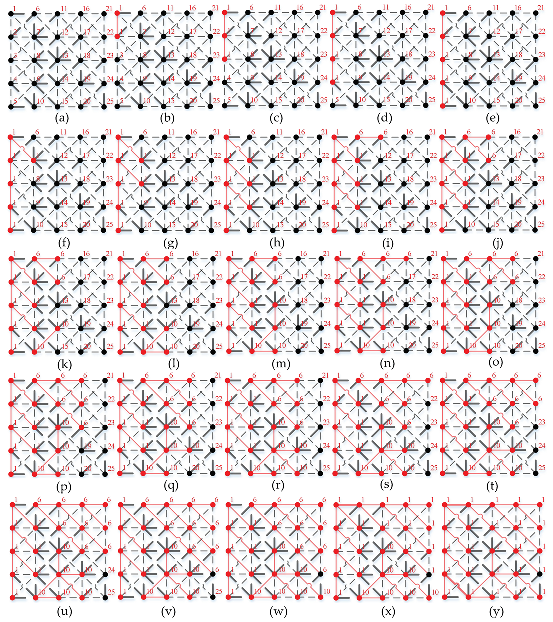
Algorithm 1. Proposed image MST generation method based on Kruskal algorithm

Input: graph Ɠt = (Vt, Et, Ψt)

Output: MST Tt = (Vt¯, Et¯, Ψt¯)

Initialization: Vt¯ = ∅, Et¯ = ∅, Ψt¯= ∅, t = {1, 2, …, |Vt¯|}

1. do Et = sortrows(Et, Ψt, “ascending”)

2. for each ec = (vc1, vc2) ∈ Et

3.  do if t(vc1) ≠ t(vc2)

4.   do Et¯ =Et¯ ∪ {ec}, Ψt¯ = Ψt¯ ∪ {φc}, Vt¯ = Vt¯∪ {vc1, vc2}, Vt¯ = unique(Vt¯)

5.   do t(t = t(vc2)) = t(vc1)// all markers of the vertices t(vc2) are changed to t(vc1)

The edge set E was rearranged in ascending order of edge weight in step 1 of Algorithm 1. The subsequent cycle judgment process (steps 4, 5) had no order operation in the edge set. Thus, the E_t¯ of the MST was strictly in the ascending order, which is an important characteristic of the Kruskal algorithm. The function unique (V_t¯) was used for removing duplicate vertices. According step 3 in Algorithm 1, the cycle detection is very simple and takes constant time complexity, which shows the efficiency of proposed method.

The iteration procedure of the proposed image MST generation method based on the Kruskal algorithm is shown in Figure 2. The red and the black points represent the vertices inside and outside of the V_t¯, respectively. The red solid lines and the black dotted lines represent the edges inside and outside of the E_t¯, respectively. The red numbers were used to show the dynamic change procedure of the tree marker vector. The tree marker vector t was used to mark which tree each vertex belongs to. In the initial stage, each vertex was considered as a tree, as shown in Figure 2a. During the iteration procedure, the merging process for trees was accomplished by changing the tree marker of the vertices. As shown in Figure 2b, both vertices 1 and 2 belong to the tree marked 1 after changing the vertex marker from 2 to 1. The judgment of cycle becomes very simple after the introduction of the tree marker vector t, which only requires the determination of whether the tree markers of the two vertices in the merging edge are the same at each iteration. If they are the same, a cycle will be introduced after the merging operation, and the operation is refused. Oherwise, the operation is accepted.

IMSTF reflects the spectral similarity and spatial clustering among pixels and expresses the explicit and implicit features of images. Essentially, it is an extension of the raster structure of image domain and explicitly depicts the connective relationship between vertices, especially its spatial clustering attribute, which has a positive effect on subsequent image processing. On this basis, in order to solve the problems of geometric noise and heterogeneity increase among homogeneous regions in high-resolution images, the similarity of spectral measures and the shape proportionality between regions were taken as the criterion for merging regions based on MHR.

Each vertex was assumed as a homogeneous region. Each edge e_g∈E_t¯ was a cut edge and was therefore regarded as the merging edge of its two connected regions. The criterion for merging regions was defined, which used the expression h(F_ti, F_ti′) ≤ S to determine whether the regions merged or not. In the expression, F_ti and F_ti′ are two regions in the block t connected by e_g. Finally, each cut edge was traversed, which was then followed by the merging procedure. The dividing scale S was used to describe the regional heterogeneity.

The merging criterion h(F_i, F_i′) is a linear combination of spectral similarity and shape proportionality between regions, and is defined as,

$$h\left({\mathit{F}}_{ti},{\mathit{F}}_{t{i}^{\prime }}\right)=\alpha h_{\mathrm{color}}+(1-\alpha )h_{\mathrm{shape}}$$

(7)

where:

$$h_{\mathrm{color}}={\displaystyle \sum _b\frac{1}{{\sigma }_b^2}\left[N_{\mathrm{merge}}{\sigma }_{b,\mathrm{merge}}-\left(N_{ti}{\sigma }_{b,ti}+N_{t{i}^{\prime }}{\sigma }_{b,t{i}^{\prime }}\right)\right]}$$

(8)

$$h_{\mathrm{shape}}=\gamma h_{\mathrm{compt}}+\left(1-\gamma \right)h_{\mathrm{smooth}}$$

(9)

$$h_{\mathrm{compt}}=l_{\mathrm{merge}}\sqrt{N_{\mathrm{merge}}}-\left(l_{ti}\sqrt{N_{ti}}+l_{t{i}^{\prime }}\sqrt{N_{t{i}^{\prime }}}\right)$$

(10)

$$h_{\mathrm{smooth}}=N_{\mathrm{merge}}\frac{l_{\mathrm{merge}}}{b_{\mathrm{merge}}}-\left(N_{ti}\frac{l_{ti}}{b_{ti}}+N_{t{i}^{\prime }}\frac{l_{t{i}^{\prime }}}{b_{t{i}^{\prime }}}\right)$$

(11)

where α ∈ [0, 1] is the coefficient of spectral similarity, and h_color is the spectral similarity. σ_b,merge, σ_b,ti, and σ_b,ti′ are the standard deviations of the spectral measure of the merged region (F_ti∪F_ti′), region ti, and ti′, respectively. N_merge, N_ti, and N_ti′ are the pixels numbers of the merged region (F_ti∪F_ti′), the region ti, and ti′, respectively. 1/σ_b² is the weight of band b and σ_b² is the variance of band b. The shape proportionality h_shape is a linear combination of the regional shape compactness h_compt and the smoothness h_smooth, and γ ∈ [0, 1] is the weight of the regional shape compactness. l_merge, l_ti, and l_ti′ are the outline lengths of the merged region (F_ti∪F_ti′), region ti, and ti′, respectively. b_merge, b_ti, and b_ti′ are the regional outer rectangular perimeters of the merged region (F_ti∪F_ti′), region ti, and ti′, respectively.

The solving procedure for the regional outer rectangular perimeter is shown in Figure 3a, where a green square represents a pixel in the region, and the regional outer rectangular perimeter is the number of red border squares. Figure 3b,c show the solving procedure of the regional outline. First, an augmented matrix was generated according to the coordinate range of the pixels of the region. As shown in Figure 3b, a green square represents an augmented pixel, and the pixel in the region is marked as 1 (see yellow squares). The element values of the four adjacent pixels were then summed up for each yellow square and used as replacement values. In Figure 3c, the yellow squares, with a value of 4, represent the interior pixels of the region, while the blue squares, with a value less than 4, represent the pixels on the regional outline. The length of the regional outline was determined by the number of blue squares.

The merging procedure is presented in Figure 4. Figure 4a,b illustrate the regional outer rectangular perimeter of two regions (b_ti and b_ti′) and the regional outline (l_ti andl_ti′) of region F_ti and F_ti′, respectively. Figure 4c shows the regional outer rectangular perimeter b_merge and regional outline l_merge of the merged region (F_ti∪F_ti′). The shape complementarity between regions F_ti and F_ti′ was good, so the shape proportionality h_shape of merged region (F_ti∪F_ti′) was low, which motivates the merging procedure of two regions (F_ti and F_ti′).

The procedure for the MHR partitioning procedure based on IMSTF is shown in Figure 5. Figure 5a is a simulated-color image, which consists of three homogeneous regions and is marked by three colors: Red, green, and blue. The blue region contains a yellow pixel, which was used to simulate geometric noise. Figure 5b is the MST of the simulated image, which was able to distinctly delineate boundaries. Figure 5c represents the forest obtained by the MHR criterion, with each tree corresponding to a homogeneous region. The MHR describes the regional structure of the image. Based on the simulation results, the MHR based on IMSTF is able to identify the irregular boundaries of the target and deal with the geometric noise effectively.

In addition, because E_t¯ is arranged in ascending order of edge weights and appears as a disordered hash in space, the smaller edge weight means two regions connected by the edge are more similar in spectral, and the more preferred these two regions will be merged. The procedure of the MHR partitioning method based on the IMSTF can be considered as a procedure for global and progressive region growth. Thus, the problem of the number and spatial distribution of initial growing seed points can be avoided, which is difficult to evade in traditional region growth algorithms. The procedure for the global progressive region growth is similar to the process of simulated annealing. In the initial stage, the regions with the most similar spectral characteristics are preferentially merged to form several pure region growth cores. After more iterations, the complex merging situation (with larger boundary weights) can be judged gradually, and the shape constraint plays a crucial role in making the region grow more compactly.

In terms of block tessellation, assuming each block is independent, each block can be processed in parallel. The parallel task pool Y = {y_t = y(Z_t, F_t); t = 1, 2, …, T} is formed by T blocks, where y(Z_t, F_t) is the task of the MHR partitioning method which includes block graph representation, block MST solution, and MHR partitioning, y_t is the result of block partitioning, and t is the task index.

The parallel computing system was made up of P parallel computing units and used to process Y parallel. Since the amount of data in each block was approximately the same, the runtime for each task can also be considered as roughly similar. Therefore, T tasks can be aggregated into P task groups in a balanced task distribution manner. Each parallel computing unit executes its allocated tasks in sequence. Assume that an image is tessellated into 256 blocks with five parallel execution units, which are represented by five color blocks, as shown in Figure 6. The tasks distributed by each parallel computing unit are shown in the grid of color blocks at the left side of Figure 6. Each color block corresponds to a thread in the execution procedure. Threads with the same color formed thread blocks, which were executed in sequence by the corresponding color computing units. After all the blocks were divided into regions, the global result was reduced according to the block index.

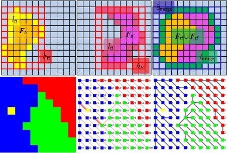
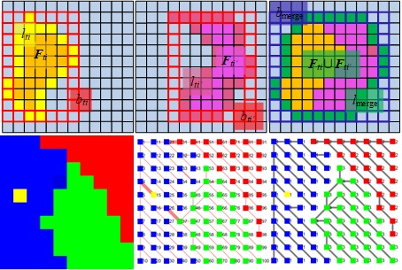
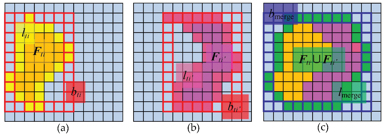
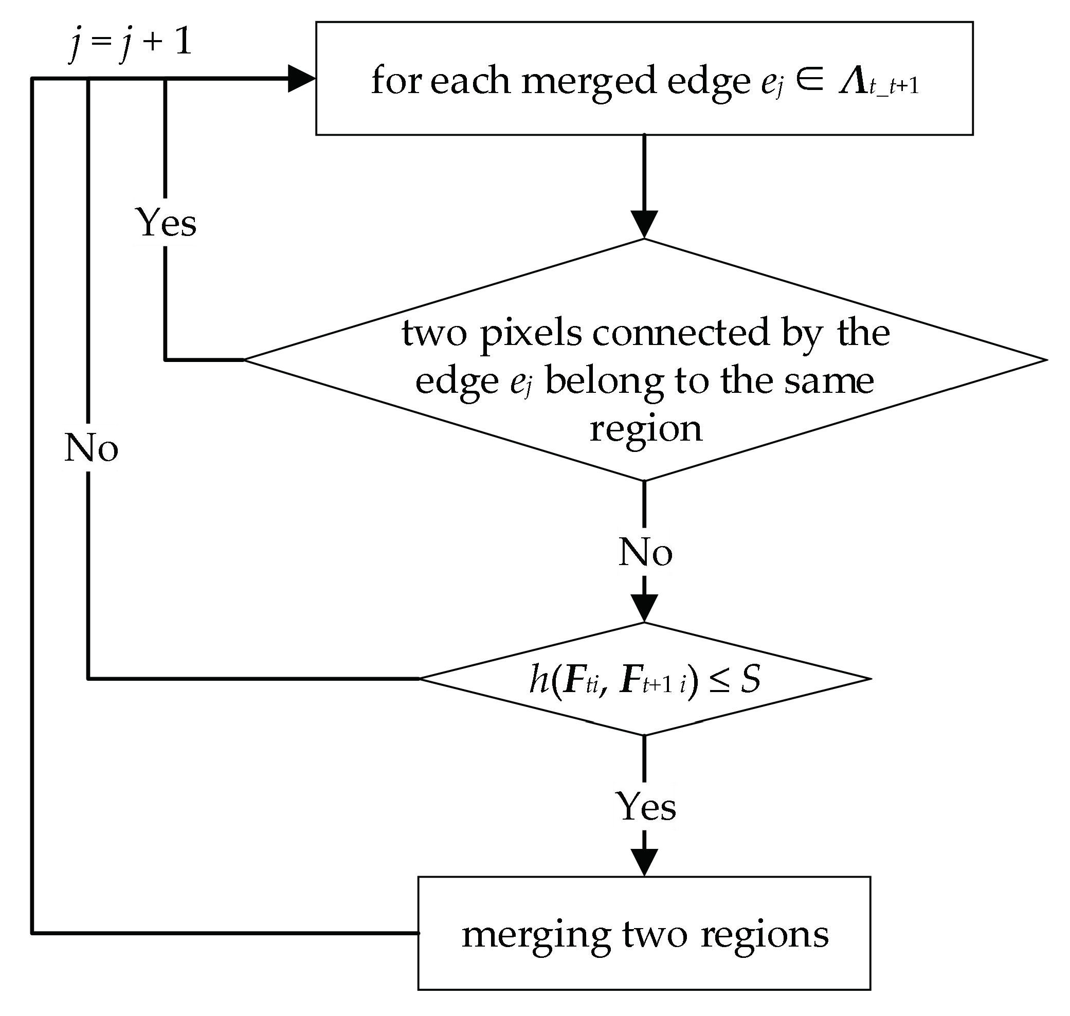
2.1.2. Block Merging

In order to decrease the damage in landscape caused by regular tessellation, the results from block paritioning had to be merged. For the resulting partition y_t of block t, its four neighborhood blocks were y_t−1, y_t+1, y_t+Tr, and y_t−Tr (see Figure 7a), where t = 1, 2, …, T, and T_r was the row number of the block. The purpose of block merging is to stitch the bordered regions by reconstructing the correlation between adjacent blocks. In merging the block y_t, the neighborhood blocks y_t−1, y_t+1, y_t+Tr, and y_t−Tr, were merged pair-wisely to avoid read-write conflicts, resulting in pairs (y_t, y_t−1), (y_t, y_t+Tr), (y_t, y_t+1), and (y_t, y_t−Tr).

Figure 7a shows the association between blocks, where the red, blue, yellow, and green bidirectional arrows indicate the associations between y_t and y_t−1, y_t+Tr, y_t+1,y_t−Tr, respectively. All bidirectional arrows identified by each color form the interblock merge set, which are represented by Λ_{t_t−1}, Λ_{t_t+Tr}, Λ_{t_t+1} and Λ_{t_t−Tr}, respectively. Each bidirectional arrow became the merge edge between two adjacent blocks, such that the red and yellow arrows were vertically correlated, while the blue and green arrows were horizontally correlated. In addition, the squares with different color bordered in Figure 7a represent different homogeneous regions, and the squares with different color fillings represent the divided regions of each block. These homogeneous regions were distributed in different blocks due to the influence of image tessellation. In effect, there was a redundancy problem in the merging procedure. For example, for the block y_t, its left block y_t−Tr and upper block y_t−1 were merged, with the center on block y_t−Tr-1. To avoid this, the actual merging procedure only needed to consider the merging of the central block with its right and lower blocks, as shown in Figure 7b. For the last row or the last column of blocks, only the right and lower blocks had to be merged with the central block (i.e., the lower right block did not need to be merged).

Figure 8 shows the dependence relationship of horizontal interblock merging. For the three blocks y_t−Tr, y_t and y_t+Tr, as shown in Figure 8a, the merged result of (y_t−Tr, y_t) was considered as input for the merging procedure of (y_t, y_t+Tr), which means that the merging result of (y_t, y_t+Tr) shown in Figure 8c depends on the merged result of (y_t−Tr, y_t) shown in Figure 8b. This dependence relationship created difficulties for the parallel merging procedure, which made it necessary to design a better parallel scheduling scheme to decouple the dependence relationship. The dependence relationship of the vertical merging process was similar to the horizontal procedure and is not discussed here.

The merging procedure of blocks can be summarized as follows: For each merged edge in Λ_{t_t+1}, if two pixels connected by the edge belong to the same region, continue on with the next merged edge. Otherwise, determine whether or not to merge these two regions based on the equation h(F_ti, F_{t+1 i}) ≤ S. If the criterion is satisfied, the two regions are merged. Otherwise, move on to the next merging edge. The flowchart of the algorithm is shown in Figure 9. Using the same principle, the merging set Λ_{t_t+Tr} was assessed, then the process was continued until all blocks were merged.

Since the merging procedure was carried out serially, when the number of blocks is large, the required processing time will be enormous. To further improve the speed of merging, a hierarchical parallel scheduling method was proposed. The computational dependency diagram for merging blocks is shown in Figure 10a. The computational dependency diagram can be divided into two parts according to the horizontal and vertical merging modes, as shown in Figure 10b,c, respectively. The red bidirectional arrow in Figure 10b indicates a horizontal first layer merging procedure, and the blue bidirectional arrow denotes a horizontal second layer merging procedure. Similarly, the green bidirectional arrow indicates a vertical first layer merging procedure, and the purple bidirectional arrow denotes a vertical second layer merging procedure.

The horizontal and vertical merging tasks of Figure 10b,c can be aggregated into the form presented in Figure 11, where Figure 11a,b are the first and second horizontal merging task sets and Figure 11c,d are the first and second vertically merging task sets, respectively. The index sets MI₁, MI₂, MI₃, and MI₄ are the block pairs of the first horizontal layer, second horizontal layer, first vertical layer, and second vertical layer, respectively. These index sets can be obtained by the following equations:

$$\mathit{M}{\mathit{I}}_1=\{\begin{array}{l}{\displaystyle \underset{r=1}{\overset{T_r}{\cup }}{\displaystyle \underset{c=1}{\overset{\frac{T_c}{2}}{\cup }}\left\{\left(2\left(c-1\right)T_r+r,\left(2c-1\right)T_r+r\right)\right\}}}, \mathrm{if} \mathrm{mod}(T_c,2)=0\\ {\displaystyle \underset{r=1}{\overset{T_r}{\cup }}{\displaystyle \underset{c=1}{\overset{\frac{T_c-1}{2}}{\cup }}\left\{\left(2\left(c-1\right)T_r+r,\left(2c-1\right)T_r+r\right)\right\}}}, \mathrm{else}\end{array}$$

(12)

$$\mathit{M}{\mathit{I}}_2=\{\begin{array}{l}{\displaystyle \underset{r=1}{\overset{T_r}{\cup }}{\displaystyle \underset{c=1}{\overset{\frac{T_c}{2}-1}{\cup }}\left\{\left(\left(2c-1\right)T_r+r,2c{T}_r+r\right)\right\}}}, \mathrm{if} \mathrm{mod}(T_c,2)=0\\ {\displaystyle \underset{r=1}{\overset{T_r}{\cup }}{\displaystyle \underset{c=1}{\overset{\frac{T_c-1}{2}}{\cup }}\left\{\left(\left(2c-1\right)T_r+r,2c{T}_r+r\right)\right\}}}, \mathrm{else}\end{array}$$

(13)

$$\mathit{M}{\mathit{I}}_3=\{\begin{array}{l}{\displaystyle \underset{c=1}{\overset{T_c}{\cup }}{\displaystyle \underset{r=1}{\overset{\frac{T_r}{2}}{\cup }}\left\{\left(\left(c-1\right)T_r+2r-1,\left(c-1\right)T_r+2r\right)\right\}}}, \mathrm{if} \mathrm{mod}(T_r,2)=0\\ {\displaystyle \underset{c=1}{\overset{T_c}{\cup }}{\displaystyle \underset{r=1}{\overset{\frac{T_r-1}{2}}{\cup }}\left\{\left(\left(c-1\right)T_r+2r-1,\left(c-1\right)T_r+2r\right)\right\}}}, \mathrm{else}\end{array}$$

(14)

$$\mathit{M}{\mathit{I}}_4=\{\begin{array}{l}{\displaystyle \underset{c=1}{\overset{T_c}{\cup }}{\displaystyle \underset{r=1}{\overset{\frac{T_r}{2}-1}{\cup }}\left\{\left(\left(c-1\right)T_r+2r,\left(c-1\right)T_r+2r+1\right)\right\}}}, \mathrm{if} \mathrm{mod}(T_r,2)=0\\ {\displaystyle \underset{c=1}{\overset{T_c}{\cup }}{\displaystyle \underset{r=1}{\overset{\frac{T_r-1}{2}}{\cup }}\left\{\left(\left(c-1\right)T_r+2r,\left(c-1\right)T_r+2r+1\right)\right\}}}, \mathrm{else}\end{array}$$

(15)

where T_r and T_c are the row and column numbers of the block, respectively, u = mod(a, b) is the remainder function, a is the dividend, b is the divisor, and u is the remainder. a, b, and u are all integers.

In terms of the aggregated result of the horizontal and vertical merging tasks, the optimized procedure can be realized using a multithread parallel execution mode. Figure 12 presents a horizontal first-level merging parallel scheduling schematic diagram. Five colors represent the five parallel execution units, each of which corresponds to a thread in the execution procedure. Thread blocks with the same color were executed serially by the corresponding color computing units. Horizontal second layer merging, vertical first layer merging, and longitudinal second layer merging were carried out in similar fashion. After all the block merging tasks were completed, the final global results were obtained by reducing according to the corresponding block index.

2.2. Regional Hidden Markov Random Field–Fuzzy C-Means (RHMRF-FCM) Segmentation

The parallel MHR partitioning procedure divides the image domain into regions. However, these regions are optimal locally and not necessarily optimal globally. Thus, the general segmentation algorithms need to adopt an additional clustering process to obtain global optimal segmentation results. In this section, the RHMRF model was developed based on the idea of pixel HMRF-FCM image segmentation and using the region as the basic decisionmaking unit.

2.2.1. RHMRF-FCM Segmentation

The image domain F was divided into I^S homogeneous regions using a parallel MHR partitioning method, such that F = {F_i; i = 1, 2, …, I^S} is the set of pixels corresponding to each region Z_i = {z_a; a = 1, 2,…, N_i}, and its label set is L = {L_i; i = 1, 2, …, I^S}. Then, the objective function of regionalized HMRF-FCM [40] can be written as:

$$F_{\lambda }\left(\mathit{R},\mathbf{\theta },\mathbf{\eta }|I^S,K\right)={\displaystyle \sum _{i=1}^{I^S}{\displaystyle \sum _{k=1}^K{r}_{ik}{D}_{ik}}}+\lambda {\displaystyle \sum _{i=1}^{I^S}{\displaystyle \sum _{k=1}^K{N}_i}}{r}_{ik}\log \left(\frac{r_{ik}}{{\eta }_{ik}}\right)$$

(16)

where the first term on the right side (Equation (16)) is the linear weighted sum of information and its fuzzy relations with all the regions, which indicates the cost of label configuration and is the main factor for clustering decisionmaking. The second term refers to the regularization of KL divergence information. It introduces the relationship between the fuzzy relation and the local label of the region, which is the expression of the region’s local constraints and can restrain the over-segmentation. λ ∈ [0,1] is the fuzzy degree, which is used to coordinate the relationship between two decision items. R = {r_ik; i = 1, 2, …, I^S, k = 1,2, …, K} is a fuzzy membership set, where r_ik describes the degree which region i belongs to the j-th cluster, and η = {η_ik; i = 1, 2, …, I^S, k = 1,2, …, K} is a prior distribution of HMRF model. η_ik is the pointwise prior probability of the RHMRF model states [41], which can be expressed as:

$${\eta }_{ik}=p\left(L_i=k|L_{i^{\prime }},{\mathit{F}}_{i^{\prime }}\in N{F}_i,\beta \right)=\frac{\exp \left(-\beta {\displaystyle \sum _{{\mathit{F}}_{i^{\prime }}\in N{F}_i}t(L_i,L_{i^{\prime }})}\right)}{{\displaystyle \sum _{k^{\prime }=1}^K\exp \left(-\beta {\displaystyle \sum _{{\mathit{F}}_{i^{\prime }}\in N{F}_i}t(L_i=k^{\prime },L_{i^{\prime }})}\right)}}$$

(17)

where NF_i is the neighborhood relationship of the region F_i, i′ is the neighborhood region index of F_i, k is the labeled index, and β ∈ [0, 1] is a parameter of the clique potentials known as the inverse supercritical temperature. t(L_i, L_i′) is the indicator function, where t(L_i, L_i′) = 1 if and only if L_i = L_i′; otherwise, t(L_i, L_i′) = 0. D_ik is the information about the class k in the data of region i and can be defined as:

$$\begin{array}{l}{D}_{ik}=-\log N\left({\mathit{Z}}_i;{\mathit{\mu }}_k,{\mathit{\Sigma }}_k\right)=-{\displaystyle \sum _{a=1}^{N_i}\log N\left({\mathit{z}}_a;{\mathit{\mu }}_k,{\mathit{\Sigma }}_k\right)}\\ =-{\displaystyle \sum _{a=1}^{N_i}\log \left\{{\left(2\pi \right)}^{-\frac{B}{2}}{\left|{\mathit{\Sigma }}_k\right|}^{\frac{1}{2}}\exp \left[-\frac{{\left({\mathit{z}}_a-{\mathit{\mu }}_k\right)}^T{\mathit{\Sigma }}_k^{-1}\left({\mathit{z}}_a-{\mathit{\mu }}_k\right)}{2}\right]\right\}}\\ \Rightarrow D_{ik}=-\frac{N_i}{2}\left[B\log 2\pi +\log \left|{\mathit{\Sigma }}_k\right|\right]-\frac{1}{2}{\displaystyle \sum _{a=1}^{N_i}{\left({\mathit{z}}_a-{\mathit{\mu }}_k\right)}^T{\mathit{\Sigma }}_k^{-1}\left({\mathit{z}}_a-{\mathit{\mu }}_k\right)}\end{array}$$

(18)

where θ = {θ_k = {μ_k, ∑_k}; k = 1, 2, …, K} is the set of model parameters, μ_k is the mean vector with B dimension, and ∑_k is the covariance matrix with B×B dimension. The global optimal segmentation result based on region partitioning is the minimum solution of the objective function (Equation (16)). The explicit class attributes of each region can be obtained by de-fuzzifying the fuzzy relation matrix R. At present, defuzzification is usually solved by maximizing the fuzzy relation, such that:

$$L_i=\underset{k}{\arg \max }\left\{r_{ik};k=1,2,\dots ,K\right\}$$

(19)

By substituting Equations (17) and (18) into Equation (16), the final form of the objective function was obtained:

$$\begin{array}{l}{F}_{\lambda }\left(\mathit{R},\mathbf{\theta },\mathbf{\eta }|I^S,K\right)\\ =-{\displaystyle \sum _{i=1}^{I^S}{\displaystyle \sum _{k=1}^K{r}_{ik}\left\{\frac{N_i}{2}\left[B\log 2\pi +\log \left|{\mathit{\Sigma }}_k\right|\right]+\frac{1}{2}{\displaystyle \sum _{a=1}^{N_i}{\left({\mathit{z}}_a-{\mathit{\mu }}_k\right)}^T{\mathit{\Sigma }}_k^{-1}\left({\mathit{z}}_a-{\mathit{\mu }}_k\right)}\right\}}}+\lambda {\displaystyle \sum _{i=1}^{I^S}{\displaystyle \sum _{k=1}^K{N}_i}}{r}_{ik}\log \left(\frac{r_{ik}}{{\eta }_{ik}}\right)\end{array}$$

(20)

where μ_k, ∑_k, and r_ik are unknown parameters. μ_k and ∑_k are explicit parameters, such that the partial derivatives of the objective function for these two parameters can be solved by the following equations:

$$\frac{\partial F_{\lambda }}{\partial {\mathit{\mu }}_k}=0\Rightarrow {\mathit{\mu }}_k=\frac{{\displaystyle \sum _{i=1}^{I^S}{r}_{ik}{\displaystyle \sum _{a=1}^{N_i}{\mathit{z}}_a}}}{{\displaystyle \sum _{i=1}^{I^S}{N}_i{r}_{ik}}}$$

(21)

$$\begin{array}{l}\frac{\partial F_{\lambda }}{\partial {\mathit{\Sigma }}_k}=0\Rightarrow {\displaystyle \sum _{i=1}^{I^S}{r}_{ik}\frac{N_i}{2}\left(-{\mathit{\Sigma }}_k^{-1}\right)}+{\displaystyle \sum _{i=1}^{I^S}{r}_{ik}{\displaystyle \sum _{a=1}^{N_i}\frac{1}{2}{\mathit{\Sigma }}_k^{-1}{\left({\mathit{z}}_a-{\mathit{\mu }}_k\right)}^T\left({\mathit{z}}_a-{\mathit{\mu }}_k\right){\mathit{\Sigma }}_k^{-1}}}=0\\ \Rightarrow {\mathit{\Sigma }}_k=\frac{{\displaystyle \sum _{i=1}^{I^S}{r}_{ik}{\displaystyle \sum _{a=1}^{N_i}{\left({\mathit{z}}_a-{\mathit{\mu }}_k\right)}^T\left({\mathit{z}}_a-{\mathit{\mu }}_k\right)}}}{{\displaystyle \sum _{i=1}^{I^S}{N}_i{r}_{ik}}}\end{array}$$

(22)

where ∂log|Σ_k|/∂ Σ_k = $-{\mathit{\Sigma }}_k^{-1}, \partial {\left({\mathit{z}}_a-{\mathit{\mu }}_k\right)}^T{\mathit{\Sigma }}_k^{-1}\left({\mathit{z}}_a-{\mathit{\mu }}_k\right)$/∂ Σ_k =${\mathit{\Sigma }}_k^{-1}{\left({\mathit{z}}_a-{\mathit{\mu }}_k\right)}^T\left({\mathit{z}}_a-{\mathit{\mu }}_k\right){\mathit{\Sigma }}_k^{-1}$.

The fuzzy membership r_ik satisfies the constraint condition ∑_kr_ik = 1, such that the sum of the fuzzy relations of a region belonging to all classes is equal to 1. Therefore, a Lagrange function was constructed to solve the problem based on the constraints,

$$f\left(r_{i1},r_{i2},\dots ,r_{iK}\right)={\displaystyle \sum _{k=1}^K{r}_{ik}{D}_{ik}}+\lambda {\displaystyle \sum _{k=1}^K{N}_i{r}_{ik}\log \left(\frac{r_{ik}}{{\eta }_{ik}}\right)}+{\xi }_i\left({\displaystyle \sum _{k=1}^K{r}_{ik}}-1\right)$$

(23)

Let the partial derivative of f(r_i1, r_i2, …, r_iK) to r_ik be 0,

$$\begin{array}{l}\frac{\partial f\left(r_{i1},r_{i2},\dots ,r_{iK}\right)}{\partial r_{ik}}=0\\ \Rightarrow D_{ik}+\lambda N_i\left[\log \left(\frac{r_{ik}}{{\eta }_{ik}}\right)+r_{ik}\frac{{\eta }_{ik}}{r_{ik}}\frac{1}{{\eta }_{ik}}\right]+{\xi }_i=0\end{array}$$

(24)

$$\Rightarrow r_{ik}=\exp \left(-\frac{{\xi }_i}{\lambda N_i}+1\right){\eta }_{ik}\exp \left[-\frac{D_{ik}}{\lambda N_i}\right]$$

(25)

As

$${\displaystyle \sum _{k^{\prime }=1}^K{r}_{i{k}^{\prime }}}=1\Rightarrow {\displaystyle \sum _{k^{\prime }=1}^K{\eta }_{i{k}^{\prime }}\exp \left[-\frac{D_{i{k}^{\prime }}}{\lambda N_i}\right]\exp \left(-\frac{{\xi }_i}{\lambda N_i}+1\right)}=1$$

(26)

$$\Rightarrow 1=\exp \left(-\frac{{\xi }_i}{\lambda N_i}+1\right){\displaystyle \sum _{k^{\prime }=1}^K{\eta }_{i{k}^{\prime }}\exp \left[-\frac{D_{i{k}^{\prime }}}{\lambda N_i}\right]}$$

(27)

Equation (28) was obtained by taking Equation (25) divided by Equation (27),

$$r_{ik}=\frac{{\eta }_{ik}\exp \left(-\frac{1}{\lambda N_i}{D}_{ik}\right)}{{\displaystyle \sum _{k^{\prime }=1}^K{\eta }_{i{k}^{\prime }}\exp \left(-\frac{1}{\lambda N_i}{D}_{i{k}^{\prime }}\right)}}$$

(28)

Equation (29) was obtained by substituting Equation (18) into Equation (28),

$$r_{ik}=\frac{{\eta }_{ik}\exp \left(\frac{1}{2\lambda }\log \left|{\mathit{\Sigma }}_k\right|+\frac{1}{2\lambda N_i}{\displaystyle \sum _{a=1}^{N_i}{\left({\mathit{z}}_a-{\mathit{\mu }}_k\right)}^T{\mathit{\Sigma }}_k^{-1}\left({\mathit{z}}_a-{\mathit{\mu }}_k\right)}\right)}{{\displaystyle \sum _{k^{\prime }=1}^K{\eta }_{i{k}^{\prime }}\exp \left(\frac{1}{2\lambda }\log \left|{\mathit{\Sigma }}_{k^{\prime }}\right|+\frac{1}{2\lambda N_i}{\displaystyle \sum _{a=1}^{N_i}{\left({\mathit{z}}_a-{\mathit{\mu }}_{k^{\prime }}\right)}^T{\mathit{\Sigma }}_{k^{\prime }}^{-1}\left({\mathit{z}}_a-{\mathit{\mu }}_{k^{\prime }}\right)}\right)}}$$

(29)

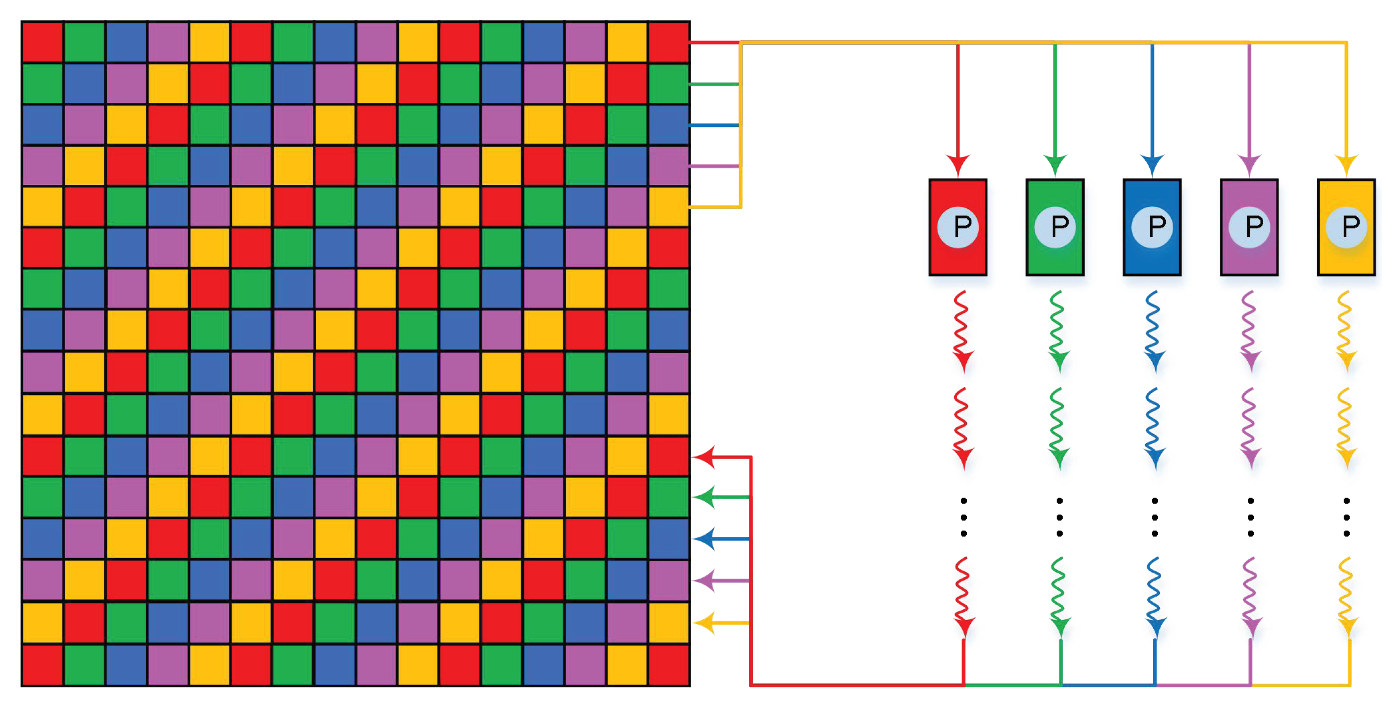
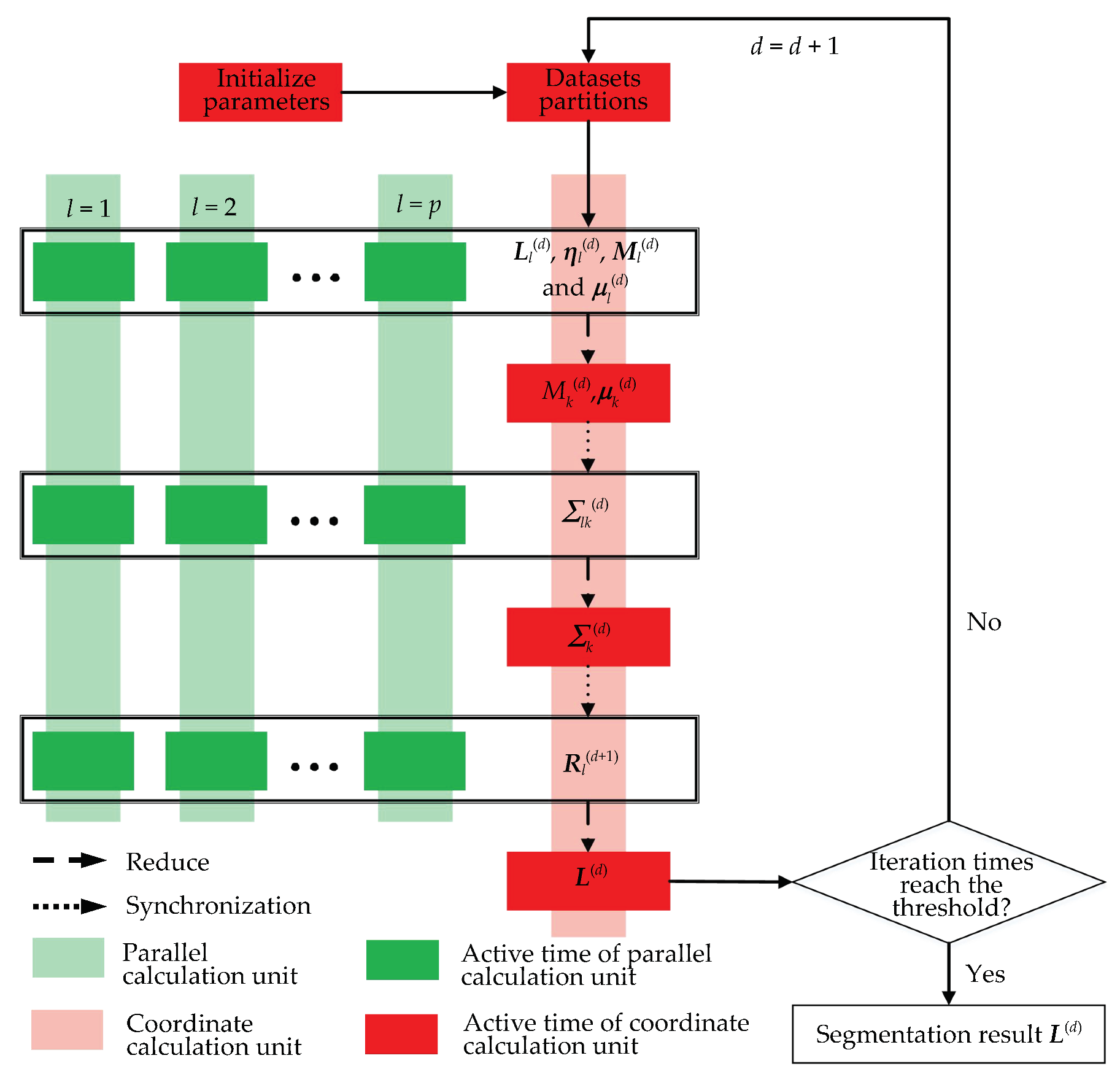
2.2.2. Parallel RHMRF-FCM Segmentation

When the number of pixels is huge, or the image information is complex, the number of regions generated will also be very large, which leads to protracted runtime of the serial RHMRF-FCM algorithm. In addition, for multicore parallel computing systems, the communication time between cores is extremely expensive. Effectively reducing the amount of data synchronization can significantly improve the performance of parallel algorithms [42]. Therefore, a parallel RHMRF-FCM algorithm was proposed based on a master-slave parallel mode. The algorithm is described in detail as follows.

For a parallel computing system consisting of P parallel computing units and a coordinated computing unit, in order to make full use of computing performance brought by parallel computing, the dataset Z was equally partitioned into P subsets according to the number of regions, such that Z = {Z_l; l = 1, 2, …, p}. Z_l = {Z_lq; q = 1, 2, …, N_l} is the l-th subset data, Z_lq = {z_lqa; a = 1, 2, …, N_q} is the data of region q in the subsetl, a is the pixel index of region q, and z_lqa is the spectral measure of pixel a in the region q of subsetl. N_l is the number of regions in subset l, which can be computed as:

$$N_l=\{\begin{array}{l}\lceil \frac{I}{p}\rceil ,l=1,2,\dots ,p-1\\ I-\left(p-1\right)\lceil \frac{I}{p}\rceil ,l=p\end{array}$$

(30)

Similarly, other local variables in the calculation process were defined according to the same rules. The partition of neighborhood regions index set is U = {U_l; l = 1, 2, …, p}, where U_l = {NF_lq; q = 1, 2, …, N_l} is the l-th subset of neighborhood regions index set. The partition of prior distribution region labels is η = {η_l; l = 1, 2, …, p}, where the l-th subset is η_l = {η_lq = {η_lqk; k = 1, 2, …, K; q = 1, 2, …, N_l}. The partition of region label set is L = {L_l; l = 1, 2, …, p}, where the l-th subset is L_l = {L_lq ∈ {1, 2, …, K}; q = 1, 2, …, N_l}. M = {M_l = {M_lk; k = 1, 2, …, K}; l = 1, 2, …, p} is a temporary variable introduced to facilitate parallel computing, θ = {θ_l; l = 1, 2, …, p } is a clustering parameter, the l-th subset is θ_l = {(μ_lk, ∑_lk); k = 1, 2, …, K}, and μ_lk and ∑_lk are the mean vector and covariance matrix of class k in the l-th subset, respectively. The partition of region fuzzy membership set is R = {R_l; l = 1, 2, …, p}, given the l-th subset is R_l = {R_lq = {r_lqk; k = 1, 2, …, K}; q = 1, 2, …, N_l}.

By the master-slave parallel mode, the flow of the parallel RHMRF-FCM algorithm can be summarized as follows:

(1) Initialization algorithm parameters include the iteration index d = 0, clustering number K, fuzzy degree λ, and iteration threshold T. Initiate the p parallel computing units and the coordinated computing unit. The p parallel computing units are responsible for the calculation of p subsets of corresponding data sets, while the coordination computing unit is responsible for the dataset partitioning and the allocation of the local parameters.

(2) Coordinate computing unit for data partition and data transmission include the partition data set Z_l = {Z_lq; q = 1, 2, …, N_l}. Randomly initialize and partition the region fuzzy membership set R^(d) = {R_l^(d); l = 1, 2, …, p}. Compute and divide the neighborhood region index set U = {U_l; l = 1, 2, …, p}, then transmit the partitioned data sets Z_l, R_l^(d,⁾ and U_l to the corresponding threads.

(3) Compute, in parallel, each label field subset L_l^(d) = {L_lq^(d); q = 1, 2, …, N_l}, prior distribution η_l^(d) = {η_lq^(d) = {η_lqk^(d); k = 1, 2, …, K}}, M_l^(d) = {M_lk^(d); k = 1, 2, …, K}, and μ_l^(d) = {μ_lk^(d); k = 1, 2, …, K} on p computation units. Calculate L_lq^(d), η_lqk^(d), M_lk^(d), and μ_lk^(d) in parallel threads successively by executing the following equations:

$${\mathit{L}}_{lq}^{\left(d\right)}=\underset{k}{\arg \max }\left\{r_{lqk}^{\left(d\right)};k=1,2,\dots ,K\right\}$$

(31)

$${\eta }_{lqk}^{\left(d\right)}=\frac{\exp \left(-\beta {\displaystyle \sum _{{\mathit{F}}_{q^{\prime }}\in N{F}_{lq}}t\left({\mathit{L}}_{lq}^{\left(d\right)}=k,{\mathit{L}}_{q^{\prime }}^{\left(d\right)}\right)}\right)}{{\displaystyle \sum _{k^{\prime }=1}^K\exp \left(-\beta {\displaystyle \sum _{{\mathit{F}}_{q^{\prime }}\in N{F}_{lq}}t\left({\mathit{L}}_{lq}^{\left(d\right)}=k^{\prime },{\mathit{L}}_{q^{\prime }}^{\left(d\right)}\right)}\right)}}$$

(32)

$$M_{lk}^{\left(d\right)}={\displaystyle \sum _{q=1}^{N_l}{N}_q{r}_{lqk}^{\left(d\right)}}$$

(33)

$${\mathit{\mu }}_{lk}^{\left(d\right)}={\displaystyle \sum _{q=1}^{N_l}{r}_{lqk}^{\left(d\right)}{\displaystyle \sum _{a=1}^{N_q}{\mathit{z}}_{lqa}}}$$

(34)

(4) Reduce M_l^(d) and μ_l^(d) using the coordinate computing unit from p computation units, and calculate M_k^(d) and μ_k^(d) using Equations (35) and (36). Then, synchronize the parametersM_k^(d) and μ_k^(d) to p parallel computing units.

$$M_k^{\left(d\right)}={\displaystyle \sum _{l=1}^p{M}_{lk}^{\left(d\right)}}$$

(35)

$${\mathit{\mu }}_k^{\left(d\right)}=\frac{{\displaystyle \sum _{l=1}^q{\mathit{\mu }}_{lk}^{\left(d\right)}}}{M_k^{\left(d\right)}}$$

(36)

(5) Compute ∑_l^(d) = {∑_lk^(d); k = 1, 2, …, K} using p parallel computing units by:

$${\mathit{\Sigma }}_{lk}^{\left(d\right)}=\frac{{\displaystyle \sum _{q=1}^{N_l}{r}_{lqk}^{\left(d\right)}{\displaystyle \sum _{a=1}^{N_q}{\left({\mathit{z}}_{lqa}-{\mathit{\mu }}_k^{\left(d\right)}\right)}^T\left({\mathit{z}}_{lqa}-{\mathit{\mu }}_k^{\left(d\right)}\right)}}}{M_k^{\left(d\right)}}$$

(37)

(6) Reduce ∑_l^(d) from p computation units, and calculate the ∑_k^(d) by Equation (38). Then, synchronize the ∑_k^(d) to p parallel computational units:

$${\mathit{\Sigma }}_k^{\left(d\right)}={\displaystyle \sum _{l=1}^q{\mathit{\Sigma }}_{lk}^{\left(d\right)}}$$

(38)

(7) Compute R_l^(d+1) = {R_lq^(d+1) = {r_lqk^(d+1); k = 1, 2, …, K}; q = 1, 2, …, N_l} in p parallel computing units using the equation:

$$r_{lqk}^{\left(d+1\right)}=\frac{{\eta }_{lqk}^{\left(d\right)}\exp \left(\frac{1}{2\lambda }\log \left|{\mathit{\Sigma }}_k^{\left(d\right)}\right|+\frac{1}{2\lambda N_q}{\displaystyle \sum _{a=1}^{N_q}{\left({\mathit{z}}_{lqa}-{\mathit{\mu }}_k^{\left(d\right)}\right)}^T{\left({\mathit{\Sigma }}_k^{\left(d\right)}\right)}^{-1}\left({\mathit{z}}_{lqa}-{\mathit{\mu }}_k^{\left(d\right)}\right)}\right)}{{\displaystyle \sum _{k^{\prime }=1}^K{\eta }_{lq{k}^{\prime }}^{\left(d\right)}\exp \left(\frac{1}{2\lambda }\log \left|{\mathit{\Sigma }}_{k^{\prime }}^{\left(d\right)}\right|+\frac{1}{2\lambda N_q}{\displaystyle \sum _{a=1}^{N_q}{\left({\mathit{z}}_{lqa}-{\mathit{\mu }}_{k^{\prime }}^{\left(d\right)}\right)}^T{\left({\mathit{\Sigma }}_{k^{\prime }}^{\left(d\right)}\right)}^{-1}\left({\mathit{z}}_{lqa}-{\mathit{\mu }}_{k^{\prime }}^{\left(d\right)}\right)}\right)}}$$

(39)

(8) If the iterations threshold is reached, the partition result L^(d) is reduced and the loop is withdrawn. Otherwise, d = d+1, and then return to step (3) in the iteration process.

In order to more clearly define the local parallel computation, the parallel RHMRF-FCM algorithm was reduced and synchronized. The flowchart of the algorithm is shown in Figure 13. The local variables in each parallel computing unit were Z_l, U_l, R_l, L_l, η_l, M_l, and θ_l. The variables stored in the computation procedure of the coordinated computing unit were M_k, μ_k, and ∑_k. As shown in Figure 13, the parallel computing units were responsible for the calculation of parameters related to data and the main computing carriers of the algorithm. The coordination computing unit was responsible for the generation of local parameters, the calculation of global parameters, and the synchronization of global parameters to each parallel computing unit. In addition, the parallel RHMRF-FCM algorithm only needed to specify and synchronize the global model parameters, which mainly included M_l^(d), μ_l^(d), and ∑_l^(d). The synchronization parameters mainly included M_k^(d), μ_k^(d), and ∑_k^(d). Based on the definition of the parameters, the amount of data of these parameters was only linearly related to the number of parallel computing units p, resulting in the algorithm being a parallel scheme with low data traffic.

3. Results and Discussion

Our previous works (serial method), presented in Reference [10], discussed the influence of the parameters of serial MHR partitioning method to the final segmentation result, obtained available range of parameters, and compared the multiresolution and watershed segmentation method of the eCognition software, so we will not be repeatedly discussing them. In this study, we focused on the discussion of the cost of the parallel segmentation method and parallel performance analysis. The cost analysis was mainly concerned with the impact of the proposed parallel segmentation schemes on global segmentation results under different data tessellation scales and was evaluated qualitatively and quantitatively. The parallel performance analysis involved the assessment of runtime and speedup [43] of parallel MHR partitioning, parallel regionalization segmentation, and the proposed segmentation method with different cores.

3.1. Cost Analysis

In order to qualitatively and quantitatively evaluate the influence of block tessellation on the proposed parallel segmentation method, a WorldView-3 Pan-Sharpen multi-band image with 1024 × 1024 pixels and spatial resolution of 0.5 m was used as the experimental image (see Figure 14a). The image shows a factory in an urban area and contains a large number of peripheral objects, such as cars, landscape vegetation, and traffic signs. Figure 14b presents a standard segmented map, which was interpreted artificially and contains five homogeneous regions marked in red (I), green (II), blue (III), yellow (IV), and pink (V). Figure 13c shows a superimposed image of the boundaries of the standard segmentation result and the original image.

In order to quantitatively and qualitatively assess the influence of different block tessellation scales on the final segmentation results, four comparative experiments were implemented. For experiments 1–3, the image was tessellated into 64, 16, and 4 blocks with tessellation scales 128 × 128, 256 × 256, and 512 × 512, respectively. In experiment 4, the image was not tessellated. Parallel MHR partitioning technique for the first three experiments, while the fourth setup, which served as the control, was divided using the serial MHR partitioning method. According to Reference [10], the segmentation parameters used in the four experiments were as follows: Dividing scale S = 220, the weight of spectral measure similarity α = 0.9, the weight of region shape compactness γ = 0.1, the threshold of iteration number T = 40, fuzzy degree λ = 0.1, homogeneous regions K = 5, and the clique potentials of label field β = 0.1.

The results are presented in Figure 15. Figure 15a–p show the results of experiments 1–4, respectively. Figure 15a,e,i,m show the results using MHR partitioning procedure, with different colors used to identify partitions. The resulting subdividing outlines overlaid over the original images are shown in Figure 15b,f,j,n. Figure 15c,g,k,o present the optimal segmentation results by parallel RHMRF-FCM, and Figure 15d,h,l,p are the optimal segmentation outlines overlaid on the original images.

As shown in Figure 15a,e,i,m, block merging can significantly reduce block tessellation. However, some regions were still affected by high heterogeneity in pixel spectral information, which results in difficulties to effectively process block merging. Areas (e.g., roads and parking lots) containing a substantial amount of peripheral objects (e.g., vehicles, traffic markers, and shadows) can exhibit high levels of spectral heterogeneity. When block tessellation boundaries encounter these types of objects, they may yield unpredictable effects on the merging results. For terrains with low spectral heterogeneity, such as the factory roof in the image, block merging can eliminate the effects of block tessellation. Comparing the MHR partitioning results in Figure 15a,e,i,m, the increase in block tessellation scale resulted in a significant reduction of the influence of block tessellation on segmentation. The result from the first experiment was visibly different from the other three. The effect of block tessellation could not be effectively eliminated in this setup, which was impacted by the very small tessellation scale (128 × 128). The results from the third experiment were found to be comparable with the control group. The superposition analysis shows that the outlines of Figure 15b,f,j,n matched the complex boundaries of objects well. Generally, the segmentation results were reasonably similar, with slight differences found in local areas. Also, excessive segmentation was found to decrease with the increase in the block tessellation scale.

Comparing the optimal segmentation results in Figure 15c,g,k,o, the four optimal segmentation results with different tessellation scales were generally similar but with slight variations locally. When the tessellation scale was increased, the difference between the local segmentation results and the control group showed a decreasing trend. These results show that the proposed RHMRF-FCM optimal segmentation method can accurately assess the class of homogeneous regions globally and can further reduce the influence of block tessellation. The optimal segmentation results had slight differences locally, mainly due to the influence of block tessellation. Based on the results of the superposition analysis (Figure 15d,h,l,p), the segmentation boundaries are able to delineate irregular boundaries more accurately, can overcome the influence of most peripheral objects, and are able to generate better segmentation results.

In order to quantitatively evaluate segmentation accuracies, the confusion matrix [44] was used in the quantitative segmentation accuracy evaluation model. The manual interpretation result of Figure 14b was used as the standard segmentation results, and the evaluation results are listed in

Table 1. Accuracy evaluation of segment results with different tessellation scale.

Block Size	Accuracy	Homogeneous Region
		I	II	III	IV	V
128 × 128	User’s	0.98	0.69	0.86	0.39	0.86
	Producer’s	0.98	0.81	0.57	0.80	0.76
	Overall	0.76
	Kappa	0.72
256 × 256	User’s	0.99	0.78	0.89	0.44	0.94
	Producer’s	0.99	0.88	0.64	0.83	0.82
	Overall	0.82
	Kappa	0.78
512 × 512	User’s	0.99	0.80	0.93	0.46	0.96
	Producer’s	0.99	0.89	0.65	0.90	0.84
	Overall	0.83
	Kappa	0.80
1024 × 1024	User’s	0.99	0.83	0.94	0.48	0.96
	Producer’s	0.99	0.89	0.67	0.92	0.86
	Overall	0.85
	Kappa	0.82

.

The results show that the segmentation accuracies of the first experiment were low, which suggests that the 128 × 128 block tessellation scale had a significant influence on the segmentation accuracy. The overall accuracies in the last three groups were at least 0.82, and the kappa values were at least 0.78. Also, the user’s and producer’s accuracies for each homogeneous region were mostly above 0.8. The results suggest the total segmentation accuracy was able to reach the standard for an excellent classifier. The overall accuracy and kappa value of the second group were lower than the control group by 0.03 and 0.04, respectively. The overall accuracy and kappa value of the third group were lower than the control group by 0.02 and 0.02, respectively. These suggest that the 256 × 256 and 512 × 512 tessellation scales had less effect on the final segmentation results. With the increasing block tessellation scale, the precision index generally increased in small amounts. In addition, the producer’s accuracies in regions III and IV were only 0.64–0.67 and 0.44–0.48, respectively, which were different from the accuracies of other regions. For further comparison, the standard segmentation results and the control group segmentation results were compared, as shown in Figure 16. Figure 16a is the standard segmentation result. The result’s outlines were extracted and overlaid on the original image, as shown in Figure 16c. Figure 16b shows the result of the control group segmentation. The result’s outlines were extracted and overlaid on the original image, shown in Figure 16d. Homogeneous regions III and IV correspond to the blue and yellow areas in Figure 16a,b, respectively. Compared with Figure 16c, homogeneous area III corresponds to dark pavement and shadows and contains a large number of peripheral features, such as vehicles and traffic signs, while homogeneous area IV corresponds to independent trees, lawns, etc. Visually, the two homogeneous regions show strong heterogeneity in spectral characteristics, and the color difference between them is not distinctly apparent, which exacerbates the difficulty of distinguishing the two homogeneous regions. In order to more accurately reflect the distribution of spectral characteristics of the two homogeneous regions, their pixel indexes were extracted, and their spectral information was obtained from the original map. The spectral distributions of the two homogeneous regions are shown in Figure 17. The red points represent the spectral information of pixels in region III, while the blue points represent the spectral information for pixels in region IV. As seen from the graph, the entanglement of spectral features in the homogeneous regions III and IV was the fundamental reason for their low segmentation accuracy.

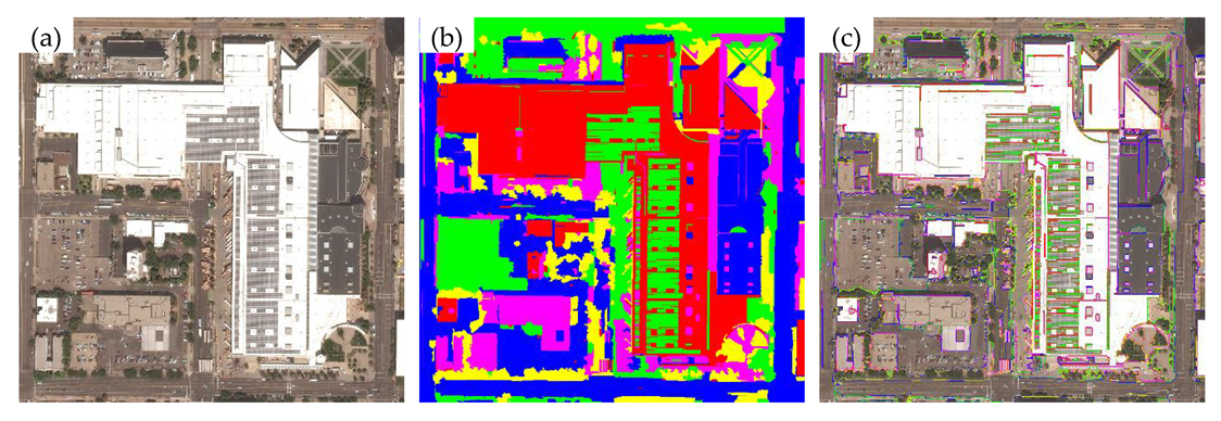
3.2. Performance Analysis

A Dell Power Edge R930 server with four sockets was used for the parallel performance analysis of the proposed parallel image segmentation method. The server had four Intel Xeon E7–8880 v3 @2.3GHz CPU, and each CPU had 18 cores (72 cores in total), 96 GB, 2133 MT/s memory, and a Samsung EVO Pro 512 GB SSD used as the operating system disk. The parallel computing toolbox of Matlab2018a software running on the Windows 10 operating system was used to implement the proposed method, which provided a parallel way through a multiworker mode.

In order to verify the parallel performance of the proposed parallel image segmentation method, two WorldView-3 Pan-Sharpened multiband images with 8192 × 8192 pixels/0.5-m spatial resolution/urban area of Saltlake, USA, and 7680 × 7680 pixels/0.3-m spatial resolution/Aeropueto de Madrid-Barajas Adolfo Suarez, Madrid, Spain, were used as experimental images (see Figure 18a,e), respectively. The segmentation parameters of the first experiments were set as same as those in Section 3.1, except the homogeneous regions K = 6 and the block tessellation scale 512 × 512. The segmentation parameters of second experiments were set as same as those in Section 3.1, except the homogeneous regions K = 6, the block tessellation scale was 512 × 512, the dividing scale S = 2000, the weight of spectral measure similarity α = 0.7, and the weight of region shape compactness γ = 0.4. In addition, considering the main land cover type was bare land, which had high heterogeneity in second experiment image (Figure 18e), the parameters (S, α, γ) of first experiment were different than the second experiment. S and γ were increased and α was decreased to improve the performance of the noice immunity of the parallel MHR method.

The experimental results are shown in Figure 18. The magnified areas highlighted in red and black boxes in Figure 18a,e are presented in Figure 18i,q (the images of Utah state office buildings and Salt Palace Convention Center) and Figure 18m,u (the images of airport terminal and parking lot), respectively. Figure 18b–d,f–h show the results of the segmentation outlines overlaid on the image, respectively. Figure 18j–l,n–p are the optimal segmentation results, respectively, while Figure 18r–t,v–x are the optimal segmentation outlines overlaid on the image, respectively. The findings suggest that visually, the results obtained by parallel MHR partitioning were relatively good, and the segmentation of complex object boundaries were complete and accurate.

In order to quantitatively evaluate the performance of the proposed parallel segmentation method, the runtime and speedup of the parallel MHR partitioning method, the parallel RHMRF-FCM segmentation method, and the proposed method were compared using different core numbers and segmentation parameters.

The runtime of the parallel MHR partitioning technique was tested using 8, 16, 24, 32, 40, 48, 56, and 64 cores. The results, as illustrated in Figure 19 by a blue curve, show the running time decreased rapidly with the increasing core number until it reached 48. At such point, the runtime became stable. This indicates that the best core number option for this experiment was 48. The speedup in the parallel MHR segmentation method is shown by the red curve in Figure 19. The results show that speedup increased rapidly as the core number increased until it reached 48, wherein the speedup tended to stabilize. The serial runtime of the minimum heterogeneous segmentation of an image with 8192 × 8192 pixels was then estimated by quadratic fitting. The runtime values for 128 × 128, 256 × 256, 512 × 512, 1024 × 1024, and 2048 × 2048 pixel images were used (see Figure 20a). The fitting function and fitting results are presented in Equation (40) and Figure 20b, respectively.

$$\mathit{f}\left(\mathit{N}\right)=4.59\times {10}^{-10}{\mathit{N}}^2+0.02\mathit{N}-1.04\times {10}^4$$

(40)

where N is the pixel number of the test image. The speedup values may have been overestimated in these experiments. On the one hand, using the theoretical analysis, the serial running time of the 8192 × 8192 pixel image was estimated using the fitting function, which may have resulted in significant deviations from the actual runtime. On the other hand, the time complexity of the serial algorithm in the proposed method was high given that the algorithm uses the MST model, and the calculation efficiency when implementing the model may not have been optimal. However, the speedup curve can also roughly reflect the proposed parallel MHR partitioning method, which had a significantly parallel performance.

The runtime of the parallel RHMRF-FCM segmentation method was tested using 1, 2, 4, 8, 16, 24, 32, 40, 48, 56, and 64 cores. The results, presented in a blue curve in Figure 20, show that runtime decreased rapidly with the increasing core number until the core number reached 16, and then the runtime tended to stabilize. When the core number was at 56, the runtime was minimum, which was only 24% of the serial algorithm, and the acceleration effect was significant. Therefore, for the parallel computing environment, using 56 cores for block parallel partitioning was the optimal choice, while 16 was the choice with the high-cost performance. The speedup of the parallel RHMRF-FCM segmentation method is shown by the red curve in Figure 21. As the number of cores increased, the speedup increased rapidly, until the core number reached 16. At such point, the speedup was at 3.5 and became stable, and the effect of parallel acceleration was also significant. In terms of the magnitude of speedup, the parallel optimal segmentation method was two orders lower than the parallel MHR segmentation technique. This is because the serial RHMRF-FCM algorithm was affected by its iterative solution method, and it was difficult to achieve large-scale performance improvements through parallel computing.

Figure 22 shows the runtime (in a blue curve) and speedup (in a red curve) of the proposed parallel segmentation method. The overall trend of the curves shows distinct similarities with the results of the MHR segmentation (Figure 19). With increasing the core number, the runtime and the speedup rapidly decreased and increased, respectively. After 48 cores, the curves tended to stabilize. The best parallel performance was achieved at 56 cores, with a runtime of 3685 s (about 1 h).

3.3. Discussion

In the parallel cost analysis experiment, we qualitatively and quantitatively evaluated the influence of different block tessellation scale on the final segmentation results. The results suggest the following conclusions: (a) With the increasing block tessellation scale, the similarity increased between the parallel segmentation results and serial segmentation results in terms of visual examination and quantitative accuracy evaluation results. This demonstrates the effectiveness of the proposed parallel MHR partitioning method. (b) For a WorldView-3 remote sensing image with 0.5-m resolution, the most reasonable block tessellation scale was 512 × 512. Using such setting, the accuracy loss in segmentation was constrained within 2% compared with the control group, which is generally acceptable in most applications. In the parallel performance analysis experiment, relatively good results were obtained using the parallel MHR partitioning method. The segmentation results of complex object boundaries were found to be complete and accurate. For a WorldView-3 Pan-Sharpened multiband remote sensing image with 8192 × 8192 pixels and 0.5-m spatial resolution, the running time and speedup curve for the parallel MHR partitioning, parallel RHMRF-FCM, and the proposed method were examined using four sockets server with 72 Cores. The results demonstrate that the proposed method has a high parallel performance.

4. Conclusions

High-resolution imagery offers rich geometric, texture, and spectral information, and is characterized by big data. These features bring new challenges to traditional image segmentation methods. To this end, this study proposed an efficient parallel high-resolution image segmentation method based on the MST and RHMRF-FCM model. There are two main contributions of this research: (a) On the basis of image domain decomposition by regular tessellation, block partitioning was executed in parallel by the MHR technique and integrated with the block IMSTF model, which effectively expressed the image’s explicit and implicit features. The parallel block merging method was then proposed to decrease the impact of landscape caused by image tessellation. (b) A parallel RHMRF-FCM segmentation method based on master-slave parallel mode was proposed to improve the computing performance of the serial RHMRF-FCM method, which effectively decreased the amount of data synchronization in parallel algorithms.

The proposed method has the following advantages: (a) By introducing the shape proportionality expressed on the IMSTF model, it serves as a much improved version of the MHR technique that is able to solve the problems of geometric noise and increased heterogeneity in homogeneous regions of high-resolution images. (b) The new method provides an efficient segmentation framework for big-scale high-resolution images using a parallel MHR partitioning technique, a parallel merging method based on image tessellation, and a parallel RHMRF-FCM segmentation method with low data synchronization traffic parallel scheme.

Further research can focus on the following directions: (a) Other parallel partitioning methods for big-scale high-resolution images can be explored through the creation of a more effective coordination mechanism between blocks. (b) Also, the proposed method can be applied to examine different types of remote sensing data, such as hyperspectral image and SAR image, and other applications, such as feature extraction and target identification.

References

1. Jensen, J. Introductory Digital Image Processing: A Remote Sensing Perspective, 3rd ed.; Prentice Hall: Upper Saddle River, NJ, USA, 2005. [Google Scholar]
2. Zhao, X.; Li, Y.; Zhao, Q. Mahalanobis distance based on fuzzy clustering algorithm for image segmentation. Digit. Signal Process. 2015, 43, 8–16. [Google Scholar] [CrossRef]
3. Li, Y. Remotely Sensed Data Segmentation under a Spatial Statistics Framework. Ph.D. Thesis, University of Waterloo, Waterloo, Ontario, 2009. [Google Scholar]
4. Curran, P. Remote sensing: Using the spatial domain. Environ. Ecol. Stat. 2001, 8, 331–344. [Google Scholar] [CrossRef]
5. Wang, C.; Xu, A.; Li, X. Supervised classification high-resolution remote-sensing image based on interval type-2 fuzzy membership function. Remote Sens. 2018, 10, 710. [Google Scholar] [CrossRef] [Green Version]
6. Li, D.; Tong, Q.; Li, R.; Gong, J.Y.; Zhnag, L. Current issues in high-resolution earth observation technology. Sci. China Earth Sci. 2012, 55, 1043–1051. (In Chinese) [Google Scholar] [CrossRef]
7. Benediktsson, J.; Chanussot, J.; Moon, W. Very high-resolution remote sensing: Challenges and opportunities. Proc. IEEE 2012, 100, 1907–1910. [Google Scholar] [CrossRef]
8. Ma, Y.; Wu, H.; Wang, L.; Huang, B.; Rangjan, R.; Zomaya, A.; Jie, W. Remote sensing big data computing: Challenges and opportunities. Future Gener. Comput. Syst. 2015, 51, 47–60. [Google Scholar] [CrossRef]
9. Rathore, M.; Paul, A.; Ahmad, A.; Chen, B.W.; Huang, B.; Ji, W. Real-time big data analytical architecture for remote sensing application. IEEE J. Sel. Top. Appl. Earth Obs. Remote Sens. 2015, 8, 4610–4621. [Google Scholar] [CrossRef]
10. Lin, W.; Li, Y.; Zhao, Q. High-resolution remote sensing image segmentation using minimum spanning tree tessellation and RHMRF-FCM algorithm. Acta Geod. Cartogr. Sin. 2019, 48, 64–74. (In Chinese) [Google Scholar]
11. Dearo, G.; Coelho, N. Multiple parallel mapreduce k-means clustering with validation and selection. In Proceedings of the 2014 Brazilian Conference on Intelligent Systems, IEEE Computer Society, Sao Paulo, Brazil, 18–22 October 2014; pp. 432–437. [Google Scholar]
12. Gu, H.; Han, Y.; Yang, Y.; Li, H.; Liu, Z.; Soergel, U.; Blaschke, T.; Cui, S. An efficient parallel multi-scale segmentation method for remote sensing imagery. Remote Sens. 2018, 10, 590. [Google Scholar] [CrossRef] [Green Version]
13. Du, Z.; Gu, Y.; Zhang, C.; Zhang, F.; Liu, R.; Sequeira, J.; Li, W. ParSymG: A parallel clustering approach for unsupervised classification of remotely sensed imagery. Int. J. Digit. Earth 2016, 1–19. [Google Scholar] [CrossRef]
14. Guan, Q.; Clarke, K. A general-purpose parallel raster processing programming library test application using a geographic cellular automata model. Int. J. Geogr. Inf. Sci. 2010, 24, 695–722. [Google Scholar] [CrossRef] [Green Version]
15. Xing, J.; Sieber, R.; Kalacska, M. The challenges of image segmentation in big remotely sensed imagery data. Ann. GIS 2014, 20, 233–244. [Google Scholar] [CrossRef]
16. Peng, B.; Zhang, L.; Zhang, D. A survey of graph theoretical approaches to image segmentation. Pattern Recognit. 2013, 46, 1020–1038. [Google Scholar] [CrossRef] [Green Version]
17. Geetha, M.; Rakendu, R. An improved method for segmentation of point cloud using minimum spanning tree. In Proceedings of the 2014 International Conference on Communications & Signal Processing, Melmaruvathur, India, 3–5 April 2014; pp. 833–837. [Google Scholar]
18. Sharifi, M.; Kiani, K.; Kheirkhahan, M. A Graph-Based Image Segmentation Approach for Image Classification and Its Application on SAR Images. Prz. Elektrotech. 2013, 89, 202–205. [Google Scholar]
19. Wu, Z.; Leahy, R. An optimal graph theoretic approach to data clustering: Theory and its application to image segmentation. IEEE Trans. Pattern Anal. Mach. Intell. 1993, 15, 1101–1113. [Google Scholar] [CrossRef] [Green Version]
20. Banerjee, B.; Varma, S.; Buddhiraju, K.; Eeti, L.N. Unsupervised multi-spectral satellite image segmentation combining modified mean-shift and a new minimum spanning tree based clustering technique. IEEE J. Sel. Top. Appl. Earth Obs. Remote Sens. 2014, 7, 888–894. [Google Scholar] [CrossRef]
21. Cui, W.; Zhang, Y. An effective graph-based hierarchy image segmentation. Intell. Autom. Soft Comput. 2011, 17, 969–981. [Google Scholar] [CrossRef]
22. Baatz, M.; Schäpe, A. Multiresolution segmentaion: An optimization approach for high quality multi-scale image segmentation. In Angewandte Geographische Informationsverarbeitung XII; Strobl, J., Blaschke, T., Griesebner, G., Eds.; Wichmann: Heidelberg, Germany, 2000; pp. 12–23. [Google Scholar]
23. Judah, A.; Hu, B.X.; Wang, J.G. An Algorithm for Boundary Adjustment toward Multi-Scale AdaptiveSegmentation of Remotely Sensed Imagery. Remote Sens. 2014, 6, 3583–3610. [Google Scholar] [CrossRef] [Green Version]
24. Wang, P.; Wei, Z.; Cui, W.; Lin, Z. A image segmentation method based on statistics learning theory and minimum spanning tree. Geomat. Inf. Sci. Wuhan Univ. 2017, 42, 877–883. (In Chinese) [Google Scholar]
25. Zhao, Q.; Li, X.; Zhao, X.; Li, Y. Fuzzy ISODATA Image Segmentation Intergrating Voronoi Tessellation HMRF Model. J. Signal Process. 2016, 32, 1233–1243. [Google Scholar]
26. Zhao, Q.; Li, X.; Zhao, X.; Li, Y. Remote Sensing Image Segmentation Algorithm with Regional Fuzzy Cluster and Mahalanobis Distance. J. China Univ. Min. Technol. 2017, 46, 222–228. [Google Scholar]
27. Lucarini, V. Symmetry-Break in Voronoi Tessellations. Symmetry 2009, 1, 21–54. [Google Scholar] [CrossRef] [Green Version]
28. Schneider, R. Weighted faces of Poisson Hyperplane Tessellations. Adv. Appl. Probab. 2009, 41, 682–694. [Google Scholar] [CrossRef]
29. Wang, Y.; Li, Y.; Zhao, Q. SAR Image Segmentation Combined Regular Tessellation and M-H Algorithm. Geomat. Inf. Sci. Wuhan Univ. 2016, 41, 1491–1497. [Google Scholar]
30. Achanta, R.; Shaji, A.; Smith, K. SLIC Superpixels Compared to State-of-the-Art Superpixel Methods. IEEE Trans. Pattern Anal. Mach. Intell. 2012, 34, 2274–2282. [Google Scholar] [CrossRef] [PubMed] [Green Version]
31. Baatz, M.; Schäpe, A. An optimization approach for high quality multi-scale image segmentation. In Beiträge Zum AGIT-Symposium; Herber Wichmann-Verlag: Berlin, Germany, 2000; pp. 12–23. [Google Scholar]
32. Li, H.; Tang, Y.; Liu, Q.; Ding, H.; Jing, L. An improved algorithm based on minimum spanning tree for multi-scale segmentation of remote sensing imagery. Acta Geod. Cartogr. Sin. 2015, 44, 791–796. (In Chinese) [Google Scholar]
33. Zhao, Q.; Li, X.; Li, Y.; Zhao, X. A fuzzy clustering image segmentation algorithm based on Hidden Markov Random Field models and Voronoi Tessellation. Pattern Recognit. Lett. 2017, 85, 49–55. [Google Scholar] [CrossRef]
34. Cannon, R.L.; Dave, J.V.; Bezdek, J.C.; Trivedi, M.M. Segmentation of a thematic mapper image using the fuzzy c-means clustering algorithm. IEEE Trans. Geosci. Remote Sens. 1986, 24, 400–408. [Google Scholar] [CrossRef]
35. Miyamoto, S.; Ichihashi, H.; Honda, K. Algorithms for Fuzzy Clustering; Springer: Heidelberg, Germany, 2008. [Google Scholar]
36. Prim, R. Shortest connection networks and some generalizations. Bell Syst. Tech. J. 1957, 36, 1389–1401. [Google Scholar] [CrossRef]
37. Kruskal, J. On the shortest spanning subtree of a graph and the traveling salesman problem. Proc. Am. Math. Soc. 1956, 7, 48–50. [Google Scholar] [CrossRef]
38. Kruskal’s Minimum Spanning Tree Algorithm|Greedy Algo-2. Available online: https://www.geeksforgeeks.org/kruskals-minimum-spanning-tree-algorithm-greedy-algo-2/ (accessed on 20 January 2020).
39. Thomas, H.; Charles, E.; Ronald, L.; Clifford, S. Introduction to Algorithms, 3rd ed.; The MIT Press: Cambridge, MA, USA, 2009. [Google Scholar]
40. Chatzis, S.; Varvarigou, T. A fuzzy clustering approach toward hidden Markov random field models for enhanced spatially constrained image segmentation. IEEE Trans. Fuzzy Syst. 2008, 16, 1351–1361. [Google Scholar] [CrossRef]
41. Rosu, R.-G.; Giovannelli, J.-F.; Giremus, A.; Vacar, A. Potts model parameter estimation in Bayesian segmentation of piecewise constant images. In Proceedings of the 2015 IEEE International Conference on Acoustics, Speech and Signal Processing (ICASSP), IEEE, Brisbane, Australia, 19–24 April 2015; pp. 4080–4084. [Google Scholar]
42. Chen, W.; Ostrouchov, G.; Pugmire, D.; Prabhat, M.; Wehner, M.F. A parallel EM algorithm for model-based clustering applied to the exploration of large spatio-temporal data. Technometrics 2013, 55, 513–523. [Google Scholar] [CrossRef]
43. Trobec, R.; Slivnik, B.; Bulić, P.; Robic, B. Introduction to Parallel Computing: From Algorithms to Programming on State-of-the-Art Platforms; Springer: Beilin, Germany, 2018. [Google Scholar]
44. Congalton, R.; Green, K. Assessing the Accuracy of Remotely Sensed Data: Principles and Practices; Lewis Publishers: Boca Raton, FL, USA, 1999. [Google Scholar]
Figure 1. Calculation method of adjacent edge set Et.
Remotesensing 12 00783 g001
Figure 2. The iteration procedure of the proposed image minimum spanning tree (MST) generation method based on the Kruskal algorithm. (a)–(y) show the variation of the tree marker vector t with each iteration.
Remotesensing 12 00783 g002
Figure 3. Procedure for the regional outer rectangular perimeter and regional outline. (a) shows the outer rectangular perimeter of a region, and (b,c) show the procedure of region outline.
Remotesensing 12 00783 g003
Figure 4. Procedure for merging two regions. (a) shows the regional outer rectangular perimeter bti and regional outline lti of region Fti; (b) shows the regional outer rectangular perimeter bti and regional outline lti of region Fti; (c) shows shows the regional outer rectangular perimeter bmerge and regional outline lmerge of merged region (FtiFti).
Remotesensing 12 00783 g004
Figure 5. Minimum heterogeneity rule (MHR) partitioning method. (a) is a simulated image, (b) is the MST of the simulated image, and (c) is the result of the MHR partitioning method of the simulated image.
Remotesensing 12 00783 g005
Figure 6. Parallel scheduling of the block MHR partitioning technique.
Remotesensing 12 00783 g006
Figure 7. Block neighbor relationship. (a) represents the interblock merge set of the block and its neighborhood blocks, and (b) represents the block basic association structure.
Remotesensing 12 00783 g007
Figure 8. Block merging. (a) shows three blocks (ytTr, yt and yt+Tr) without merging procedure; (b) shows the merged blocks (ytTr and yt) status; (c) shows the merged blocks (yt, and yt+Tr) status in which block yt is the merged result in (b).
Remotesensing 12 00783 g008
Figure 9. Flowchart of the blocks merging procedure.
Remotesensing 12 00783 g009
Figure 10. Decomposing of blocks merging dependency. (a) is the computational dependency diagram of merging operations between blocks, (b,c) is the decomposing of blocks merging dependency results by horizontally and vertically, respectively.
Remotesensing 12 00783 g010
Figure 11. The aggregated result of horizontal and vertical merging tasks. (ad) are the first and second horizontal merging task sets, the first and second vertical merging task sets, respectively.
Remotesensing 12 00783 g011
Figure 12. Horizontal first-level merging parallel scheduling schematic diagram.
Remotesensing 12 00783 g012
Figure 13. Runtime flowchart of the parallel RHMRF-FCM algorithm.
Remotesensing 12 00783 g013
Figure 14. Experiment data and standard segmentation result. (a) is an experiment image, (b) is the standard segmentation result, and (c) is the experiment image superimposed with the regional boundaries of the standard segmentation result.
Remotesensing 12 00783 g014
Figure 15. Segmentation result by different tessellation scale.
Remotesensing 12 00783 g015
Figure 16. Comparison between the standard and control group segmentation results, (a,b) are the segmentation results of the standard and control group, respectively, (c,d) are the superposition image of the standard and control group, respectively.
Remotesensing 12 00783 g016
Figure 17. Spectral features distribution of III and IV homogeneous regions.
Remotesensing 12 00783 g017
Figure 18. Segmentation results of the whole scene images.
Remotesensing 12 00783 g018aRemotesensing 12 00783 g018b
Figure 19. Parallel block partitioning time and its speedup with different core numbers.
Remotesensing 12 00783 g019
Figure 20. Block partitioning time on different tessellation scale. (a) the running time curve of 128 × 128–2048 × 2048 pixel images; (b) the fitting running time curve of 128 × 128–8192 × 8192 pixel images.
Remotesensing 12 00783 g020
Figure 21. Runtime and speedup of parallel regionalization optimal segmentation method with different core numbers.
Remotesensing 12 00783 g021
Figure 22. Running time and speedup of the proposed method with different core numbers.
Remotesensing 12 00783 g022