Article

Remote Sensing Single-Image Resolution Improvement Using A Deep Gradient-Aware Network with Image-Specific Enhancement

1
School of Earth Sciences, Zhejiang University, Hangzhou 310027, China
2
Aix Marseille Univ, Université de Toulon, CNRS, LIS, Marseille 13001, France
*
Author to whom correspondence should be addressed.
Remote Sens. 2020, 12(5), 758; https://doi.org/10.3390/rs12050758
Submission received: 29 December 2019 / Revised: 21 February 2020 / Accepted: 21 February 2020 / Published: 26 February 2020

Abstract

:
Super-resolution (SR) is able to improve the spatial resolution of remote sensing images, which is critical for many practical applications such as fine urban monitoring. In this paper, a new single-image SR method, deep gradient-aware network with image-specific enhancement (DGANet-ISE) was proposed to improve the spatial resolution of remote sensing images. First, DGANet was proposed to model the complex relationship between low- and high-resolution images. A new gradient-aware loss was designed in the training phase to preserve more gradient details in super-resolved remote sensing images. Then, the ISE approach was proposed in the testing phase to further improve the SR performance. By using the specific features of each test image, ISE can further boost the generalization capability and adaptability of our method on inexperienced datasets. Finally, three datasets were used to verify the effectiveness of our method. The results indicate that DGANet-ISE outperforms the other 14 methods in the remote sensing image SR, and the cross-database test results demonstrate that our method exhibits satisfactory generalization performance in adapting to new data.

Graphical Abstract

1. Introduction

Remote sensing (RS) has become an indispensable technology for various applications, including agricultural survey, global surface monitoring, and climate change detection. However, owing to the limitations of RS devices, atmospheric disturbances, and other uncertain factors, it is hard to obtain images at the desired resolution [1]. Low-resolution RS images are gradually becoming an obstacle to many advanced tasks, such as finer-scale land cover classification [2], object recognition [3], and precise road extraction [4].
Super-resolution (SR) methods are devoted to improving image resolution beyond the acquisition equipment limits [5]. SR has the advantages of low cost, easy implementation, and high efficiency compared to updating image acquisition devices. Remote sensing super-resolution (RS-SR) approaches can be roughly divided into two categories: single-image SR (SISR) and multi-image SR (MISR). The former requires only one image of the target scene for generating high-resolution output [5], while the latter requires multiple images that differ in terms of their satellite, angles, and sensors. For example, the authors of [6] improved the spatial resolution of Landsat images by fusion with SPOT5 images; the authors of [7] fused the information of multi-angle images for super-resolution; the authors of [8,9] merged multispectral images with panchromatic images to generate images with high spatial and spectral resolutions. MISR usually requires the input of multiple low-resolution (LR) images of the same region, which are difficult to collect in practical applications. Additionally, the feature extraction and fusion process with various resolutions and sensors are time-consuming, which restricts the applications of these techniques in real scenarios. Therefore, SISR is typically used.
According to the evolutionary trend and the complexity of the methods, we roughly divided the SISR approaches into interpolation-based approaches and machine learning-based approaches. Additionally, as deep learning methods (which are part of machine learning methods) have boomed in recent years and have achieved great success in SISR, we separated deep learning-based methods from machine learning methods into a third category.
The main idea of interpolation-based SISR is to locate each pixel of an HR image to be restored in the corresponding LR images and to interpolate the pixel’s value accordingly [10]. Bicubic, bilinear, and nearest-neighbor interpolation approaches are commonly used, and some novel interpolation methods are available [11,12,13]. Interpolation-based approaches offer a simple and fast way to improve image resolution [14]. However, they restore the missing values from a local perspective; thus, the generated images usually lack detailed information.
Machine-learning-based approaches attempt to overcome the shortcomings of interpolation-based approaches by a data-driven mechanism. The neighbor embedding method [15], sparsity-based methods [16,17,18,19], local regression [20], self-similarity algorithm [21], anchored neighborhood regression [22,23], and naive Bayes [24] are effective machine learning SISR approaches. Accurate representation of image features is key to the success of machine learning methods [25]. However, the expression ability of handcrafted features in machine learning is limited; therefore, it is difficult to handle complex data with high quality and high resolution.
In recent years, deep learning-based methods have demonstrated their powerful nonlinear expression and deep feature extraction capabilities. [26] first introduced the convolutional neural network (CNN) to solve SISR tasks, which showed excellent performance. Subsequently, many CNN-based methods emerged, such as in [27,28,29]. Residual learning [25,28,30,31,32,33,34,35] has been proposed to relieve the difficulty of training deeper networks and to improve SR performance. Some models use prior information, such as edges [36] and segmentation probability maps [37], to improve the details and fidelity of the super-resolved images. Deep Laplacian pyramid networks (LapSRN) [38], EnhanceNet [39], and the enhanced deep residual network (EDSR) [40] have all achieved great success in SISR.
However, some challenges are encountered. First, preserving the geographic information such as terrain, structure, and edge details precisely is of great significance for RS-SR, as this information can strongly affect the accuracy of subsequent analysis. The image gradient, which can sensitively reflect the changes in small details of an image [41], is highly important for RS images, and many RS applications have utilized this image gradient information. For instance, [42] used the gradient map to represent the topographic surface, and [43] used the gradient map to extract object boundaries for satellite image classification.
Moreover, the available supervised learning methods perform much better when the test images and the training set are highly similar; however, if the test images differ substantially from the training set, the results may be strongly affected. Because RS images are acquired from different sensors, their spectral, temporal, and spatial resolutions are different. It is difficult to include all scenarios in the training set, which limits the practicality of the existing supervised models.
In view of the above problems, the deep gradient-aware network with the image-specific enhancement (DGANet-ISE) method is proposed to obtain higher resolution RS images. Specifically, an enhanced deep residual network is constructed to learn the relationship between low-resolution (LR) and high-resolution (HR) images. During the training phase, a new gradient-aware loss is proposed in this network to promote the extraction of more high-frequency information, and to generate HR images with more detail. Additionally, when faced with inexperienced images, the image-specific enhancement approach is designed in the test phase to further improve SR performance. Each test LR image is inputted into the DGANet to obtain a relevant super-resolved HR image. Then, the HR image is further improved via the ISE method. No additional information is needed in this module, which focused on the specific characteristics of the single image and on realizing adaptive enhancement. In summary, our contributions are fourfold:
(1)
A new SISR method, DGANet-ISE, which includes a deep gradient-aware network and an image-specific enhancement approach, is proposed to improve the spatial resolution of RS images.
(2)
A deep gradient-aware network is proposed to model the complex relationship between LR and HR images. A new gradient-aware loss is designed in the training process to preserve more image gradient information in the super-resolved RS images.
(3)
This paper proposes an image-specific enhancement approach to further improve the SISR performance of RS images and to enhance the generalization capability and the adaptability of our method when facing inexperienced images.
(4)
Three data sets are used for evaluating the performance of DGANet-ISE. Compared to 14 methods, the experimental results indicate the superiority of DGANet-ISE.z.

2. Materials and Methods

The objective of SISR is to construct an HR image from an LR image I L R . Representing the target HR image and the estimated image as I H R . and I H R , respectively, the more similar I H R . and I H R . are, the better the SR effect is. The images have C . color channels, and W is the width and H is the height of the images. t refers to the upscaling factor. In this section, a detailed description of the proposed method is presented. In addition, the evaluation criteria and comparison methods are introduced.

2.1. Overview of the Proposed Method

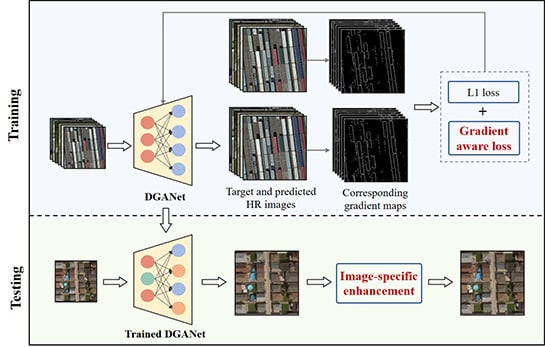
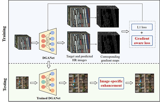
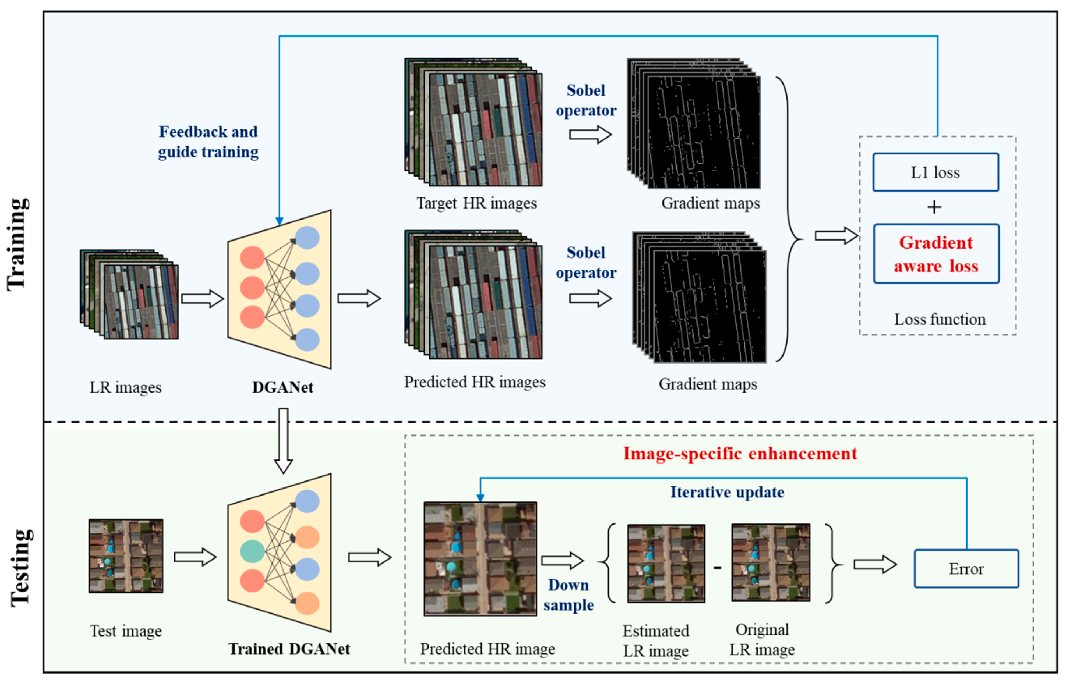
In this work, a new RS-SR method, DGANet-ISE, is proposed, as illustrated in Figure 1. The method mainly involves training and testing phases. The training phase aims at learning the complex relationships between LR and corresponding HR images. DGANet is the core element of this phase, and it is based on the enhanced residual network. This model employs residual and skip connections to devise a deep architecture, and it exhibits strong feature representation and nonlinear fitting abilities. As geographic information such as the terrain and edges are highly important for RS image interpretation, the precise preservation of more geographic details in the super-resolved images should be a focus of research. However, L 1 and L 2 losses generate blurry images in generation problems [44]. Therefore, we innovatively propose a new gradient-aware loss to alleviate this problem. Gradient-aware loss imposes gradient constraints to focus on the high-frequency signals in RS images, such as boundaries, edges, and terrains. As such, the proposed model can generate HR images with more detailed geographic information.
In the testing phase, the trained DGANet model is applied to generate primary HR results. However, if the testing images differ substantially from the training set (e.g., the images collected from different satellites), the performances of existing supervised learning methods will be strongly affected. To address this problem, an unsupervised learning-based enhancement approach, ISE, is introduced to further improve the performance and generate final HR images. ISE uses each input LR image to supplement more global information, and it has several advantages: (a) no additional supplementary data are required; (b) it focuses on the specific information and features of each test image, i.e., image-specific enhancement; (c) it boosts the generalization performance on inexperienced data sets.

2.2. Structure of DGANet

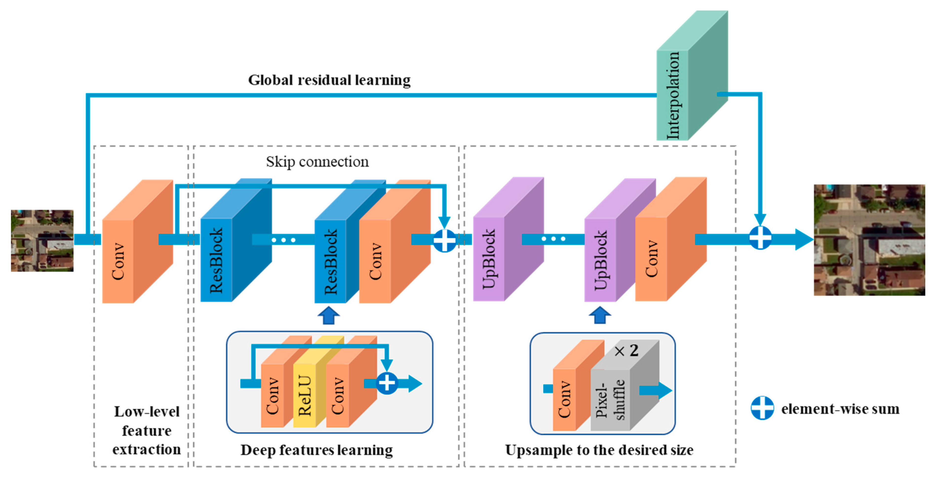
DGANet is proposed to extract the deep features of an LR image and upscale LR feature maps into HR output, as shown in Figure 2. The network contains different types of layers, including convolutional (Conv) layers, rectified linear unit (ReLU) layers, and pixel-shuffle layers. Based on these layers, residual blocks (ResBlocks) and upsample blocks (UpBlocks) are subsequently constructed. The ResBlocks are employed to construct deep networks, and UpBlocks to efficiently transform low-resolution feature maps into high-resolution size.
ResBlock: In each ResBlock, there are two Conv layers and one ReLU layer. The output is obtained by summing the input and the result obtained through the Conv and ReLU layers, as shown in Figure 2.
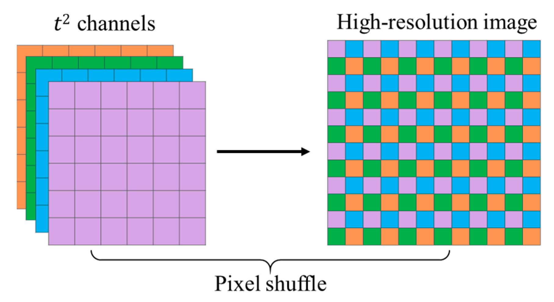
UpBlock: To transform the input feature maps to the target HR image, the UpBlocks are constructed based on one Conv layer and one pixel-shuffle layer. t represents the upscale factor. The Conv layer transforms the feature maps to t 2 channels and the pixel-shuffle layer is a periodic shuffling operator that rearranges the elements of a tensor   C × W × H × t 2 to a tensor of shape C × t W × t H (Figure 3). Each UpBlock upscales 2 times. Therefore, if the upscale factor is 2, one UpBlock is used; if the upscale factor is larger, multiple UpBlocks are used to improve the size gradually.
According to Figure 2, the whole network mainly consists of four modules: low-level features are extracted from the input image with Conv layers at the first module; the ResBlocks in the second module are used to learn more complex and deeper features; the third module transforms the feature maps from the LR domain to the HR domain; the last module is the global residual block, in which the input image is interpolated to high resolution directly to provide a large number of global signals of the input image.
Take an upscale factor of 8 as an example (the size of the input LR image is 32 × 32 ), Table 1 gives an exact representation of the components of DGANet. The kernel size of each Conv layer is 3 × 3 . Five ResBlocks are used to extract the deep features sufficiently in this network. For the global residual block, the bilinear interpolation algorithm is used to directly transform the input image to another image with the target resolution. In addition, the Adam optimizer was used to train the model, and the loss function will be introduced in the next section. The learning rate was 0.0001 and was halved every 40 epochs, and the batch size in the training phase was 32.

2.3. Gradient-Aware Loss

As images usually change quickly at the boundaries between objects, the image gradient is significant in boundary detection [41]. Therefore, the gradient information is usually used to extract object edges [43] and to reflect the changes in the surface’s topography [42] from RS images. L 1 and L 2 losses are widely used in deep learning applications, which are expressed below, where M is the number of samples of one batch. The batch size was 32 in this work.
L 1 = m = 1 M | I H R m I H R m | M
L 2 = m = 1 M ( I H R m I H R m ) 2 M
Although they can accurately represent the global pixel difference between images, they usually lead to smooth and blurred images [45], and little attention is paid to the important structure and edge information of RS images. Therefore, we propose a new gradient-aware loss ( L G a ) that facilitates the preservation of more edge and structure information and generates sharper HR images. The Sobel operator ( S o b ) [46] can effectively detect edges, and it enhances high spatial frequency details. Therefore, this operator is applied to generate gradient maps of the target image I H R and the predicted I H R images.
G M ( I H R ) = S o b ( I H R )
The gradient-aware loss is defined as the mean of M samples. The mean absolute error is used to evaluate the difference between gradient maps G M ( I H R ) and G M ( I H R ) , as shown below:
L G a = m = 1 M | G M ( I H R m ) G M ( I H R m ) | M
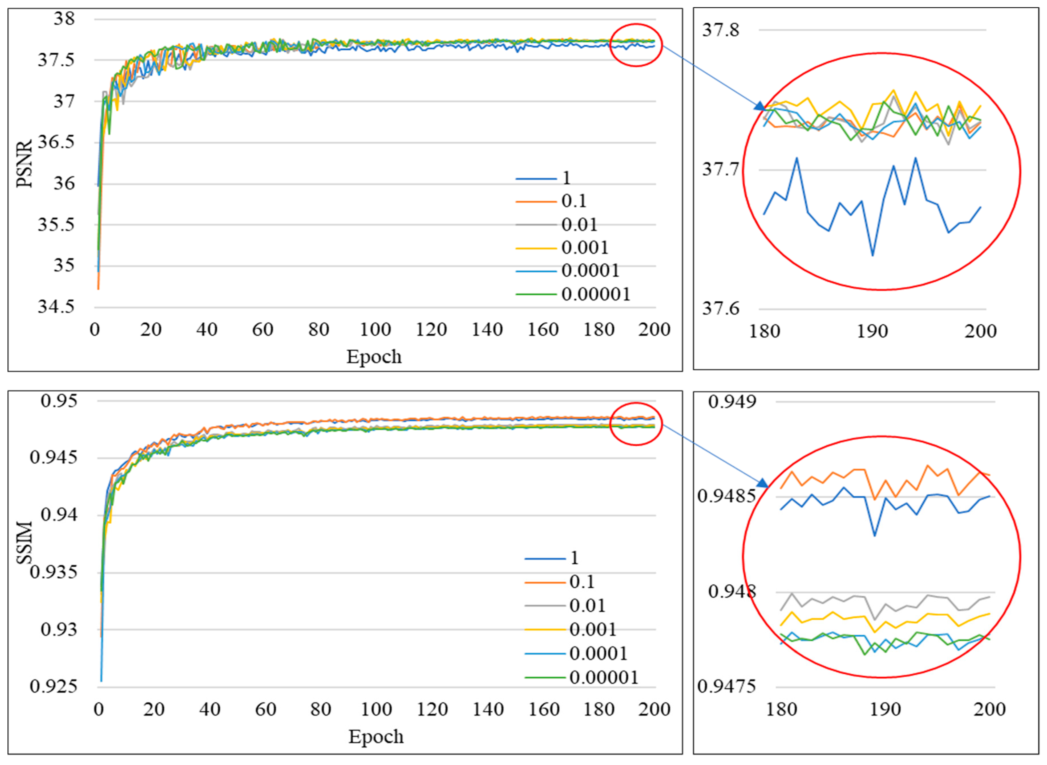
To maintain the balance between the global pixel error and the gradient error, a hyperparameter k is introduced. From the experiment, we found that k works best at 0.1 (as shown in Appendix A). Therefore,   k = 0.1 was used in this paper, and the overall loss function can be formulated as
L a l l = k × L G a + L 1
By using gradient-aware loss, more high-frequency information, such as edges and terrain, will be preserved in the super-resolution process, and sharper HR images with higher accuracy will be generated.

2.4. Image-Specific Enhancement

The performance of supervised methods largely depends on the training data set. If the test images differ substantially from the training set, the performance on inexperienced data will be greatly affected. As for RS images, they differ in terms of sensors, times, places, colors, types, and resolutions. It is hard to collect training samples that cover all scenarios, resulting in the insufficient generalization ability of many supervised SR methods. In this paper, the ISE algorithm is proposed to provide an effective solution to improve the generalization and adaptability of our method.
The core strategy of ISE is to back-project the error between the emulated and actual LR image to the SR image and to iteratively update it. This approach is inspired by the iterative back-projection algorithm (IBP) [47]. The specific procedure of ISE is presented in Algorithm 1, where the iteration number is n and N is the largest iteration number. The input of ISE is the original LR input I L R and the predicted HR image I H R obtained from the DGANet. The I H R is firstly downsampled to the LR domain ( I L R ). The difference image ( D i f f L ) between I L R and I L R is calculated. Then, the difference image is upsampled to the HR size, and subsequently, I H R can be updated by adding D i f f H to the predicted image. This process is repeated iteratively until the difference is sufficiently small or the N has been reached. The bilinear interpolation algorithm was used for upsampling and downsampling operations in this paper.
ISE is based on the assumption that if the estimated HR image is closer to the target image, the LR image I L R derived from the estimated HR image should be more similar to the input LR image. By backward-projecting the difference image between I L R and I L R to the super-resolved HR image, more differences can be considered in the estimated HR image. We can thereby obtain better SR results.
Algorithm 1. ISE
Input: LR input ( I L R ), predicted HR image ( I H R );
Output: Enhanced HR image ( I E H R );
While n < N or D i f f H is not sufficiently small
1. I L R = downsample ( I H R )
2. D i f f L = I L R I L R
3. D i f f H = u p s a m p l e ( D i f f L )
4. I H R = I H R +   D i f f H
5. n = n + 1
I E H R =   I H R
Return I E H R
The main advantages of ISE include that it requires no additional images for training. Furthermore, as ISE focuses on the characteristics of every single image, the image-specific information is used to further improve the quality of the super-resolved HR image. This way, the limitations that are due to the training data set can be effectively alleviated.

2.5. Evaluation Criteria and Baselines

2.5.1. Evaluation Criteria

The mean squared error (MSE), peak signal-to-noise ratio (PSNR) [48], and structural similarity index (SSIM) [49] are used to evaluate the performance of models, which are expressed as follows:
M S E = i = 1 t W j = 1 t H ( X i , j X ^ i , j ) 2 t 2 W H
P S N R = 20 × l o g 10 MAX R M S E ( X , X ^ )
S S I M = ( 2 μ X μ X ^ + c 1 ) × ( 2 σ X X ^ + c 2 ) ( μ X 2 + μ X ^ 2 + c 1 ) × ( σ X 2 + σ X ^ 2 + c 2 )
where X is the target high-resolution image; X ^ is the super-resolved image which is generated from the low-resolution image; tW and tH are the width and the height of the HR image, respectively; M A X represents the maximum pixel value in the original X image; R M S E is the root mean squared error; μ X and μ X ^ are the average pixel values of X and X ^ , respectively; σ X and σ X ^ are the variances of X and X ^ , respectively; and   σ X X ^ is the covariance of X and X ^ . Moreover,   c 1 = ( k 1 L ) 2 ,   c 2 = ( k 2 L ) 2 , where both variables are used to stabilize division with a weak denominator, and L is the dynamic range of the pixel values. The default values of k 1 and k 2 are k 1 = 0.01 and k 2 = 0.03 . M S E is commonly used to measure the error of super-resolved images. An M S E that is closer to 0 implies a higher model accuracy. P S N R is measured in decibels (dB).   S S I M is used to measure the similarity between two images [5]; the larger the value of P S N R and SSIM, the better the SR performance.

2.5.2. Methods to be Compared

Fourteen widely used SISR methods, which are shown in Table 2, were compared with DGANet-ISE. These SR methods use LR input images with three channels to generate super-resolved images. The input and output schemes were the same as proposed DGANet-ISE. The theory and characteristics of these methods were described in the corresponding references shown in Table 2.

3. Results

In this section, the data sets and the implementation details are introduced firstly. Subsequently, the performance of DGANet-ISE is verified by comparison with 14 different SR methods, and cross-database tests are performed to evaluate the generalization ability of our method.

3.1. Data Sets and Implementation Details

3.1.1. Data Sets

Three different data sets were employed to verify the effectiveness and superiority of DGANet-ISE.
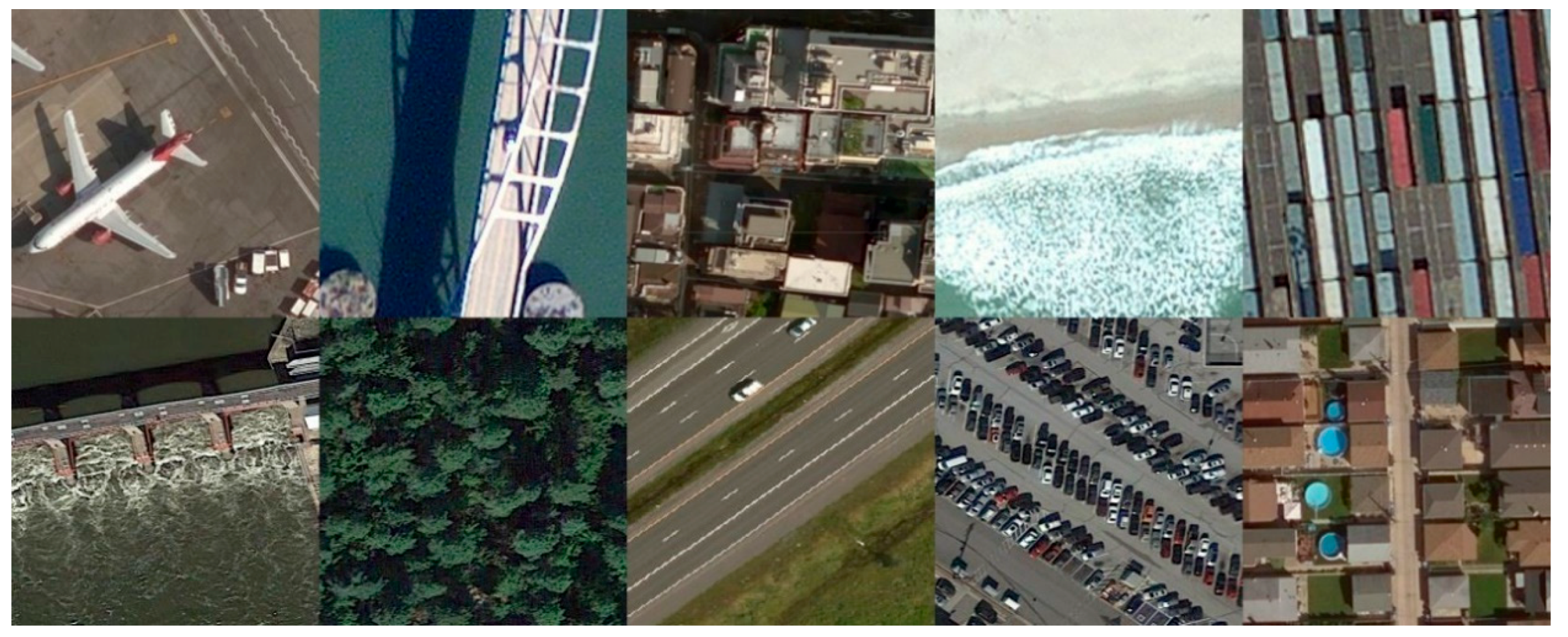
RSI-CB256 [55] contains 35 categories and about 24,000 images, which were collected for scene classification. This data set is rather challenging as the scenes are widely different. The pixel size of the images is 256 × 256 with 0.3–3 m spatial resolutions. Figure 4 shows the samples for 10 categories in the RSI-CB256 data set.
UCMerced [56] consists of 21 classes of land use images, including agricultural, airplane, beach, buildings, etc. Each class has 100 images with 256 × 256 pixels, and the spatial resolution is 1 foot ( 0.3 m).
Landsat-test is widely used, and the super-resolution of these images is of great value for many applications, such as finer land cover monitoring. The test images used in this paper were Landsat 5 TM data of band 7 (2.08–2.35 µm), band 4 (0.76–0.90 µm), and band 2 (0.52–0.60 µm). The data set was downloaded from the Google Earth Engine (https://developers.google.com/earth-engine/datasets/catalog/LANDSAT_LT05_C01_T1). The spatial resolution is 30 m. During the experiment, we cut the image into approximately 400 small images of 256 × 256 pixels. This data set is different from the RSI-CB256 and UCMerced data sets in two aspects: (1) the resolution of the Landsat data set is much smaller than the other two data sets, resulting in very different geographic information and scene content in the same image size; (2) the first two data sets are artificially selected into categories, while Landsat-test data set is a real unselected scene.

3.1.2. Implementation Details

As there are not enough corresponding LR–HR image pairs in reality, we downsampled the images using the Bicubic interpolation (BCI) algorithm with a factor of t { 2 , 4 ,   8 } to obtain LR images of different scales. Many studies, such as [29,35], have used BCI to generate LR–HR image pairs. The RSI-CB256 data set was used to compare our model with commonly used SISR methods, and all images were randomly divided into training samples (80%) and test samples (20%). Furthermore, in order to evaluate the generalization ability of our model, the Landsat-test data set was utilized for a cross-database test. That is, the models trained on RSI-CB256 were directly applied to the SR experiments of Landsat-test without any tuning. This is difficult because the data were collected from different sensors and have different spatial resolutions.
In addition, the UCMerced data set was randomly split into two balanced halves for training and testing, according to [35], which is consistent with other RS-SR methods, including CNN-7 [25], LGCNet [25], DCM [29], etc. Therefore, we compared our method with these RS-SR methods using the UCMerced data set.
The interpolation-based and deep learning-based methods were implemented in Python, and the machine learning-based methods were implemented in MATLAB. In addition, the models were used with the default settings suggested by the authors. The generation of LR images and the calculation of the evaluation criteria were implemented in the same Python environment to ensure the consistency and accuracy of the results.

3.2. Comparison with Baselines

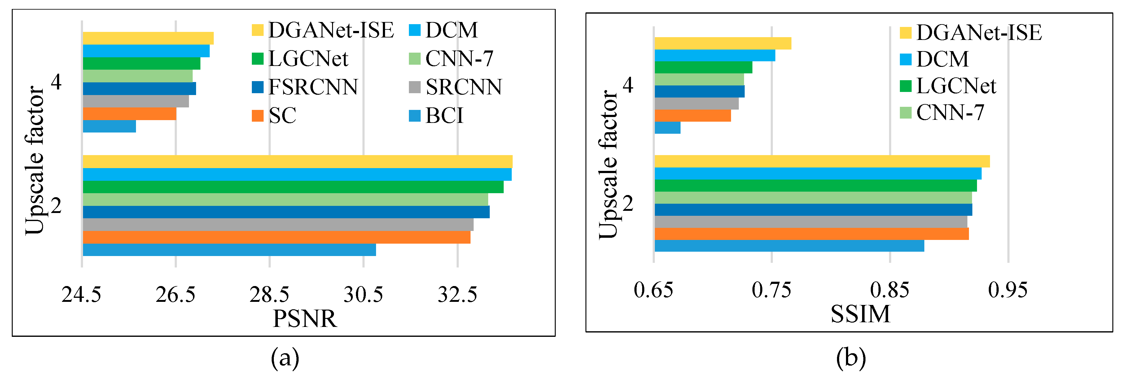
In this section, we experimented on the RSI-CB256 and UCMerced data sets, respectively. UCMerced is widely used in RS-SR; therefore, we compared our methods with the following RS-SR methods available in the literature [29], which experimented on the UCMerced data set as well. The upscale factors were 2 and 4, and the PSNR and SSIM results are shown in Table 3. In addition, Figure 5 provides a more vivid presentation of the comparison of the PSNR and SSIM results.
According to the table, compared with recent RS-SR methods, DGANet-ISE yields the best results. Although the PSNR values of our method and DCM are close, our SSIM results are larger than those of all of the compared approaches. The experimental results indicate that our method is good at structure reconstruction of RS images.
Additionally, another experiment was conducted on the RSI-CB256 data set, and DGANet-ISE was compared with three kinds of SISR methods: interpolation-based methods (nearest-neighbor interpolation (NNI), bilinear interpolation (BLI), and BCI), machine learning-based methods (simple functions (SF), neighbor embedding (NE), and classical sparsity-based super-resolution (SCSR)), and deep learning-based methods (super-resolution convolutional neural network (SRCNN), efficient sub-pixel convolutional network (ESPCN), and enhanced deep super-resolution network (EDSR)). The experiments were conducted with three different upscale factors, i.e., t { 2 ,   4 ,   8 } . The detailed results are presented in 
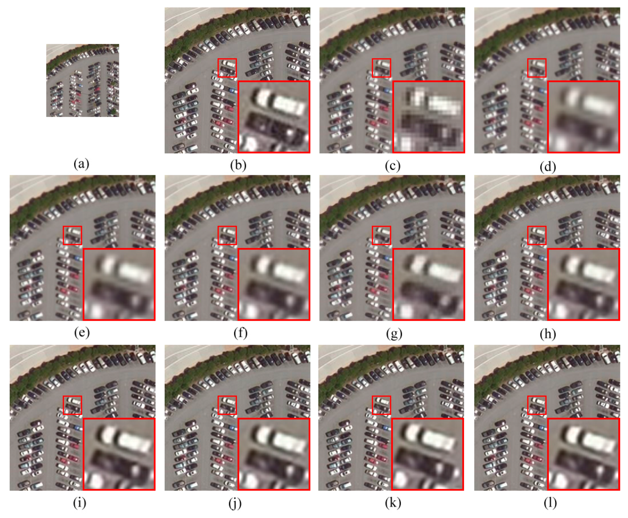
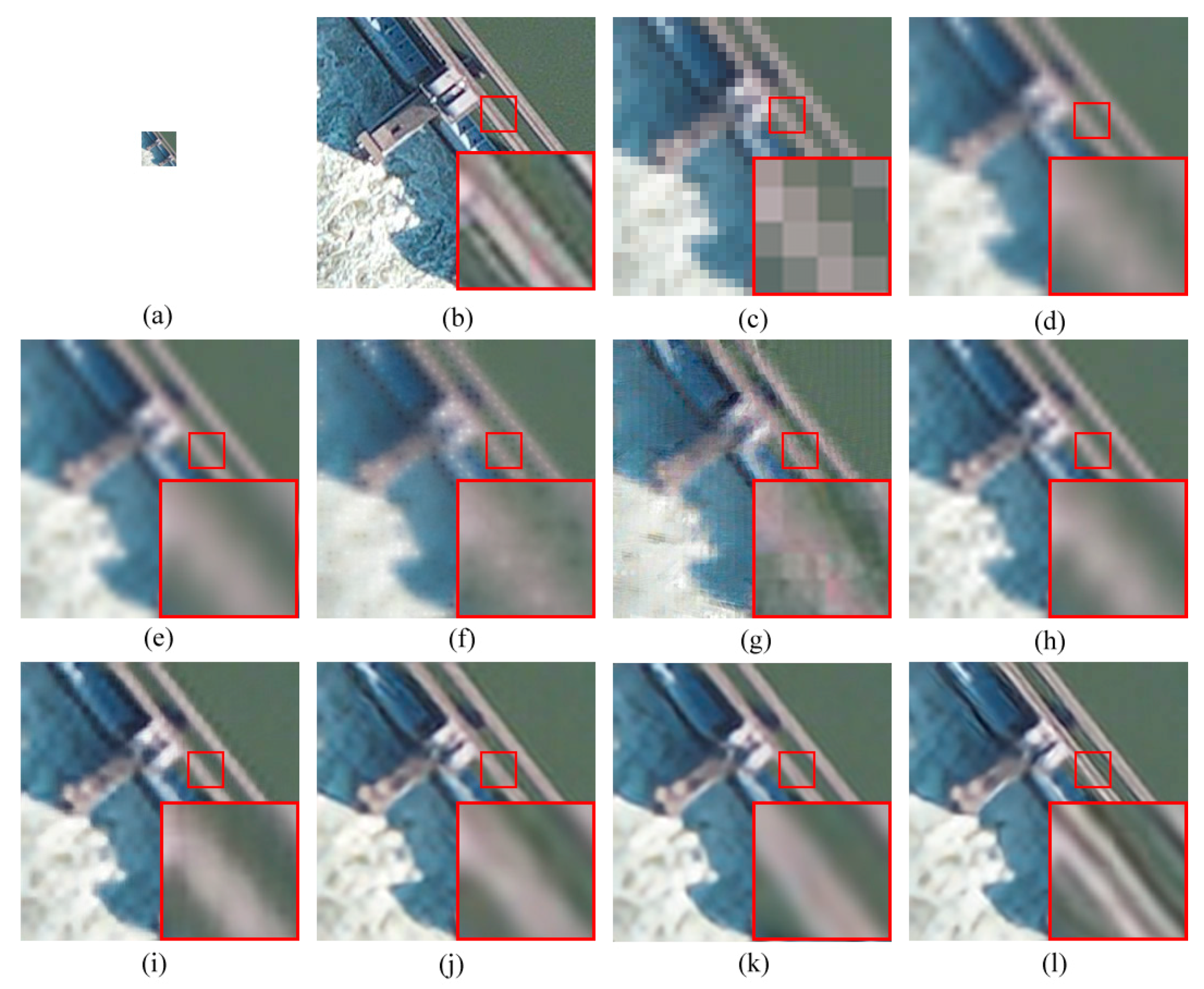
Table 4. In addition to the quantitative assessments, visual results are provided for a qualitative and intuitive evaluation. Three test images of a parking lot, a residence, and a dam were chosen as examples, and Figure 6, Figure 7 and Figure 8 show the super-resolved HR images for t { 2 ,   4 ,   8 } , respectively.
From the global perspective, it is obvious that as the upscale factor increases, the accuracy gradually decreases, because achieving super-resolution from a lower resolution image is much more difficult. Furthermore, according to Table 4, DGANet-ISE significantly outperforms the baselines. With the exception of DGANet-ISE, the results of EDSR are the best among the other methods. The PSNR values of DGANet-ISE are 0.33 dB, 0.26 dB, and 0.18 dB larger than those of EDSR when t is 2, 4, and 8, respectively.
BCI, SCSR, and DGANet-ISE are the most prominent within the interpolation, machine-learning, and deep learning categories, respectively. For example, when t = 2, the MSE values of BCI and SCSR are 69.74 and 48.01, respectively, much smaller than the other methods of the same category. With regard to deep learning methods, our proposed model exhibits superior performance on the SISR task. The MSE and PSNR results of our method are the best among all of the methods. For instance, when t = 2, the error of our proposed method is the smallest (MSE = 31.26), while PSNR = 37.92 dB and SSIM = 0.9477 are the largest.
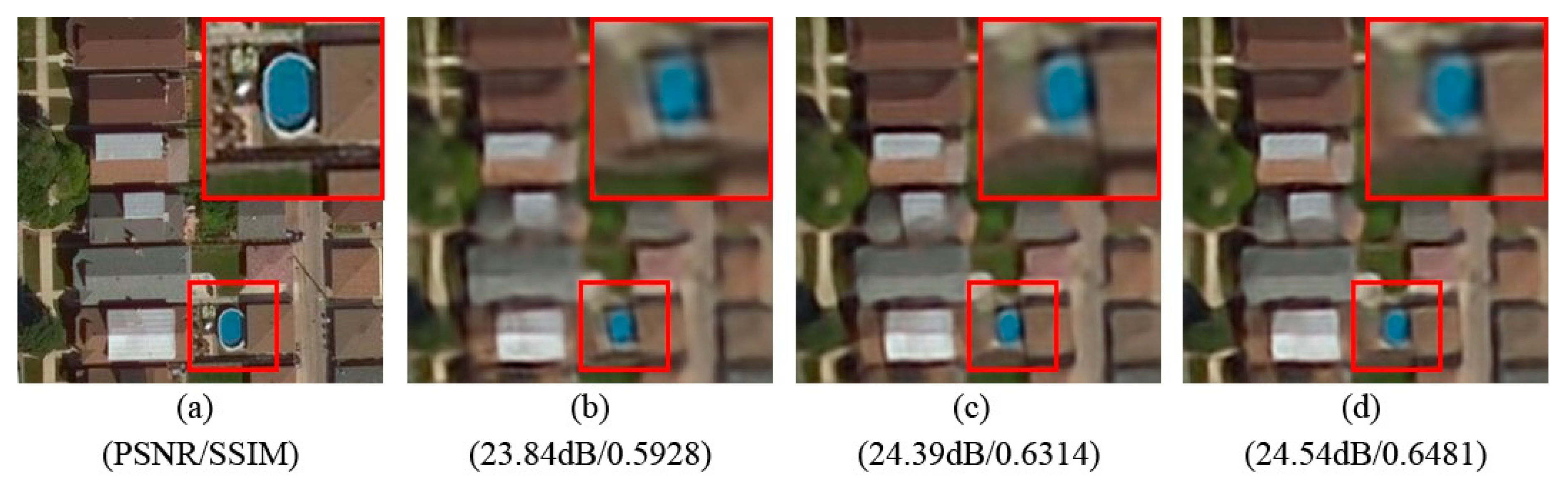
Focusing on the visual results (Figure 6, Figure 7 and Figure 8), the HR images super-resolved by different methods vary in terms of their features. For example, images obtained from NNI and NE have regular dense squares, similar to mosaics. This causes very blurred edges of these super-resolved images. The reason is that both algorithms rely heavily on the values of neighboring pixels or patches and ignore other significant structural details. NE performs better as it considers that the LR patches and the corresponding HR patches have similar local geometries.
In addition, images super-resolved via BLI and SCSR have very blurred boundaries (Figure 8d,h). We conducted a thorough analysis and found that both the BLI and SCSR algorithms use linear features for SISR, which results in the emergence of stripes when t increases. The basic idea of SCSR supposes that a signal can be represented as a sparse linear combination with respect to an overcomplete dictionary. A linear feature extraction operator behaves like a high-pass filter for feature representation of LR image patches [52]. In this way, the SCSR images have sharper edges than those of NE and BLI.
The HR images (Figure 7i–l) obtained by the deep learning methods generate smoother textures than the other two kinds of methods. DGANet-ISE yields more competitive visual results, because they are the most similar to their ground-truth HR counterparts. Our proposed DGANet-ISE recovers more texture and structure details, such as the edges of the dam in Figure 8. The edges of the dam generated by our method are very clear, whereas the edges are blurred or even missing in other images. This is because the gradient-aware loss proposed in our method can capture more gradient information of the RS images, which can facilitate the generation of sharper edges and textures. In summary, the proposed method performs the best compared to other methods.

3.3. Cross-Database Test

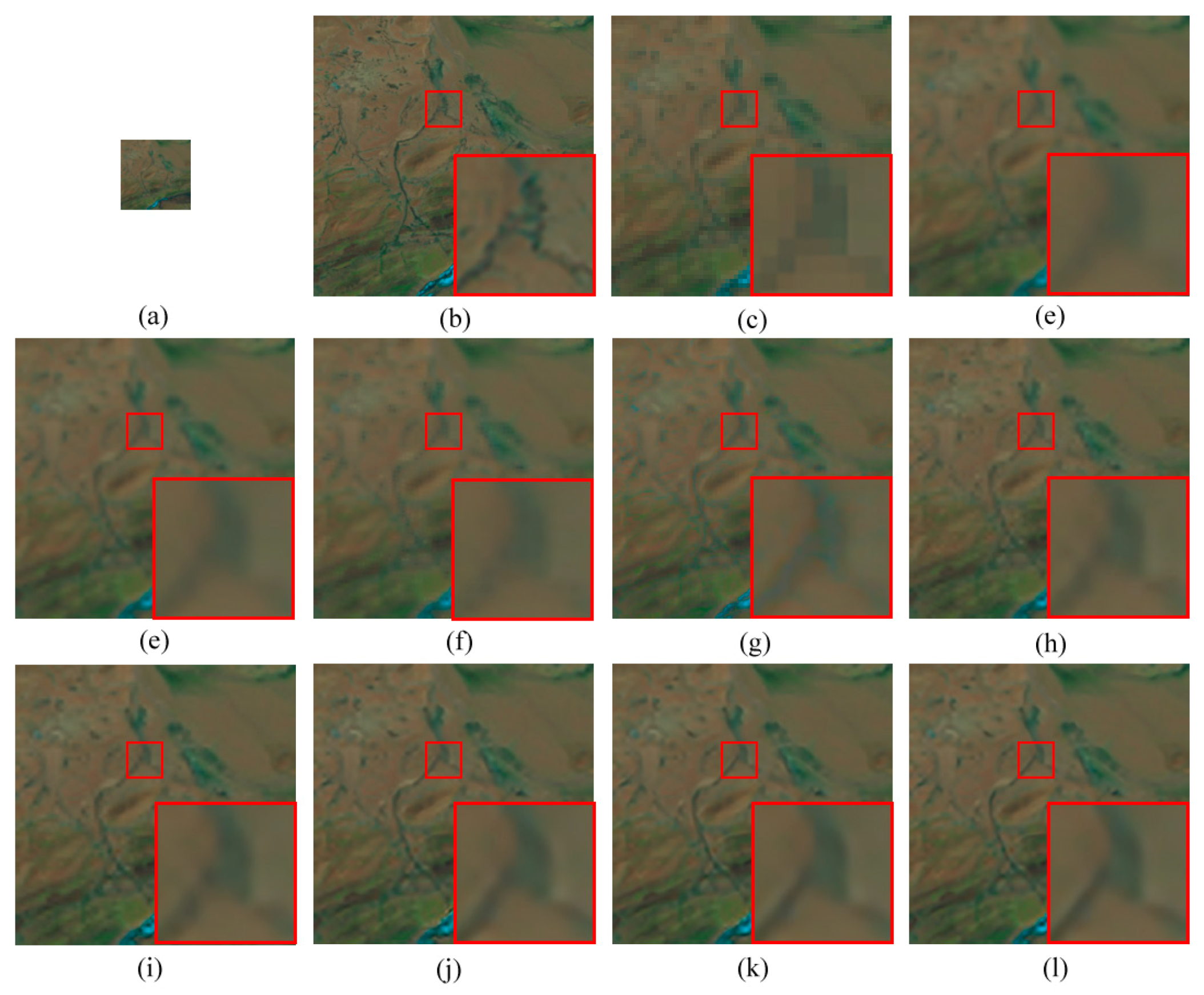
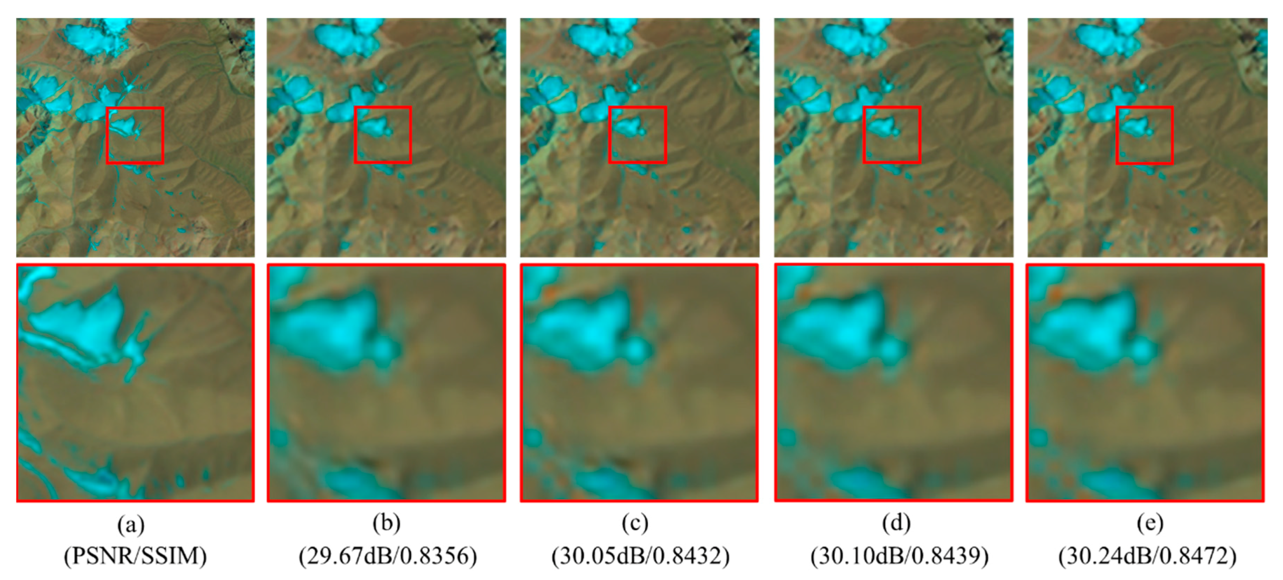
To further evaluate the robustness and generalization capability of DGANet-ISE, the Landsat-test data set was applied for a cross-database test, i.e., the models trained on the RSI-CB256 data set were directly used to super-resolve the Landsat-test data set without any fine-tuning or modification. The results of the comparison between the different approaches under the three upscale factors are presented in Table 5, and Figure 9 shows the visual results of the different methods on an example image.
The Landsat-test data set differs substantially from the training samples, since the spatial resolution of training samples is 0.3–3m, while the spatial resolution of Landsat-test images is 30 m, and the scene contents in the same image size are very different. Therefore, it poses a great challenge to apply these supervised learning models directly to such test images.
According to the results, our proposed method shows a reasonably satisfactory performance compared to the other methods. For instance, when t = 2, the PSNR is 40.70 dB, which is 0.64 dB larger than that of EDSR and 1.57 dB larger than that of SCSR. This is because the ISE algorithm focuses on the personalized features of each test image, and provides a fast additional improvement of the super-resolved HR image obtained from the deep gradient-aware network. In summary, DGANet-ISE has strong robustness and generalization capability on new data sets.

4. Discussion

In this section, ablation studies were conducted to analyze the performance of the proposed gradient-aware loss and the impact of the ISE algorithm.

4.1. Dependency on the Type of Loss Functions

For evaluating the effectiveness of gradient-aware loss, we trained the same network with the L 1 , L 2 , and gradient-aware losses on training samples of the RSI-CB256 data set. The detailed results on the test samples of the RSI-CB256 data set are presented in Table 6. As we can see, the PSNR results of L 1 loss are slightly better than those of the L 2 loss, and our proposed loss function yields the best results. When the upscale factor is 2, the PSNR obtained with the gradient-aware loss (37.92 dB) is 0.2 dB better compared to the L1 loss (37.72 dB) and the L2 loss (37.66 dB).
To assess the detailed information preservation capability of the gradient-aware loss, an image that belongs to the “Residence” class was selected for further analysis. Figure 10 presents the reconstructed HR images obtained using the three-loss functions with an upscale factor of 8. The PSNR result of the proposed loss is 25.54 dB, which is 0.15 dB larger than L1 loss. The shape and the direction of the swimming pool that is obtained with the gradient-aware loss are much closer to reality. In addition, the PSNR and SSIM results obtained by our gradient-aware loss are much better than L 1 and L 2 losses. In summary, our proposed gradient-aware loss is able to generate HR images more accurately.

4.2. Impact of ISE

Since ISE aims to improve the SR results of inexperienced data, in this part, cross-data set test performances of the method with and without ISE were compared. The DGANet and EDSR trained on the RSI-CB256 data set were directly applied to the Landsat-test data. The results are presented in Table 7 and Figure 11 gives a visual comparison. The results in Table 7 illustrate that the ISE approach can further improve the SR performance. For instance, when the upscale factor is 2, the PSNR of EDSR and DGANet is improved by 0.46 dB and 0.23 dB, respectively. By using the specific information of the test image, ISE can further enhance the HR results of DGANet. As ISE is an unsupervised approach, it can greatly improve the generalization and adaptivity of the models, and reduce the dependence on the training set.

5. Conclusions

A new SISR method, DGANet-ISE, was proposed in this work to increase the spatial resolution of RS images. Specifically, the deep gradient-aware network and image-specific enhancement are two important components of DGANet-ISE. The first part extracts features and learns the precise representation between the LR and HR domains. The gradient-aware loss was first proposed in this part to preserve the important gradient information of RS images. Image-specific enhancement was used to improve the robustness and adaptability of our method, thus further improving the performance. Based on the above, three different data sets were used as experimental data sets. The proposed DGANet-ISE was applied to super-resolve the RS images with three upscale factors, which yielded remarkable results. Compared to other SISR methods, DGANet-ISE is better from both quantitative and visual perspectives. Moreover, the results of the cross-database test demonstrate that the proposed approach exhibits strong generalization and robustness, and provides an excellent opportunity for practical applications.

Author Contributions

Conceptualization, M.Q. and Z.D.; methodology, M.Q.; validation, M.Q., L.H., and S.M.; supervision, Z.D., S.M., and J.S.; investigation, M.Q., L.H., S.M., and J.S.; writing—original draft preparation, M.Q.; writing—review and editing, M.Q.; project administration, Z.D., F.Z., and R.L.; resources, R.L.; funding acquisition, Z.D. All authors have read and agreed to the published version of the manuscript.

Funding

This research was supported by the National Key Research and Development Program of China under Grants 2016YFC1400903 and 2018YFB0505000, and the National Natural Science Foundation of China (41871287).

Acknowledgments

Thanks to all the anonymous reviewers for their constructive and valuable suggestions on the earlier drafts of this manuscript.

Conflicts of Interest

The authors declare no conflicts of interest.

Appendix A

To analyze the influence of the hyperparameter k value on the model, we plotted the trends of the average PSNR and SSIM values of k = { 1 , 0.1 ,   0.01 , 0.001 , 0.0001 , 0.00001 } versus the number of iterations (up to 200 epochs) in Figure A1. The experiment was conducted with an upscale factor of 2. When k = 1 , the PSNR is lower than other cases. In terms of the SSIM results, k = 1 and 0.1 performed better than the others. Therefore, in this paper, we used k = 0.1 as the final weight of the gradient-aware loss.
Figure A1. Comparison of peak signal-to-noise ratio (PSNR) and structural similarity index (SSIM) between the five different k values.
Remotesensing 12 00758 g0a1

References

  1. Yang, D.; Li, Z.; Xia, Y.; Chen, Z. Remote sensing image super-resolution: Challenges and approaches. In Proceedings of the 2015 IEEE International Conference on Digital Signal Processing (DSP), Singapore, 21–24 July 2015; pp. 196–200. [Google Scholar]
  2. Tatem, A.J.; Lewis, H.G.; Atkinson, P.M.; Nixon, M.S. Super-resolution land cover pattern prediction using a hopfield neural network. Remote Sens. Environ. 2002, 79, 1–14. [Google Scholar] [CrossRef] [Green Version]
  3. Cheng, G.; Han, J. A survey on object detection in optical remote sensing images. ISPRS J. Photogramm. Remote Sens. 2016, 117, 11–28. [Google Scholar] [CrossRef] [Green Version]
  4. Alshehhi, R.; Marpu, P.R.; Woon, W.L.; Mura, M.D. Simultaneous extraction of roads and buildings in remote sensing imagery with convolutional neural networks. ISPRS J. Photogramm. Remote Sens. 2017, 130, 139–149. [Google Scholar] [CrossRef]
  5. Haut, J.M.; Fernandez-Beltran, R.; Paoletti, M.E.; Plaza, J.; Plaza, A.; Pla, F. A new deep generative network for unsupervised remote sensing single-image super-resolution. IEEE Trans. Geosci. Remote Sens. 2018, 11, 6792–6810. [Google Scholar] [CrossRef]
  6. Song, H.; Huang, B.; Liu, Q.; Zhang, K. Improving the spatial resolution of Landsat TM/ETM+ through fusion with SPOT5 images via learning-based super-resolution. IEEE Trans. Geosci. Remote Sens. 2015, 53, 1195–1204. [Google Scholar] [CrossRef]
  7. Zhang, H.; Yang, Z.; Zhang, L.; Shen, H. Super-resolution reconstruction for multi-angle remote sensing images considering resolution differences. Remote Sens. 2014, 6, 637–657. [Google Scholar] [CrossRef] [Green Version]
  8. Lanaras, C.; Baltsavias, E.; Schindler, K. Hyperspectral super-resolution by coupled spectral unmixing. In Proceedings of the IEEE International Conference on Computer Vision, Las Condes, Chile, 11–18 December 2015; pp. 3586–3594. [Google Scholar]
  9. Yi, C.; Member, S.; Zhao, Y.; Chan, J.C. Hyperspectral image super-resolution based on spatial and spectral correlation fusion. IEEE Trans. Geosci. Remote Sens. 2018, 56, 4165–4177. [Google Scholar] [CrossRef]
  10. Xu, Z.; Wang, X.; Chen, Z.; Xiong, D.; Ding, M.; Hou, W. Nonlocal similarity based DEM super resolution. ISPRS J. Photogramm. Remote Sens. 2015, 110, 48–54. [Google Scholar] [CrossRef]
  11. Gunturk, B.K.; Glotzbach, J.; Altunbasak, Y.; Schafer, R.W.; Mersereau, R.M. Demosaicking: Color filter array interpolation. IEEE Signal Process. Mag. 2005, 22, 44–54. [Google Scholar] [CrossRef]
  12. Li, X.; Orchard, M.T. New edge-directed interpolation. IEEE Trans. Image Process. 2001, 10, 1521–1527. [Google Scholar]
  13. Zhang, L.; Wu, X. An edge-guided image interpolation algorithm via directional filtering and data fusion. IEEE Trans. Image Process. 2006, 15, 2226–2238. [Google Scholar] [CrossRef] [PubMed] [Green Version]
  14. Wu, W.; Yang, X.; Liu, K.; Liu, Y.; Yan, B.; Hua, H. A new framework for remote sensing image super-resolution: Sparse representation-based method by processing dictionaries with multi-type features. J. Syst. Archit. 2016, 64, 63–75. [Google Scholar] [CrossRef]
  15. Chang, H.; Yeung, D.; Xiong, Y.; Bay, C.W.; Kong, H. Super-resolution through neighbor embedding. In Proceedings of the 2004 IEEE Computer Society Conference on Computer Vision and Pattern Recognition, Washington, DC, USA, 27 June–2 July 2004; Volume 1, p. I-I. [Google Scholar]
  16. Peleg, T.; Elad, M. A statistical prediction model based on sparse representations for single image super-resolution. IEEE Trans. Image Process. 2014, 23, 2569–2582. [Google Scholar] [CrossRef] [PubMed]
  17. Dong, W.; Zhang, L.; Shi, G.; Wu, X. Image deblurring and super-resolution by adaptive sparse domain selection and adaptive regularization. IEEE Trans. Image Process. 2011, 20, 1838–1857. [Google Scholar] [CrossRef] [PubMed] [Green Version]
  18. Xinlei, W.; Naifeng, L. Super-resolution of remote sensing images via sparse structural manifold embedding. Neurocomputing 2016, 173, 1402–1411. [Google Scholar] [CrossRef]
  19. Tang, S.; Xu, Y.; Huang, L.; Sun, L. Hyperspectral Image Super-Resolution via Adaptive Dictionary Learning and Double l1 Constraint. Remote Sens. 2019, 11, 2809. [Google Scholar] [CrossRef] [Green Version]
  20. Gu, S.; Sang, N.; Ma, F. Fast image super resolution via local regression. In Proceedings of the 21st International Conference on Pattern Recognition (ICPR2012), Tsukuba, Japan, 11–15 November 2012; pp. 3128–3131. [Google Scholar]
  21. Pan, Z.; Yu, J.; Huang, H.; Hu, S.; Zhang, A.; Ma, H.; Sun, W. Super-resolution based on compressive sensing and structural self-similarity for remote sensing images. IEEE Trans. Geosci. Remote Sens. 2013, 51, 4864–4876. [Google Scholar] [CrossRef]
  22. Timofte, R.; De Smet, V.; Van Gool, L. Anchored neighborhood regression for fast example-based super-resolution. In Proceedings of the IEEE international conference on computer vision, Sydney, Australia, 1–8 December 2013; pp. 1920–1927. [Google Scholar]
  23. Timofte, R.; De Smet, V.; Van Gool, L. A+: Adjusted anchored neighborhood regression for fast super-resolution. In Asian Conference on Computer Vision; Springer: New York, NY, USA, 2014; pp. 111–126. [Google Scholar]
  24. Salvador, J.; Perez-Pellitero, E. Naive bayes super-resolution forest. In Proceedings of the IEEE International conference on computer vision, Santiago, Chile, 7–13 December 2015; pp. 325–333. [Google Scholar]
  25. Lei, S.; Shi, Z.; Zou, Z. Super-resolution for remote sensing images via local-global combined network. IEEE Geosci. Remote Sens. Lett. 2017, 14, 1243–1247. [Google Scholar] [CrossRef]
  26. Dong, C.; Loy, C.C.; He, K.; Tang, X. Learning a deep convolutional network for image super-resolution. In European Conference on Computer vision; Springer: New York, NY, USA, 2014; pp. 184–199. [Google Scholar]
  27. Ledig, C.; Theis, L.; Husz, F.; Caballero, J.; Cunningham, A.; Acosta, A.; Aitken, A.; Tejani, A.; Totz, J.; Wang, Z.; et al. Photo-realistic single image super-resolution using a generative adversarial network. Proc. IEEE Conf. Comput. Vis. Pattern Recognit. 2017, 2, 4681–4690. [Google Scholar]
  28. Kim, J.; Lee, J.K.; Lee, K.M. Accurate image super-resolution using very deep convolutional networks. In Proceedings of the IEEE conference on computer vision and pattern recognition, Las Vegas, NV, USA, 26 June–1 July 2016; pp. 1646–1654. [Google Scholar]
  29. Haut, J.M.; Paoletti, M.E.; Fernandez-Beltran, R.; Plaza, J.; Plaza, A.; Li, J. Remote sensing single-image superresolution based on a deep compendium model. IEEE Geosci. Remote Sens. Lett. 2019, 16, 1432–1436. [Google Scholar] [CrossRef]
  30. Zhang, Y.; Li, K.; Li, K.; Wang, L.; Zhong, B.; Fu, Y. Image super-resolution using very deep residual channel attention networks. In Proceedings of the European Conference on Computer Vision (ECCV), Munich, Germany, 8–14 September 2018; pp. 286–301. [Google Scholar]
  31. Tai, Y.; Yang, J.; Liu, X. Image super-resolution via deep recursive residual network. In Proceedings of the IEEE conference on computer vision and pattern recognition, Honolulu, HI, USA, 21–26 July 2017; pp. 3147–3155. [Google Scholar]
  32. Ma, W.; Pan, Z.; Guo, J.; Lei, B. Achieving super-resolution remote sensing images via the wavelet transform combined with the recursive Res-Net. IEEE Trans. Geosci. Remote Sens. 2019, 57, 3512–3527. [Google Scholar] [CrossRef]
  33. Gu, J.; Sun, X.; Zhang, Y.; Fu, K.; Wang, L. Deep residual squeeze and excitation network for remote sensing image super-resolution. Remote Sens. 2019, 11, 1817. [Google Scholar] [CrossRef] [Green Version]
  34. Lu, T.; Wang, J.; Zhang, Y.; Wang, Z.; Jiang, J. Satellite image super-resolution via multi-scale residual deep neural network. Remote Sens. 2019, 11, 1588. [Google Scholar] [CrossRef] [Green Version]
  35. Haut, J.M.; Fernandez-Beltran, R.; Paoletti, M.E.; Plaza, J.; Plaza, A. Remote sensing image superresolution using deep residual channel attention. IEEE Trans. Geosci. Remote Sens. 2019, 57, 9277–9289. [Google Scholar] [CrossRef]
  36. Yang, W.; Feng, J.; Yang, J.; Zhao, F.; Liu, J.; Member, S. Deep edge guided recurrent residual learning for image super-resolution. IEEE Trans. Image Process. 2017, 26, 5895–5907. [Google Scholar] [CrossRef]
  37. Wang, X.; Yu, K.; Dong, C.; Loy, C.C. Recovering realistic texture in image super-resolution by deep spatial feature transform. In Proceedings of the IEEE conference on computer vision and pattern recognition, Salt Lake City, UT, USA, 18–23 June 2018; pp. 606–615. [Google Scholar]
  38. Lai, W.; Ahuja, N.; Yang, M.; Tech, V. Deep laplacian pyramid networks for fast and accurate super-resolution. In Proceedings of the IEEE conference on computer vision and pattern recognition, Honolulu, HI, USA, 21–26 July 2017; pp. 624–632. [Google Scholar]
  39. Sch, B.; Hirsch, M. EnhanceNet: Single image super-resolution through automated texture synthesis. In Proceedings of the IEEE International Conference on Computer Vision, Venice, Italy, 22–29 October 2017; pp. 4491–4500. [Google Scholar]
  40. Lim, B.; Son, S.; Kim, H.; Nah, S.; Lee, K.M. Enhanced deep residual networks for single image super-resolution. Proc. IEEE Conf. Comput. Vis. Pattern Recognit. Work. 2017, 1, 136–144. [Google Scholar]
  41. Jacobs, D. Image Gradients. Available online: https://www.cs.umd.edu/~djacobs/CMSC426/ImageGradients.pdf (accessed on 3 September 2019).
  42. Zhang, G.; Jia, X.; Hu, J. Superpixel-based graphical model for remote sensing image mapping. IEEE Trans. Geosci. Remote Sens. 2015, 53, 5861–5871. [Google Scholar] [CrossRef]
  43. Borra, S.; Thanki, R.; Dey, N. Recurrent neural network to correct satellite image classification maps. SpringerBriefs Appl. Sci. Technol. 2019, 55, 53–81. [Google Scholar]
  44. Li, Z.; Hu, Y.; Zhang, M.; Xu, M.; He, R. Protecting your faces: Meshfaces generation and removal via high-order relation-preserving CycleGAN. 2018 International Conference on Biometrics (ICB); IEEE: Piscataway, NJ, USA, 2018; pp. 61–68. [Google Scholar]
  45. Huang, H.; He, R.; Sun, Z.; Tan, T. Wavelet-SRNet: A wavelet-based CNN for multi-scale face super resolution. In Proceedings of the IEEE International Conference on Computer Vision, Venice, Italy, 22–29 October 2017; pp. 1689–1697. [Google Scholar]
  46. Sobel, I. An Isotropic 3 × 3 Image Gradient Operator. Machine vision for three-dimensional scenes; Academic Press: Orlando, FL, USA, 1990; pp. 376–379. [Google Scholar]
  47. Irani, M.; Peleg, S. Improving resolution by image registration. CVGIP Graph. Model. image Process. 1991, 53, 231–239. [Google Scholar] [CrossRef]
  48. Huynh-Thu, Q.; Ghanbari, M. Scope of validity of PSNR in image/video quality assessment. Electron. Lett. 2008, 44, 800–801. [Google Scholar] [CrossRef]
  49. Wang, Z.; Bovik, A.C.; Sheikh, H.R.; Simoncelli, E.P. Image quality assessment: From error visibility to structural similarity. IEEE Trans. image Process. 2004, 13, 600–612. [Google Scholar] [CrossRef] [Green Version]
  50. Olivier, R.; Hanqiang, C. Nearest neighbor value interpolation. Int. J. Adv. Comput. Sci. Appl. 2012, 3, 1–6. [Google Scholar] [CrossRef] [Green Version]
  51. Gao, S.; Gruev, V. Bilinear and bicubic interpolation methods for division of focal plane polarimeters. Opt. Express 2011, 19, 26161. [Google Scholar] [CrossRef] [PubMed]
  52. Yang, J.; Member, S.; Wright, J.; Huang, T.S. Image super-resolution via sparse representation. IEEE Trans. image Process. 2010, 19, 2861–2873. [Google Scholar] [CrossRef] [PubMed]
  53. Yang, C.; Yang, M. Fast direct super-resolution by simple functions. In Proceedings of the IEEE international conference on computer vision, Sydney, Australia, 1–8 December 2013; pp. 561–568. [Google Scholar]
  54. Shi, W.; Caballero, J.; Huszár, F.; Totz, J.; Aitken, A.P.; Bishop, R.; Rueckert, D.; Wang, Z. Real-time single image and video super-resolution using an efficient sub-pixel convolutional neural network. In Proceedings of the IEEE conference on computer vision and pattern recognition, Las Vegas, NV, USA, 26 June–1 July 2016; pp. 1874–1883. [Google Scholar]
  55. Li, H.; Tao, C.; Wu, Z.; Chen, J.; Gong, J.; Deng, M. RSI-CB: A large scale remote sensing image classification benchmark via crowdsource data. arXiv 2017, arXiv:1705.10450. [Google Scholar]
  56. Yang, Y.; Newsam, S. Bag-of-visual-words and spatial extensions for land-use classification. In Proceedings of the 18th SIGSPATIAL International Conference on Advances in Geographic Information Systems; San Jose, CA, USA, 2–5 November 2010, ACM: New York, NY, USA, 2010; pp. 270–279. [Google Scholar]
Figure 1. The architecture of deep gradient-aware network with image-specific enhancement (DGANet-ISE). The training phase aims at learning a complex relationship between low-resolution (LR) and corresponding high-resolution (HR) images. DGANet is the core element of the training phase, and the gradient-aware loss is proposed for facilitating the preservation of more high-frequency information in the estimated HR images. In addition, the ISE approach is first proposed in the testing phase. By using the specific information of each test LR image, image-specific enhancement (ISE) can further boost the generalization of DGANet-ISE on inexperienced data sets.
Remotesensing 12 00758 g001
Figure 2. Structure of DGANet. The network mainly consists of four modules: the first module extracts low-level features from the input images; the second module utilizes ResBlocks to learn more complex and deeper features; the third module transforms the feature maps from the LR domain to HR domain; the last module provides more global signals to the HR image through global residual learning.
Remotesensing 12 00758 g002
Figure 3. The pixel-shuffle layer transforms feature maps from the LR domain to the HR image.
Remotesensing 12 00758 g003
Figure 4. Ten example categories of the data set, including an airplane, bridge, city building, coastline, container, dam, forest, highway, parking lot, and residents.
Remotesensing 12 00758 g004
Figure 5. Peak signal-to-noise ratio (PSNR) and structural similarity index (SSIM) comparison results using the UCMerced data set. (a) PSNR results of different methods; (b) SSIM results of different methods.
Remotesensing 12 00758 g005
Figure 6. Super-resolution (SR) results obtained by different methods over the test image of a Parking lot with an upscale factor of 2. (a) LR image, (b) ground-truth HR image, (c) NNI, (d) BLI, (e) BCI, (f) SF, (g) NE, (h) SCSR, (i) SRCNN, (j) ESPCN, (k) EDSR, and (l) DGANet-ISE.
Remotesensing 12 00758 g006
Figure 7. SR results obtained by different methods over the test image of a Residence with an upscale factor of 4. (a) LR image, (b) ground-truth HR image, (c) NNI, (d) BLI, (e) BCI, (f) SF, (g) NE, (h) SCSR, (i) SRCNN, (j) ESPCN, (k) EDSR, and (l) DGANet-ISE.
Remotesensing 12 00758 g007
Figure 8. SR results obtained by different methods over the test image of a Dam with an upscale factor of 8. (a) LR image, (b) ground-truth HR image, (c) NNI, (d) BLI, (e) BCI, (f) SF, (g) NE, (h) SCSR, (i) SRCNN, (j) ESPCN, (k) EDSR, and (l) DGANet-ISE.
Remotesensing 12 00758 g008
Figure 9. SR results obtained by different methods over the Landsat-test image with an upscale factor of 4. (a) LR image, (b) ground-truth HR image, (c) NNI, (d) BLI, (e) BCI, (f) SF, (g) NE, (h) SCSR, (i) SRCNN, (j) ESPCN, (k) EDSR, and (l) DGANet-ISE.
Remotesensing 12 00758 g009
Figure 10. Images obtained using different loss functions with an upscale factor of 8: (a) ground-truth HR image, (b)   L 2 loss, (c) L 1 loss, and (d) proposed loss.
Remotesensing 12 00758 g010
Figure 11. Images obtained with and without ISE with an upscale factor of 4: (a) ground-truth HR image, (b) EDSR, (c) EDSR-ISE, (d) DGANet, (e) DGANet-ISE.
Remotesensing 12 00758 g011
Table 1. The specific architecture of DGANet when the upscale factor is 8.
LayerKernel SizeNumber of KernelsOutput SizeStride
Conv 3 × 36432 × 321
ResBlock1Conv3 × 36432 × 321
Conv3 × 36432 × 321
ResBlock2Conv3 × 36432 × 321
Conv3 × 36432 × 321
ResBlock3Conv3 × 36432 × 321
Conv3 × 36432 × 321
ResBlock4Conv3 × 36432 × 321
Conv3 × 36432 × 32
ResBlock5Conv3 × 36432 × 321
Conv3 × 36432 × 32
Conv 3 × 36432 × 321
UpBlock1Conv3 × 364 × 2 × 232 × 321
pixel-shuffle 64 × 64
UpBlock2Conv3 × 364 × 2 × 264 × 641
pixel-shuffle 128 × 128
UpBlock3Conv3 × 364 × 2 × 2128 × 1281
pixel-shuffle 256 × 256
Conv 3 × 33256 × 2561
Table 2. Methods that are considered in the comparison experiments.
MethodsAbbreviationCategoryReference
Nearest neighbor interpolationNNIInterpolation[50]
Bilinear interpolationBLI[51]
Bicubic interpolationBCI[51]
Classical sparsity-based super resolutionSCSRMachine learning[52]
Neighbor embeddingNE[15]
Simple functionsSF[53]
Sparse codingSC[52]
Super resolution convolutional neural networkSRCNNDeep learning[26]
Efficient sub-pixel convolutional networkESPCN[54]
Enhanced deep super resolution networkEDSR[40]
Fast SR convolutional neural networkFSRCNN[53]
7 convolutional layers networkCNN-7[25]
Local-global combined networkLGCNet[25]
Deep compendium modelDCM[29]
Table 3. Comparison results on the UCMerced data set.
Upscale FactorBCISCSRCNNFSRCNNCNN-7LGCNetDCMDGANet-ISE
2PSNR30.7632.7732.8433.1833.1533.4833.6533.68
SSIM0.87890.91660.91520.91960.91910.92350.92740.9344
4PSNR25.6526.5126.7826.9326.8627.0227.2227.31
SSIM0.67250.71520.72190.72670.72640.73330.75280.7665
Table 4. Comparison between the different methods under different upscale factors on the RSI-CB256 data set (The bold values are the best among all the methods).
MethodsCategory t   =   2 t   =   4 t   =   8
MSEPSNRSSIMMSEPSNRSSIMMSEPSNRSSIM
NNIInterpolation88.2531.900.8701211.4327.800.6886357.2725.480.5390
BLI90.0331.900.8531205.4627.990.6822345.1225.650.5544
BCI69.7433.290.8858182.5628.550.7087321.9325.960.5652
SFMachine learning53.1634.650.9094190.1528.300.6956365.4725.400.5440
NE81.4832.330.8664224.2627.440.6497404.5624.690.5032
SCSR48.0134.940.9195153.2629.250.7505293.4326.310.5819
SRCNNDeep learning35.3036.820.9414131.7129.930.7782279.4026.430.5921
ESPCN32.9437.350.9457117.3330.520.7961254.0826.820.6137
EDSR32.3437.590.9475115.8530.640.8007249.2527.040.6228
DGANet-ISE31.2637.920.9477112.0830.900.8046240.1727.220.6312
Table 5. SR results on the Landsat-test data set.
Methods t   =   2 t   =   4 t   =   8
MSEPSNRSSIMMSEPSNRSSIMMSEPSNRSSIM
NNI18.0536.910.934447.2132.830.838792.8430.000.7373
BLI17.3237.030.932042.6133.210.846585.0730.320.7601
BCI13.0838.230.947036.3433.880.862775.9730.770.7695
SF11.0038.990.953739.4533.440.849590.5229.900.7476
NE13.7437.720.935035.2433.490.837378.5730.070.7403
SCSR10.5039.130.953432.3834.370.874169.6931.150.7760
SRCNN9.8739.720.961234.7934.530.877382.0130.890.7688
ESPCN10.6639.630.958632.7534.810.883584.2531.120.7654
EDSR8.9840.060.963528.0935.170.890771.3031.410.7833
DGANet-ISE7.2340.700.966925.4935.420.895161.3731.760.7873
Table 6. Comparison of the results of different loss functions.
Upscale Factor L 2   loss L 1 loss Proposed Loss
MSEPSNRSSIMMSEPSNRSSIMMSEPSNRSSIM
231.3137.660.948331.8537.720.946931.2637.920.9477
4114.3930.670.7997114.5330.760.8015112.0830.900.8046
8245.8327.040.6197245.7727.100.626024.1727.220.6312
Table 7. Comparison results of with or without image-specific enhancement (ISE).
Upscale FactorEDSREDSR-ISEDGANetDGANet-ISE
MSEPSNRSSIMMSEPSNRSSIMMSEPSNRSSIMMSEPSNRSSIM
28.9840.060.96357.5740.520.96658.0140.470.96477.2340.700.9669
428.0935.170.890726.1535.340.893326.1035.370.893925.4935.420.8951
871.3031.410.783365.2931.600.784062.2831.720.786861.3731.760.7873

